
Problem: What is an estimator \(\hat{\theta}\) for some parameter \(\theta\) of a random variable? Distinguish between point estimators and interval estimators.
Solution: In the broadest sense, an estimator is any function of \(N\) i.i.d. draws of the random variable \(\hat{\theta}(X_1,…,X_N)\). First, notice that the presence of the integer \(N\) is a smoking gun that all of the estimation theory that follows is strictly a frequentist approach rather than a Bayesian one.
Because \(X_1,…,X_N\) are random variables, it follows that \(\hat{\theta}\) is also a random variable. This definition doesn’t say anything about how good or bad the estimator \(\hat{\theta}\) needs to be with respect to actually trying to estimate the property \(\theta\) of the random variables.
Although the parameter \(\theta\) is fixed (in the frequentist interpretation), \(\hat{\theta}\) can either attempt to estimate \(\theta\) by directly giving a value (in which case \(\hat{\theta}\) is called a point estimator for \(\theta\)) or giving a range of values such that one has e.g. “\(95\%\) confidence” that \(\theta\) lies in that range (in which case \(\hat{\theta}\) is called an interval estimator for \(\theta\)).
Problem: Show that, if \(X_1,X_2,…,X_N\) are i.i.d. random variables, hence all having the same mean \(\mu=\langle X_1\rangle=…=\langle X_N\rangle\), then the random variable (called the sample mean):
\[\hat{\mu}:=\frac{X_1+X_2+…+X_N}{N}\]
is an unbiased point estimator for \(\mu\).
Solution: The purpose of this question is to emphasize what it means to be an unbiased point estimator, specifically one should compute the expectation:
\[\langle\bar X\rangle=\frac{\langle X_1+X_2+…+X_N\rangle}{N}=\frac{\langle X_1\rangle+\langle X_2\rangle+…+\langle X_N\rangle}{N}=\frac{\mu+\mu+…+\mu}{N}=\frac{N\mu}{N}=\mu\]
so it is indeed unbiased or equivalently, there’s no systematic error \(\langle\hat{\mu}\rangle=\mu\).
Problem: Same setup as above, but now suppose one estimates the mean \(\mu\) using the estimator:
\[\hat{\mu}:=X_1\]
Explain why this is a bad choice of estimator.
Solution: First, notice that despite being “obviously bad”, this estimator is in fact unbiased \(\langle\hat{\mu}\rangle=\langle X_1\rangle=\mu\). However, as more and more instances of the random variable are instantiated \(N\to\infty\), this estimator \(\hat{\mu}\) remains the same forever (namely whatever the first draw happened to be). Thus, here the problem isn’t about bias, it’s about the inconsistency of the estimator (see: https://en.wikipedia.org/wiki/Consistent_estimator).
Problem: Show that, if \(X_1,X_2,…,X_N\) are i.i.d. random variables, hence all having the same mean \(\mu=\langle X_1\rangle=…=\langle X_N\rangle\) and same variance \(\sigma^2=\langle (X_1-\mu)^2\rangle=…=\langle (X_N-\mu)^2\rangle\), then the random variable (called the sample variance):
\[\hat{\sigma}^2:=\frac{1}{N-1}\sum_{i=1}^N(X_i-\hat{\mu})^2\]
is an unbiased point estimator for \(\sigma^2\).
Solution: This is a very fun and instructive exercise. The key is to explicitly write out \(\hat{\mu}=\sum_{i=1}^NX_i/N\), use the parallel axis theorem \(\langle X^2_1\rangle=…=\langle X^2_N\rangle=\mu^2+\sigma^2\), and the independence assumption in i.i.d. so that in particular \(\langle X_iX_j\rangle=\mu^2+\delta_{ij}\sigma^2\).
Heuristically, this arises because \(\hat{\mu}\) has been estimated from the data \(X_1,…,X_N\) itself (as the proof above makes transparent) rather than an external source, thus representing a reduction in the number of degrees of freedom by \(1\), hence the so-called Bessel’s correction \(N\mapsto N-1\).
Problem: Even though \(\hat{\sigma}^2\) is an unbiased point estimator for the variance \(\sigma^2\), show that \(\sqrt{\hat{\sigma}^2}\) is a biased point estimator for the standard deviation \(\sigma\) (in fact, \(\sqrt{\hat{\sigma}^2}\) will systematically underestimate the actual standard deviation \(\sigma\)).
Solution: Because \(\langle\hat{\sigma}^2\rangle=\sigma^2\) is an unbiased point estimator of the variance, it follows that \(\sigma=\sqrt{\langle\hat{\sigma}^2\rangle}\). The result is thus obtained by an application of Jensen’s inequality to the concave square root function.
Problem: Show that the standard deviation of the the sample mean point estimator \(\hat{\mu}\) is given by (called the standard error on \(\hat{\mu}\)):
\[\sigma_{\hat{\mu}}=\frac{\sigma}{\sqrt{N}}\]
Solution: This follows from the usual result (Bienaymé’s identity) that the variance is a linear function of uncorrelated random variables, hence the standard deviation of \(\sum_{i=1}^NX_i\) is \(\sqrt{N}\sigma\), so because one then divides by \(N\) to obtain \(\hat{\mu}\), the result follows.
In practice of course, the standard deviation \(\sigma\) in that numerator of the standard error \(\sigma_{\hat{\mu}}\) isn’t known, and even worse the previous exercise just established that \(\langle\sqrt{\hat{\sigma}^2}\rangle\leq\sigma\) is a biased underestimate of the true standard deviation \(\sigma\). Nevertheless, if \(N\gg 1\), one expects \(\langle\sqrt{\hat{\sigma}^2}\rangle\to\sigma\) to be asymptotically unbiased, and hence the standard error estimator \(\hat{\sigma}_{\hat{\mu}}=\sqrt{\hat{\sigma}^2/N}\) is commonly used to estimate the true standard error \(\sigma_{\hat{\mu}}=\sigma/\sqrt{N}\) even if strictly a bit biased.
Problem: A poll is conducted to estimate the proportion of people in some country who support candidate \(A\) vs. candidate \(B\). A total of \(N=1000\) people are surveyed, and it is found that \(N_A=520\) support candidate \(A\). Report a \(95\%\) confidence interval for the actual proportion of people in the country who support candidate \(A\).
Solution: Each person can be taken as an i.i.d. \(p\)-Bernoulli random variable with value \(0\) if they support candidate \(B\) and \(1\) if they support candidate \(A\). Since \(\mu=p\) for a Bernoulli random variable, one has the unbiased point estimator:
\[\hat p=\frac{N_A}{N}=0.52\]
In order to report a \(95\%\) confidence interval, there are \(2\) additional assumptions that will be made. First, the central limit theorem asserts that \(p\) (a sum of \(N=1000\gg 1\) i.i.d. Bernoulli trials) will be approximately normally distributed with mean \(\hat{p}\) and standard error \(\sigma_{\hat p}=\sigma/\sqrt{N}=\sqrt{p(1-p)/N}\). Because \(p\) is unknown, the standard error can be estimated by \(\hat{\sigma}_{\hat p}=\sqrt{\hat p(1-\hat p)/N}\approx 0.016\), and from this one would report the confidence interval as:
\[p\in[\hat p-z\hat{\sigma}_{\hat p},\hat p+z\hat{\sigma}_{\hat p}]\approx[0.49,0.55]\]
with the \(z\)-score \(z\approx 1.96\) for the normal distribution (recalling the familiar \(68-95-99.7\) rule for normal distributions, it makes sense that \(z\approx 2\)).
Finally, a subtlety: this standard error estimator \(\hat{\sigma}_{\hat p}=\sqrt{\hat p(1-\hat p)/N}\) is actually not the same as the one mentioned earlier \(\hat{\sigma}_{\hat{\mu}}=\sqrt{\hat{\sigma}^2/N}\). One can explicitly check this and find that ultimately Bessel’s correction leads instead to the standard error estimator \(\hat{\sigma}_{\hat p}=\sqrt{\hat p(1-\hat p)/(N-1)}\) (in fact, in this case there’s also another subtlety: instead of using a \(z\)-score, one has to use a \(t\)-score associated to \(N-1=999\) degrees of freedom). For \(N\gg 1\), these \(2\) methods are essentially indistinguishable, so no need to lose sleep.
Problem: Above, the estimators were simply presented out of thin air, and properties such as their bias/variance/consistency were analyzed as an afterthought; however, show that they all arise within the single unifying framework of the maximum likelihood principle.
Solution: Having observed \(N\) i.i.d. draws \(\mathbf x_1,…,\mathbf x_N\) from some underlying random variable parameterized by \(\boldsymbol{\theta}\) (e.g. for a univariate normal random variable one could take \(\boldsymbol{\theta}=(\mu,\sigma^2)\)), the maximum likelihood estimator \(\hat{\boldsymbol{\theta}}_{\text{ML}}=\hat{\boldsymbol{\theta}}_{\text{ML}}(\mathbf x_1,…,\mathbf x_N)\) is given by maximizing the likelihood function of \(\boldsymbol{\theta}\):
\[\hat{\boldsymbol{\theta}}_{\text{ML}}=\text{argmax}_{\boldsymbol{\theta}}p(\mathbf x_1,…,\mathbf x_N|\boldsymbol{\theta})\]
Aside: at first glance, this seems a bit weird; any sane person’s first reaction would’ve been to instead maximize the reverse conditional probability!
\[\hat{\boldsymbol{\theta}}_{\text{MAP}}=\text{argmax}_{\boldsymbol{\theta}} p(\mathbf x_1,…,\mathbf x_N|\boldsymbol{\theta})\]
where “MAP” stands for maximum a posteriori. This highlights very clearly the core difference between the frequentist school of thought (in which \(\boldsymbol{\theta}\) is simply treated as a fixed, background constant) and the Bayesian school of thought (in which there is a notion of \(\boldsymbol{\theta}\) being a random variable and hence it being well-defined to talk about its prior \(p(\boldsymbol{\theta})\)).
Back to the frequentist MLE approach, because \(\mathbf x_1,…,\mathbf x_N\) are i.i.d., one can factorize the joint probability as a product of marginals:
\[\hat{\boldsymbol{\theta}}_{\text{ML}}=\text{argmax}_{\boldsymbol{\theta}}\prod_{i=1}^Np(\mathbf x_i|\boldsymbol{\theta})\]
To avoid possible numerical underflow instabilities, one would like to convert this product into a sum. The usual way to do this is with a \(\log\) (arbitrary base). Since \(\log\) is moreover monotonically increasing, the MLE estimator is thus equivalent to maximizing the log-likelihood function:
\[\hat{\boldsymbol{\theta}}_{\text{ML}}=\text{argmax}_{\boldsymbol{\theta}}\sum_{i=1}^N\ln p(\mathbf x_i|\boldsymbol{\theta})\]
Multiplying by an arbitrary scalar doesn’t affect the estimator:
\[\hat{\boldsymbol{\theta}}_{\text{ML}}=\text{argmax}_{\boldsymbol{\theta}}\frac{1}{N}\sum_{i=1}^N\ln p(\mathbf x_i|\boldsymbol{\theta})\]
But now notice that, instead of summing over all \(i=1,…,N\), one can instead sum over all distinct instantiations of the random variable, weighted by its empirical probability \(p_0(\mathbf x)\) based on the \(N\) training examples \(\mathbf x_1,…,\mathbf x_N\):
\[\hat{\boldsymbol{\theta}}_{\text{ML}}=\text{argmax}_{\boldsymbol{\theta}}\sum_{\mathbf x}p_0(\mathbf x)\ln p(\mathbf x|\boldsymbol{\theta})\]
which, by instead considering the negative log-likelihood, can be reformulated as a problem of minimizing the cross-entropy \(S_{p(\boldsymbol{\theta})|p_0}\) of the model distribution \(p(\mathbf x|\boldsymbol{\theta})\) with respect to the empirical distribution \(p_0(\mathbf x)\):
\[\hat{\boldsymbol{\theta}}_{\text{ML}}=\text{argmin}_{\boldsymbol{\theta}}S_{p(\boldsymbol{\theta})|p_0}\]
Or even, because the empirical distribution \(p_0\) doesn’t depend on the parameters \(\boldsymbol{\theta}\):
\[\hat{\boldsymbol{\theta}}_{\text{ML}}=\text{argmin}_{\boldsymbol{\theta}}D_{\text{KL}}(p(\boldsymbol{\theta})|p_0)\]
For instance, success would mean finding a \(\boldsymbol{\theta}\) such that \(p(\boldsymbol{\theta})=p_0\) since in this case the KL-divergence \(D_{\text{KL}}(p(\boldsymbol{\theta})|p_0)=0\) attains its minimum possible value by virtue of the Gibbs inequality. Ideally, MLE would seek to choose \(\boldsymbol{\theta}\) so as to make \(p(\mathbf x|\boldsymbol{\theta})\) match the actual data-generating distribution \(p(\mathbf x)\), but since one doesn’t have access to this, the best one can hope for is to have \(p(\mathbf x|\boldsymbol{\theta})\) match the empirical distribution \(p_0(\mathbf x)\) as a proxy for the true \(p(\mathbf x)\).
Problem: In what sense can minimizing an MSE cost function of the parameters be justified from the perspective of maximum likelihood estimation?
Solution: The key assumption is that the possible target labels \(y\) associated to a given feature vector \(\mathbf x\) are normally distributed around some \(\mathbf x\)-dependent mean \(\hat y(\mathbf x|\boldsymbol{\theta})\) with some \(\mathbf x\)-independent variance \(\sigma^2\), i.e. \(p(y|\mathbf x,\boldsymbol{\theta})=(2\pi\sigma^2)^{-1/2}\exp -\frac{(y-\hat y(\mathbf x|\boldsymbol{\theta}))^2}{2\sigma^2} \). In practice, it’s hard to know this in advance; only after fitting \(\hat y(\mathbf x|\boldsymbol{\theta}_{\text{ML}})\) and plotting a histogram of the residuals \(\hat y(\mathbf x_i|\boldsymbol{\theta}_{\text{ML}})-y_i\) can one check a posteriori if the histogram looks Gaussian or not.
With this, the conditional log-likelihood \(-N\ln\sigma-\frac{N}{2}\ln(2\pi)-\frac{1}{2\sigma^2}\sum_{i=1}^N(\hat y(\mathbf x_i|\boldsymbol{\theta})-y_i)^2\) is clearly maximized for the same \(\boldsymbol{\theta}\) as the mean square error:
\[\text{MSE}=\frac{1}{N}\sum_{i=1}^N(\hat y(\mathbf x_i|\boldsymbol{\theta})-y_i)^2\]
is minimized.
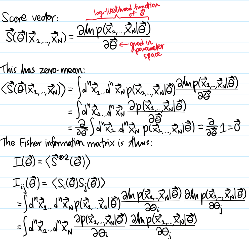
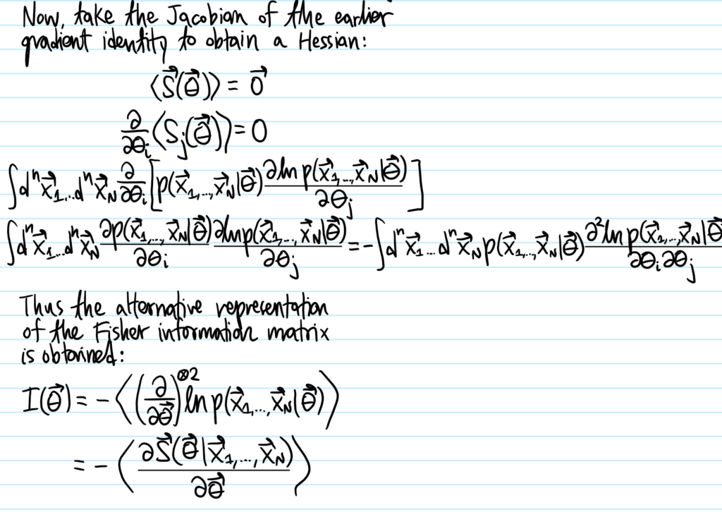
Problem: Define the score random vector \(\mathbf S(\boldsymbol{\theta})=\mathbf S(\boldsymbol{\theta}|\mathbf x_1,…,\mathbf x_N)\). Show that the covariance matrix of the score \(\mathbf S(\boldsymbol{\theta})\), called the Fisher information matrix \(I(\boldsymbol{\theta}):=\langle(\mathbf S(\boldsymbol{\theta})-\langle\mathbf S(\boldsymbol{\theta})\rangle)^{\otimes 2}\rangle\), may be written:
\[I(\boldsymbol{\theta})=-\biggr\langle\frac{\partial^2\ln p(\mathbf x_1,…,\mathbf x_N|\boldsymbol{\theta})}{\partial\boldsymbol{\theta}^2}\biggr\rangle\]
(all expectations \(\langle\space\rangle\) are of course over the joint distribution of the observed data \(\mathbf x_1,…,\mathbf x_N\) defined by the likelihood function \(p(\mathbf x_1,…,\mathbf x_N|\boldsymbol{\theta})\))
Solution:
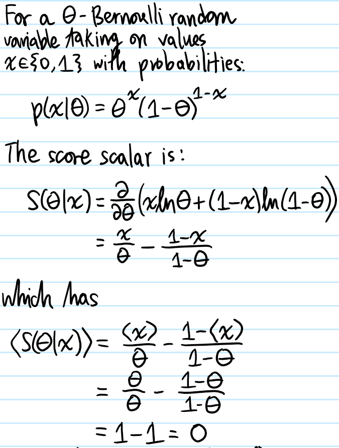
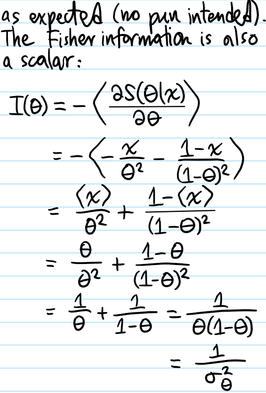
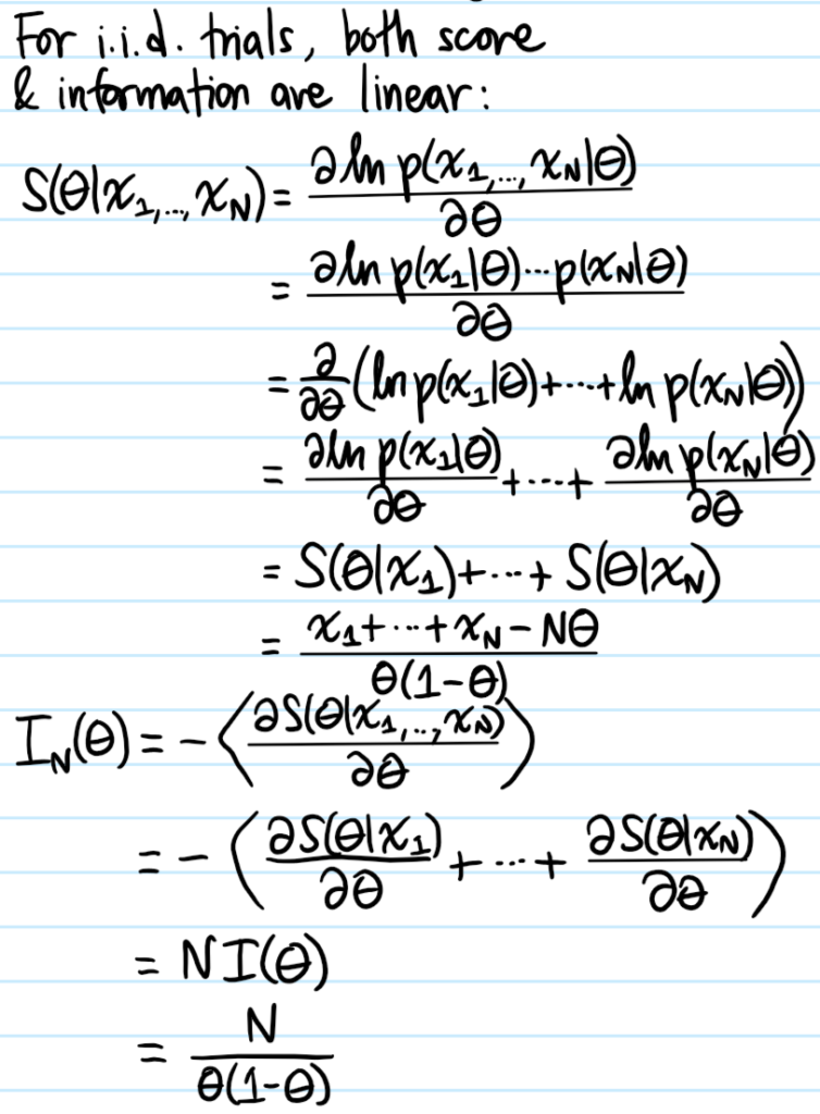
Problem: Calculate explicitly the score \(S(\theta|x)\) and Fisher information \(I(\theta)\) for a \(\theta\)-Bernoulli random variable with outcome \(x\in\{0,1\}\). Hence, what can be said about the score \(S(\theta|x_1,…,x_N)\) and Fisher information \(I_N(\theta)\) for the corresponding \(N\)-trial binomial random variable where each i.i.d. trial is \(\theta\)-Bernoulli?
Solution:
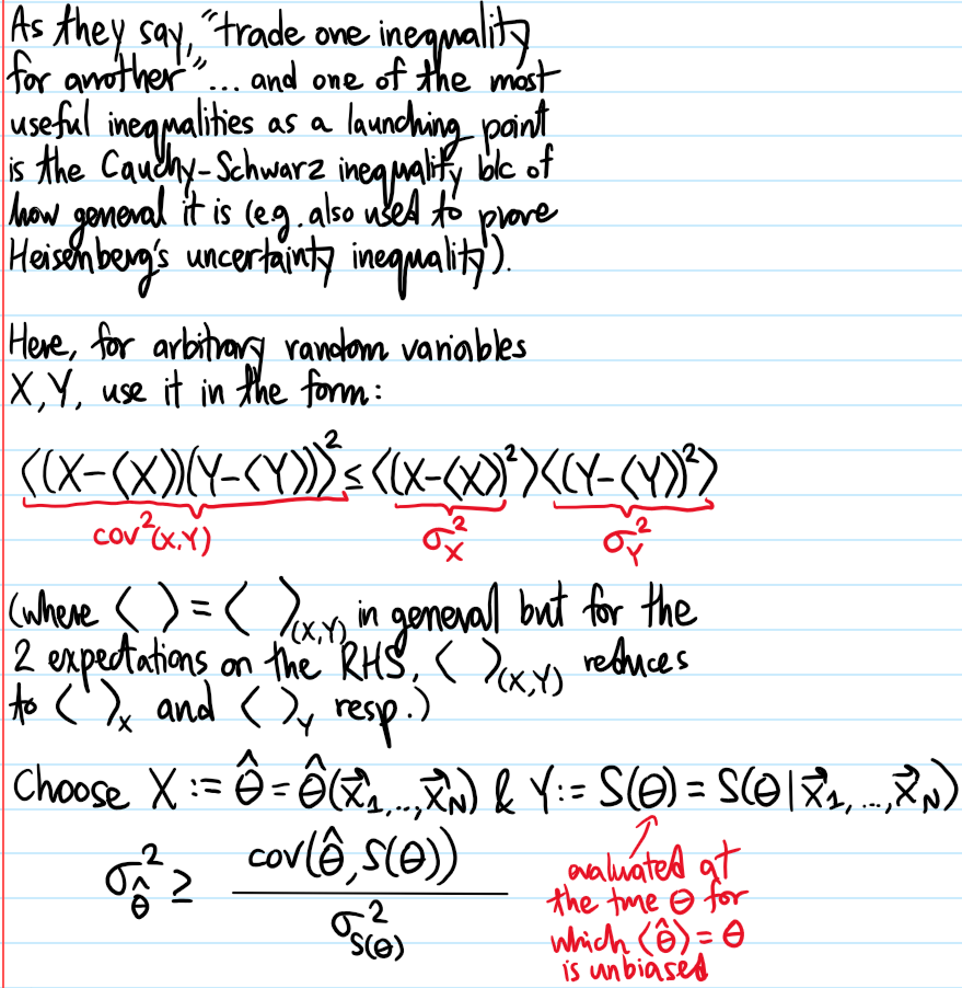
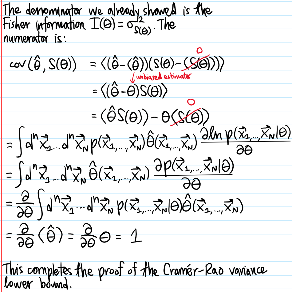
Problem: State and prove the Cramér-Rao variance lower bound.
Solution: Consider for simplicity attempting to estimate just a single, unknown, fixed scalar parameter \(\theta\) with an unbiased point estimator \(\hat{\theta}=\hat{\theta}(\mathbf x_1,…,\mathbf x_N)\). Then the Cramér-Rao variance lower bound asserts that the minimum possible variance of such an estimator \(\hat{\theta}\) is given by the inverse Fisher information evaluated at the true underlying value of the parameter \(\theta\) for which the point estimator \(\langle\hat{\theta}\rangle=\theta\) is unbiased:
\[\sigma^2_{\hat{\theta}}\geq\frac{1}{I(\theta)}\]
In the more general case where \(\langle\hat{\boldsymbol{\theta}}\rangle=\boldsymbol{\theta}\) is an unbiased point estimator for more than \(1\) parameter, a natural generalization holds:
\[\text{cov}(\hat{\boldsymbol{\theta}},\hat{\boldsymbol{\theta}})\geq I^{-1}(\boldsymbol{\theta})\]
where \(I^{-1}(\boldsymbol{\theta})\) is the inverse of the Fisher information matrix, and the meaning of this matrix inequality is that \(\text{cov}(\boldsymbol{\theta},\boldsymbol{\theta})-I^{-1}(\boldsymbol{\theta})\) is positive semi-definite.
Problem: Combining the results of the previous \(2\) problems, what can be deduced?
Solution: Naturally, one is interested in finding the minimum-variance unbiased estimator (MVUE) for some parameter. But the Cramér-Rao variance lower bound is precisely a statement about how low the variance can go. In particular, for the \((N,\theta)\)-binomial random variable, since \(\hat{\theta}=\sum_{i=1}^Nx_i/N\) was already shown to be an unbiased estimator for \(\theta\), and moreover its variance \(\sigma^2_{\hat{\theta}}=\theta(1-\theta)/N=1/I_N(\theta)\) saturates the Cramér-Rao variance lower bound, it must therefore be the MVUE for \(\theta\)!
Problem: How can random error be reduced in a scientific experiment? What about systematic error?
Solution: The standard error \(\sigma_{\hat{\mu}}=\sigma/\sqrt{N}\) can be taken as a quantitative proxy for the effective random error from \(N\) i.i.d. measurements. This reveals that there are \(2\) ways to reduce the effective random error:
- Reduce \(\sigma\) (e.g. cooling down electronics to mitigate Johnson noise).
- Increase \(N\) (make more measurements).
Reducing systematic error is a completely different beast, and requires techniques such as calibration against a “gold standard”, differential measurements, etc.
Problem: Explain how the \(\chi^2\) goodness-of-fit test arises from maximizing a log-likelihood function subject to normally distributed errors between the data and the model.
Solution: The \(\chi^2\) statistic is basically just a rearrangement of the usual formula for variance to isolate for \(N=\chi^2\). Indeed, comparing \(\chi^2\ll N,\chi^2\approx N,\chi^2\gg N\) basically is the whole point of the test. The subtraction of the number of constraints from \(N\) is also reminiscent of the Bessel correction, and in fact the \(2\) are there for conceptually the same reason.