
The purpose of this post is to contrast the classical treatment of Rutherford scattering with its quantum mechanical treatment. At the end, the surprise will be that for certain important quantities such as the differential cross-section, the classical and quantum scattering calculations agree with each other.
Classical Rutherford Scattering
Classically, Rutherford scattering refers to the scattering of classical particles by a repulsive Coulomb potential \(V(r)=\frac{k}{r}\) with \(k>0\) for a repulsive interaction. In the limit when the particle is far away, the eccentricity (Laplace-Runge-Lenz) vector \(\textbf e=\frac{\textbf p\times\textbf L}{mk}-\hat{\textbf x}\) approximately forms a right triangle as follows:
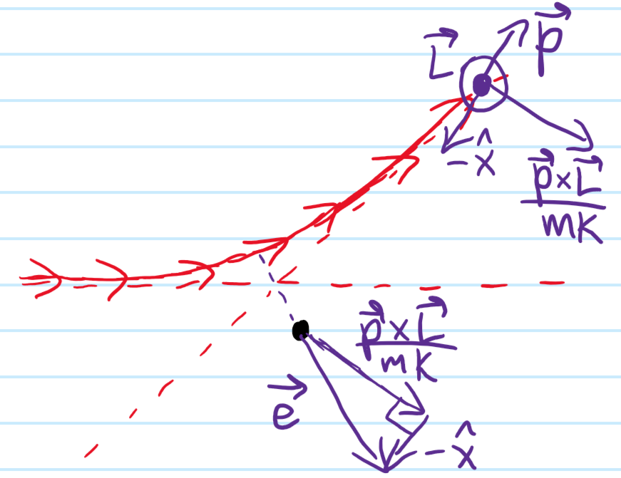
It follows from Pythagoras that \(e^2=1^2+\frac{p^2_{\infty}L^2}{m^2k^2}\) with \(L=\rho p_{\infty}\) proportional to the impact parameter \(\rho\). Thus, \(e^2=1+\frac{p^4_{\infty}\rho^2}{m^2k^2}\). We can then relate \(p_{\infty}^2=2mE\) with the mechanical energy \(E\) so that \(e^2=1+\left(\frac{2E\rho}{k}\right)^2\). Finally, the geometry of hyperbolas dictates that the scattering angle \(\theta\) is related to the eccentricity \(e\) by \(\cos\left(\frac{\pi}{2}-\frac{\theta}{2}\right)=\sin\left(\frac{\theta}{2}\right)=\frac{1}{e}\). Thus, one finds classically:
\[\tan\left(\frac{\theta}{2}\right)=\frac{|k|}{2E\rho}\]
More realistically, in scattering experiments one does not throw just one projectile at the scattering center, but rather fires a beam of projectiles. In light of this, recall that the classical differential cross-section \(d\sigma\) is defined to conserve particle number: \(\textbf J_{\text{incident}}\cdot d\boldsymbol{\sigma}=\textbf J_{\text{scattered}}\cdot d\textbf S\). If one imagines an infinitely thin and narrow cylindrical “washer” of \(N\) incident particles, then the incident particle density is \(n=\frac{N}{2\pi\rho d\rho dz}\). Supposing moreover the incident particles move at velocity \(v\), then \(J_{\text{incident}}=nv=\frac{Nv}{2\pi\rho d\rho dz}\). On the other hand by energy conservation \(\dot E=0\) the scattered particles eventually are moving at the same velocity \(v\). The scattering current is therefore \(J_{\text{scattered}}=\frac{Nv}{2\pi r\sin\theta rd\theta dz}\). Finally, using \(dS=r^2 d\Omega\) and isolating for the differential cross-section gives:
\[d\sigma=\rho\csc\theta\left|\frac{\partial\rho}{\partial\theta}\right|d\Omega\]
For the case of Rutherford scattering from a Coulomb potential, the differential cross-section is:
\[d\sigma=\left(\frac{k}{4E}\right)^2\csc^4\frac{\theta}{2}d\Omega\]
The total cross section is:
\[\sigma=\int d\sigma=2\pi\left(\frac{k}{4E}\right)^2\int_{0}^{\pi}\csc^4\frac{\theta}{2}\sin\theta d\theta\]
However, it turns out that the integrand has an antiderivative \(-2\csc^2\left(\frac{\theta}{2}\right)\) which blows up to \(\infty\) at \(\theta=0\) so that the total cross section \(\sigma=\infty\)! It turns out this has to do with the fact that, although the Coulomb potential \(V(r)=\frac{k}{r}\) decays to \(V(r)\to 0\) as \(r\to\infty\), it does so “too slowly” so that it’s ultimately a long-range force and so all incident particles feel its repulsive scattering influence “to some non-zero extent” so that \(\sigma=\infty\).
Quantum Rutherford Scattering
Although the result for the differential cross-section \(d\sigma\) for Rutherford scattering was obtained through classical mechanics alone, it turns out to agree with quantum mechanical scattering calculations. To demonstrate this, it is helpful to first take a step back and analyze a generic central potential \(V(r)\) which (both classically and quantum mechanically) conserves total angular momentum. Recall in this case, the Schrodinger equation is a separable linear PDE in spherical coordinates with solutions of the form \(\psi(r,\theta,\phi)=\sum_{\ell=0}^{\infty}\sum_{m=-\ell}^{\ell}R_{\ell}(r)Y_{\ell}^{m}(\theta,\phi)\). However, by scattering incident particles along the \(z\)-axis, in our case we expect not just asymptotically but everywhere that \(\partial\psi/\partial\phi=0\Rightarrow L_3\psi=0\) has angular momentum confined to the \(xy\)-plane and so one can set \(m=0\) to reduce the spherical harmonics \(Y_{\ell}^0\propto P_{\ell}(\cos\theta)\) to Legendre polynomials. Redefining the radial functions to absorb any constants, the spherical harmonic expansion of \(\psi(r,\theta,\phi)\) earlier therefore reduces to a partial wave expansion of \(\psi(r,\theta)\):
\[\psi(r,\theta)=\sum_{\ell=0}^{\infty}R_{\ell}(r)P_{\ell}(\cos\theta)\]
specifically, the original linear Schrodinger PDE can be thought of as separating into a linear ODE \(\textbf L^2P_{\ell}(\cos\theta)=\ell(\ell+1)\hbar^2P_{\ell}(\cos\theta)\) that defines the Legendre polynomials and a linear ODE for the radial amplitude \(R_{\ell}(r)\) which depends on the exact nature of the central potential \(V(r)\):
\[\frac{d^2R_{\ell}}{dr^2}+\frac{2}{r}\frac{dR_{\ell}}{dr}-\left(\frac{\ell(\ell+1)}{r^2}+\frac{2m}{\hbar^2}(V(r)-E)\right)R_{\ell}(r)=0\]
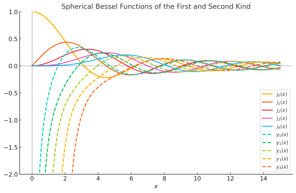
First, suppose \(V(r)=0\) everywhere so that there isn’t really any scattering going on (i.e. the Schrodinger equation reduces to a Helmholtz equation). Then as is well-known the radial amplitude \(R_{\ell}(r)\) is given by linear combinations of spherical Bessel functions \(j_{\ell}(kr),y_{\ell}(kr)\) where \(k:=\sqrt{2mE}/\hbar\) and we have the Rodrigues-type formulas for the spherical Bessel functions (sometimes called Rayleigh’s formulas):
\[j_{\ell}(x)=(-x)^{\ell}\left(\frac{1}{x}\frac{d}{dx}\right)^{\ell}\text{sinc}(x)\]
\[y_{\ell}(x)=-(-x)^{\ell}\left(\frac{1}{x}\frac{d}{dx}\right)^{\ell}\text{cosc}(x)\]
where \(\text{cosc}(x):=\cos(x)/x\) makes the spherical Bessel function \(y_{\ell}(x)\) singular at the origin \(x=0\) (the minus sign in front of \(y_{\ell}(x)\) is also merely conventional). It is common to treat the spherical Bessel functions as real and imaginary parts of complex-valued spherical Hankel functions \(h_{\ell}^{(1)}(x):=j_{\ell}(x)+iy_{\ell}(x)\) and \(h_{\ell}^{(2)}(x):=\overline{h_{\ell}^{(1)}(x)}=j_{\ell}(x)-iy_{\ell}(x)\). An especially important case are the \(\ell=0\) \(s\)-waves \(j_0(x)=\text{sinc}(x)\) and \(y_0(x)=-\text{cosc}(x)\), in which case \(h_0^{(1)}(x)=\frac{e^{-ix}}{x}\) and \(h_0^{(2)}(x)=\frac{e^{ix}}{x}\).
For example, the incident plane wave \(\psi(r,\theta)=e^{ikz}=e^{ikr\cos\theta}\) by itself is clearly a solution of the free Schrodinger equation. By linearity, it must therefore be possible to write such a plane wave \(e^{ikz}\) in terms of free partial waves of the form \((\alpha_{\ell}j_{\ell}(kr)+\beta_{\ell}y_{\ell}(kr))P_{\ell}(\cos\theta)\) for \(\ell\in\textbf N\). Indeed, because \(e^{ikz}\) is non-singular anywhere, we only require the spherical Bessel functions \(j_{\ell}(kr)\) of the first kind so \(\beta_{\ell}=0\). The expansion turns out to be (use orthogonality of Legendre polynomials):
\[e^{ikz}=e^{ikr\cos\theta}=\sum_{\ell=0}^{\infty}(2\ell+1)i^{\ell}j_{\ell}(kr)P_{\ell}(\cos\theta)\]
Close to the origin \(x\to 0\), the spherical Bessel functions behave like (for \(j_{\ell}(x)\) this is just saying that its Taylor series has its first non-zero term at order \(x^{\ell}\) so that \(d^{\ell}j_{\ell}/dx^{\ell}(x=0)=\ell!/(2\ell+1)!!\); for \(y_{\ell}(x)\) it diverges at \(x=0\) hence being non-differentiable there):
\[j_{\ell}(x)\to\frac{x^{\ell}}{(2\ell+1)!!}\]
\[y_{\ell}(x)\to -\frac{(2\ell-1)!!}{x^{\ell+1}}\]
where for example the double factorial \(!!\) is defined (not as the double application of the usual factorial, but rather) by \(5!!=5\times 3\times 1=15\). Asymptotically \(x\to\infty\), the spherical Bessel functions decay like:
\[j_{\ell}(x)\to\frac{\sin(x-\ell\pi/2)}{x}\]
\[y_{\ell}(x)\to-\frac{\cos(x-\ell\pi/2)}{x}\]
If you stare at the graphs above, these properties all seem pretty reasonable. In particular, when the asymptotic \(r\to\infty\) behavior is applied to the plane wave \(\psi(r,\theta)=e^{ikz}=e^{ikr\cos\theta}\), this becomes:
\[e^{ikz}\to\frac{1}{2ikr}\sum_{\ell=0}^{\infty}(2\ell+1)(e^{ikr}-(-1)^{\ell}e^{-ikr})P_{\ell}(\cos\theta)\]
Finally, as in one-dimensional scattering, in the steady state we want the asymptotic wavefunction \(\psi_{\infty}(r,\theta)\) to be not just an incident plane wave \(e^{ikz}=e^{ikr\cos\theta}\) of energy \(E=\hbar^2k^2/2m\) but also to comprise a scattered spherical wave (of the same energy \(E\)) which we therefore write as \(f(\theta)e^{ikr}/r\) for a complex-valued scattering amplitude \(f(\theta)\in\textbf C\) (dependent on the nature of the potential \(V(r)\) one is scattering off of and the incident momentum \(k\) of the beam) modulating the spherical Hankel \(s\)-wave \(e^{ikr}/r\):
\[\psi_{\infty}(r,\theta)=e^{ikz}+f(\theta)\frac{e^{ikr}}{r}\]
This ansatz certainly solves the Schrodinger equation asymptotically \(r\to\infty\) because asymptotically we expect \(V(r)\to 0\) which reduces to the earlier analysis where we had pretended \(V(r)=0\) everywhere. If we could compute the scattering amplitude \(f(\theta)\), then we immediately obtain the differential cross-section because \(J_{\text{incident}}=\frac{\hbar k}{m}\), \(J_{\text{scattered}}=\frac{\hbar k}{mr^2}|f(\theta)|^2\) so we have the fundamental relation \(d\sigma=|f(\theta)|^2d\Omega\) and as a corollary the cross-section itself is \(\sigma=2\pi\int_{-1}^{1}|f(\theta)|^2d\cos\theta\) (however, it turns out this corollary can be strengthened to the optical theorem \(\sigma=\frac{4\pi}{k}\Im f(0)\) where all the information about the potential \(V(r)\) is contained in the forward scattering amplitude \(f(0)\)).
Now, by expanding the scattering amplitude itself in a simplified partial wave basis \(f(\theta)=\sum_{\ell=0}^{\infty}f_{\ell}P_{\ell}(\cos\theta)\), this leads to the partial wave expansion of the asymptotic wavefunction:
\[\psi_{\infty}(r,\theta)=\frac{1}{2ik}\sum_{\ell=0}^{\infty}(2\ell+1)\left[\left(1+\frac{2ikf_{\ell}}{2\ell+1}\right)\frac{e^{ikr}}{r}+(-1)^{\ell+1}\frac{e^{-ikr}}{r}\right]P_{\ell}(\cos\theta)\]
From this, we conclude that there are countably infinitely many \(U(1)\) eigenvalues of the scattering \(S\)-operator, one for each \(\ell\in\textbf N\) given by \(e^{2i\delta_{\ell}(k)}=1+\frac{2ikf_{\ell}}{2\ell+1}\) (remember that the \(f_{\ell}\in\textbf C\)). In particular, the optical theorem then follows from orthogonality of the Legendre polynomials:
\[\sigma=2\pi\sum_{\ell=0}^{\infty}\sum_{\ell’=0}^{\infty}f_{\ell}f^*_{\ell’}\int_{-1}^1 P_{\ell}(\cos\theta)P_{\ell’}(\cos\theta)d\cos\theta=4\pi\sum_{\ell=0}^{\infty}\frac{|f_{\ell}|^2}{2\ell+1}\]
One can then isolate \(f_{\ell}=(e^{2i\delta_{\ell}(k)}-1)(2\ell+1)/2ik\) and substitute into the above, and compare with \(f(0)=\sum_{\ell=0}^{\infty}f_{\ell}\) to check the optical theorem’s validity. Furthermore, writing \(\sigma=\sum_{\ell=0}^{\infty}\sigma_{\ell}\) with each contribution cross-section \(\sigma_{\ell}=\frac{4\pi(2\ell+1)\sin^2\delta_{\ell}(k)}{k^2}\leq\frac{4\pi(2\ell+1)}{k^2}\) is called a unitarity bound (since it arises from the unitarity of the \(S\)-operator). This unitarity bound can be understood semiclassically (not entirely classical because it does use quantum mechanics), by imagining a beam of classical particles all incident on the scattering center with momentum \(k\). Then, look at some particle with impact parameter \(\rho\) and hence angular momentum \(L=\hbar k\rho\). This should be quantized as \(L=\ell\hbar\), so suppose that \(\rho\in[\ell/k,(\ell+1)/k]\) corresponds to a given quantization. Then in the ideal case when the particle is \(100\%\) scattered, this idealized area \(\sigma_{\ell}^*\) of the annulus into which it scatters:
\[\sigma_{\ell}^*=\pi\left(\frac{\ell+1}{k}\right)^2-\pi\left(\frac{\ell}{k}\right)^2=\frac{\pi(2\ell+1)}{k^2}\]
which is the unitary bound \(\sigma_{\ell}\leq 4\sigma_{\ell}^*\) up to the factor of \(4\).
Scattering Off Hard Spheres
Although we’d ultimately like to understand Rutherford scattering quantum mechanically, it helps to first look at a few simpler examples. The first is the infinitely hard sphere of radius \(a\), defined by \(V(r)=\infty\) for \(r<a\) and \(V(r)=0\) for \(r>a\). Basically, outside the hard sphere we have the usual solution \(\psi(r,\theta)=\sum_{\ell=0}^{\infty}(\alpha_{\ell}j_{\ell}(kr)+\beta_{\ell}y_{\ell}(kr))P_{\ell}(\cos\theta)\) whereas inside the hard sphere the wavefunction \(\psi(r<a)=0\) vanishes. First, we need to remember that we’re scattering off this sphere. This means that, asymptotically, the wavefunction \(\psi(r,\theta)\) needs to look like \(\psi_{\infty}(r,\theta)=\frac{1}{2ik}\sum_{\ell=0}^{\infty}(2\ell+1)\left[e^{2i\delta_{\ell}(k)}\frac{e^{ikr}}{r}+(-1)^{\ell+1}\frac{e^{-ikr}}{r}\right]P_{\ell}(\cos\theta)\). Using the asymptotic \(r\to\infty\) expansions of the spherical Bessel functions given earlier, one can check that \(e^{2i\delta_{\ell}(k)}=\frac{\alpha_{\ell}-i\beta_{\ell}}{\alpha_{\ell}+i\beta_{\ell}}\) which implies that the ratio of the probability amplitudes \(\beta_{\ell}/\alpha_{\ell}\) is simply (note that only this ratio is physically significant, not their absolute values because scattering states are not normalized anyways):
\[\frac{\beta_{\ell}}{\alpha_{\ell}}=-\tan\delta_{\ell}(k)\]
Finally, the Dirichlet boundary condition \(\psi(a)=0\) implies that \(\alpha_{\ell}j_{\ell}(ka)+\beta_{\ell}y_{\ell}(ka)=0\) for all \(\ell\in\textbf N\) so that the scattering phase shifts \(\delta_{\ell}(k)\in\textbf R\) are given simply by:
\[\tan\delta_{\ell}(k)=\frac{j_{\ell}(ka)}{y_{\ell}(ka)}\]
For instance, \(\delta_0(k)=-ka\) is exactly a linear phase shift for this specific case of scattering off a hard sphere. The higher-\(\ell\) phase shifts \(\delta_{\ell}(k)\) wrap like so:
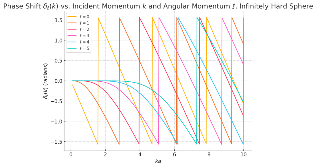
We are now in a position to compute the cross-section \(\sigma=\frac{4\pi}{k^2}\sum_{\ell=0}^{\infty}(2\ell+1)\sin^2\delta_{\ell}(k)\). First, consider just the low-momentum \(ka\ll 1\) limit whereby, applying the near-origin behavior of the spherical Bessel functions, we obtain the corresponding low-momentum behavior of the phase shifts \(\delta_{\ell}(k)\approx -\frac{(ka)^{2\ell+1}}{(2\ell+1)!!(2\ell-1)!!}\) (this qualitatively agrees with the graphs above). The infinite series for the cross-section \(\sigma_{ka\ll 1}\) in this low-momentum limit \(ka\ll 1\) is therefore:
\[\sigma_{ka\ll 1}=\frac{4\pi}{k^2}\sum_{\ell=0}^{\infty}(2\ell+1)\sin^2\left(-\frac{(ka)^{2\ell+1}}{(2\ell+1)!!(2\ell-1)!!}\right)\]
But since each \(\delta_{\ell}(k)\) is a monomial in \(ka\) but we’re working in the low-momentum limit \(ka\ll 1\) so each \(\delta_{\ell}(k)\) is almost zero (again, see the graph too), allowing us to apply a small-angle approximation \(\sin^2\left(-\frac{(ka)^{2\ell+1}}{(2\ell+1)!!(2\ell-1)!!}\right)\approx\frac{(ka)^{4\ell+2}}{(2\ell+1)!!^2(2\ell-1)!!^2}\):
\[\sigma_{ka\ll 1}\approx \frac{4\pi}{k^2}\sum_{\ell=0}^{\infty}(2\ell+1)\frac{(ka)^{4\ell+2}}{(2\ell+1)!!^2(2\ell-1)!!^2}\]
Finally, we see that for \(\ell\geq 1\gg ka\) the monomials \((ka)^{4\ell+2}\) go to zero especially rapidly as \(\ell\to\infty\). The only phase shift that goes to zero but not as rapidly as the others is the \(\ell=0\) \(s\)-wave phase shift \(\delta_0(k)=-ka\) (again, all this is apparent from the graph). Thus, keeping only the dominant \(\ell=0\) term in the series gives finally:
\[\sigma_{ka\ll 1}\approx \frac{4\pi}{k^2}(-ka)^2=4\pi a^2\]
which is \(4\times\) greater than the classical geometric cross-section \(\sigma_{\text{classical}}=\pi a^2\) for scattering billiard balls off the hard sphere (i.e. it is now the surface area of the hard sphere rather than its cross-sectional area, so still using the name “cross-section” for \(\sigma\) is strictly a misnomer).
Although above we reasoned all the approximations made in the calculation of the low-energy scattering cross-section \(\sigma_{ka\ll 1}\) purely mathematically (e.g. monomials, etc.), there is a nice semiclassical “physics way” to understand it too. Just as earlier with the semiclassical argument for the unitarity bound, imagine scattering classical particles with impact parameter \(\rho:=\ell/k\) in which case the regime \(\ell\gg ka\) (such as \(\ell\geq 1\gg ka\) above) is merely the regime \(\rho\gg a\) where the classical particle flies in far away from the scattering center \(r=0\), so it makes sense that it’s not really going to be scattered much/feel the influence of \(V(r)\), hence the phase shift \(\delta_{\ell}(k)\approx 0\) is negligible for \(\ell\geq 1\). Instead, only when you throw the particles head-on at the scattering center, which corresponds to the \(\ell=0\) \(s\)-wave do they accumulate a “somewhat noticeable” phase shift \(\delta_0(k)=-ka\) when \(ka\ll 1\).
Finally, just briefly, let’s also look at the high-momentum \(ka\gg 1\) regime. Here, applying far-field asymptotics of the spherical Bessel functions, all the phase shifts become lines displaced vertically in units of \(90^{\circ}=\pi/2\) from each other \(\delta_{\ell}(k)\approx -ka+\ell\pi/2\) (graph agrees with this). In this high-momentum \(ka\gg 1\) limit, the cross-section \(\sigma_{ka\gg 1}\) is:
\[\sigma_{ka\gg 1}=\frac{2\pi a^2}{(ka)^2}\sum_{\ell=0}^{\infty}(2\ell+1)(1-(-1)^{\ell}\cos 2ka)\]
which tends to \(\sigma\to 2\pi a^2\) as one lets \(ka\to\infty\) (hemispherical surface area?).
Universal Dynamics of Low-Energy Scattering
Okay, now let’s go back to low-energy (equivalently low-momentum) scattering. We already saw for the hard sphere that for each quantized angular momentum \(\ell\in\textbf N\), the phase shift \(\delta_{\ell}(k)\) scaling law at low-momentum \(ka\ll 1\) was:
\[\delta_{\ell}(k)\propto -(ka)^{2\ell+1}\]
It turns out, if we replace the hard sphere radius \(a\mapsto a_s\) by a more general characteristic scattering length \(a_s\) unique to each potential \(V(r)\) (e.g. \(a_s=a\) for the hard sphere potential), then this power law scaling is a universal phenomenon; in any scattering central potential \(V(r)\), when one throws quantum particles at it slowly \(ka_s\ll 1\) with some angular momentum \(\ell\) misaligned from the scattering center, the phase shift \(\delta_{\ell}(k)\propto -(ka_s)^{2\ell+1}\) decays as an odd power of \(ka_s\). And as before, really the only noticeable phase shift is associated with the head-on \(\ell=0\) \(s\)-wave with \(\delta_0(k)=-ka_s+O_{ka_s\ll 1}(ka_s)^3\). By repeating verbatim the approximation used in calculating \(\sigma_{ka\ll 1}\), one can check that we also have a characteristic low-energy cross-section \(\sigma_{ka_s\ll 1}=4\pi a_s^2\) the surface area of a fictitious sphere \(S^2_{a_s}\) of radius equal to the potential’s scattering length \(a_s\).
Why Bound/Resonant States Cause \(a_s\to\pm\infty\) to Diverge
If an attractive central potential \(V(r)\) with \(dV/dr>0\) (so not the hard sphere potential which was repulsive \(dV/dr<0\)) happens to be sufficiently attracting that it admits the possibility of trapping a quantum particle inside a bound or resonant state, then the mere existence (or “almost-existence”) of such a bound/resonant state will strongly affect scattering states (it’s like kicking a soccer ball into a valley, if the valley is deep enough then it will interact significantly with the soccer ball to slow it down and attempt to trap it). More precisely, one of the most pronounced such effects is that the potential’s scattering length \(a_s\to\pm\infty\) will diverge to infinity whenever there is a threshold bound or resonant state (intuitively, this says when you throw the particle slowly and head-on at \(V(r)\), the particle looks like it scatters off a hard sphere of radius \(a_s\), except that \(a_s>0\) means it’s repelled whereas \(a_s<0\) means it’s attracted while \(a_s=0\) means no scattering).
The simplest model system in which to see this phenomenon of divergence is the finite spherical potential well of radius \(a\) and depth \(V_0>0\). We already know that when \(V_0\) is deep enough or \(a\) is big enough, bound states should start to appear. First, we know outside \(r>a\) we have the same solution as the hard sphere \(\psi(r,\theta)=\sum_{\ell=0}^{\infty}(\alpha_{\ell}j_{\ell}(kr)+\beta_{\ell}y_{\ell}(kr))P_{\ell}(\cos\theta)\). Since we’re still matching this to the same “asymptotic boundary condition” \(\psi_{\infty}(r,\theta)=\frac{1}{2ik}\sum_{\ell=0}^{\infty}(2\ell+1)\left[e^{2i\delta_{\ell}(k)}\frac{e^{ikr}}{r}+(-1)^{\ell+1}\frac{e^{-ikr}}{r}\right]P_{\ell}(\cos\theta)\), this still leads to the same condition on the phase shifts:
\[\tan\delta_{\ell}=-\frac{\beta_{\ell}}{\alpha_{\ell}}\]
The difference now though is that inside the finite spherical potential well the wavefunction is \(\psi(r,\theta)=\sum_{\ell=0}^{\infty}\gamma_{\ell}j_{\ell}(k’r)P_{\ell}(\cos\theta)\) with \(k’^2=k^2+2mV_0/\hbar^2\) with no second-kind spherical Bessel functions \(y_{\ell}(k’r)\) due to the requirement of regularity at the origin \(r=0\). By matching the logarithmic derivative of \(\psi(r,\theta)\) at \(r=a\) to eliminate the unwanted \(\gamma_{\ell}\) unknowns, calculating derivatives of spherical Bessel functions by just directly applying the product rule on their Rayleigh-definitions, and doing some algebra gets:
\[\tan\delta_{\ell}(k)=\frac{kaj_{\ell+1}(ka)j_{\ell}(k’a)-k’aj_{\ell}(ka)j_{\ell+1}(k’a)}{kaj_{\ell}(k’a)y_{\ell+1}(ka)-k’aj_{\ell+1}(k’a)y_{\ell}(ka)+\ell j_{\ell}(k’a)[y_{\ell}(ka)-y_{\ell+1}(ka)]}\]
In particular, for \(\ell=0\) \(s\)-wave scattering:
\[\tan\delta_0(k)=\frac{k\cos ka\sin k’a-k’\cos k’a\sin ka}{k\sin ka\sin k’a+k’\cos ka\cos k’a}\]
So far everything has been exact. Now come the approximations. The first is the usual low-energy scattering limit \(ka\ll 1\), the second is that \(k\ll \sqrt{2mV_0}/\hbar\), or equivalently we can assume \(k’\approx\sqrt{2mV_0}/\hbar\) is approximately independent of \(k\) in what follows. Artificially multiplying numerator and denominator by \(a\) allows one to write:
\[\tan\delta_0(k)=\frac{x\cos x\sin k’a-k’a\cos k’a\sin x}{x\sin x\sin k’a+k’a\cos x\cos k’a}\]
with \(x:=ka\) the parameter we’re taking to be \(x\ll 1\). After a calculation, one can check that the right-hand side, Taylor expanded about \(x=0\) to first-order yields:
\[\tan\delta_0(k)\approx(\text{tanc}(k’a)-1)x\]
Finally, assuming that even for this \(\ell=0\) \(s\)-wave the phase shift \(\delta_{\ell}(k)\) is sufficiently small so that \(\tan\delta_0(k)\approx\delta_0(k)\):
\[\delta_0(k)\approx(\text{tanc}(k’a)-1)ka\]
allows us to directly read off the scattering length as:
\[a_s=a(1-\text{tanc}(k’a))\]
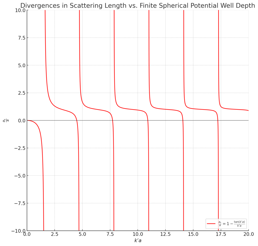
By virtue of the tangent function, the scattering length \(a_s\) of the finite spherical potential well diverges at \(k’a=\pi(n+1/2)\), corresponding (in our approximation scheme) to potential well depths of the form \(V_0=\frac{(n+1/2)^2\pi^2\hbar^2}{2ma^2}\). Note that we’re implicitly assuming it’s a potential well \(V_0>0\); if it had been a finitely hard sphere \(V_0<0\) instead, then we would have an imaginary momentum \(k’=\sqrt{2mV_0}/\hbar=i\sqrt{-2mV_0}/\hbar\) and using \(\tan i\theta=i\tanh\theta\), we would conclude that instead the scattering length \(a_s\) is given by:
\[a_s=a\left[1-\text{tanhc}\left(\frac{\sqrt{-2mV_0}a}{\hbar}\right)\right]\]
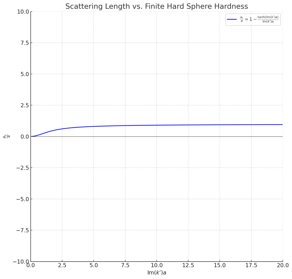
in which there is no longer any trace of the divergences \(a_s=\pm\infty\) seen earlier with the attractive well \(V_0>0\) (but rather, as the graph shows, when the sphere gets infinitely hard \(\Im(k’)a\to\infty\), the scattering length \(a_s\to a\) converges back to our earlier result of the hard sphere radius \(a\)). This hints that the divergences have something to do with the potential being attractive \(V_0>0\) and from its quantized nature and the formula for the depths \(V_0\), it’s natural to conjecture that it has something to do with bound/resonant states coming into existence associated with said attractive potential. This connection can be clarified by looking for imaginary momenta \(k=-i\kappa\) on the lower imaginary axis \(\kappa\in(0,\infty)\) such that the \(S\)-operator eigenvalue \(e^{2i\delta_{0}(k)}=0\) associated to the \(\ell=0\) \(s\)-wave vanishes. But we already found earlier while matching asymptotic boundary conditions that we have exactly:
\[e^{2i\delta_0(k)}=\frac{\alpha_0-i\beta_0}{\alpha_0+i\beta_0}=\frac{1+i\tan\delta_0(k)}{1-i\tan\delta_0(k)}\]
which is simply the trivially obvious identity \(e^{2i\theta}=(1+i\tan\theta)/(1-i\tan\theta)\). This vanishes whenever the numerator \(\tan\delta_0(k)=i\) vanishes. Now, working with the exact formula for \(\tan\delta_0(k)\) from earlier (i.e. not touching any of the approximate formulas!) one finds that this implies:
\[\tan k’a=-\frac{k’}{\kappa}\]
where any value of \(\kappa\in (0,\infty)\) we can find that solves this equation (keeping in mind \(k’\) is defined in terms of \(\kappa\) via \(k’^2=-\kappa^2+2mV_0/\hbar^2\)) implies a bound state with energy \(E=-\hbar^2\kappa^2/2m<0\). Exactly at \(k=\kappa=E=0\) however so that \(k’=\sqrt{2mV_0}/\hbar\), one obtains a bound state at threshold whenever \(k’a=\pi (n+1/2)\) which reproduces the potential well depths \(V_0=\frac{(n+1/2)^2\pi^2\hbar^2}{2ma^2}\) at which the scattering length \(a_s\) diverges. Moreover, for a general zero of \(e^{2i\delta_0(k)}\) at some \(k=-i\kappa\), if one Laurent-expands \(e^{2i\delta_0(k)}=\frac{1+i\tan\delta_0(k)}{1-i\tan\delta_0(k)}\) about \(k=-i\kappa\), then because \(e^{2i\delta_0(k)}\in U(1)\) it must look like a Mobius transformation \(e^{2i\delta_0(k)}\approx\frac{k+i\kappa}{k-i\kappa}\) for \(k\) near \(-i\kappa\) so in other words \(\tan\delta_0(k)\approx -k/\kappa\). Approximating \(\tan\delta_0(k)\approx\delta_0(k)\) then yields \(a_s=1/\kappa\) which indeed diverges as \(\kappa\to 0\).
Breit-Wigner Distribution
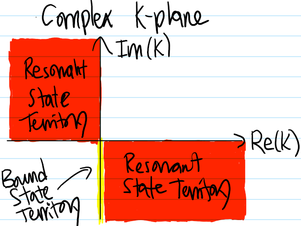
Recall that while “scattering states” with lower imaginary momenta \(k=-i\kappa\) that suppress the scattering \(e^{2i\delta_0(k)}=0\) are actually bound states with energy \(E=-\hbar^2\kappa^2/2m\) in disguise, we also saw that “scattering states” with complex momenta in quadrant \(2\) or \(4\) of the complex \(k\)-plane \(\Re k\Im k<0\) that suppress the scattering \(e^{2i\delta_0(k)}=0\) are actually resonant states with complex energy \(E = \frac{\hbar^2 (\Re^2 k – \Im^2 k)}{2m} + i \frac{\hbar^2}{m} \Re k\Im k\) in disguise with lifetime \(\tau=-m/\hbar\Re k\Im k>0\) and energy width \(\Gamma/2=\hbar/\tau\).
This allows us to write the resonant state’s complex energy in the form \(E=E_{\text{CoM}}-i\Gamma/2\) where the center of mass energy is \(E_{\text{CoM}}:=\Re E=\frac{\hbar^2 (\Re^2 k – \Im^2 k)}{2m}\). Viewing the complex momentum \(k=\sqrt{2mE}/\hbar\) as a function of the complex energy \(E\), we can thus also view the \(U(1)\) phase \(e^{2i\delta_{\ell}(k)}=e^{2i\delta_{\ell}(E)}\) as a function of \(E\) rather than \(k\). Specifically, if \(e^{2i\delta_0(E=E_0-i\Gamma/2)}=0\), then in a neighbourhood of this complex energy \(E=E_{\text{CoM}}-i\Gamma/2\), the map \(E\mapsto e^{2i\delta_0(E)}\) looks locally like a Mobius transformation:
\[e^{2i\delta_{\ell}(E)}\approx \frac{E-E_{\text{CoM}}+i\Gamma/2}{E-E_{\text{CoM}}-i\Gamma/2}\]
up to a \(U(1)\) continuum contribution that we don’t care about. This can be algebraically rearranged to yield a Lorentzian distribution:
\[\sin^2\delta_{\ell}(E)=\frac{\Gamma^2}{4(E-E_{\text{CoM}})^2+\Gamma^2}\]
which directly yields the scattering cross-section \(\sigma_{\ell}(E)\) as a function of the complex energy \(E\) for partial waves of angular momentum \(\ell\):
\[\sigma_{\ell}(E)=\frac{2\pi\hbar^2}{mE}(2\ell+1)\frac{\Gamma^2}{4(E-E_{\text{CoM}})^2+\Gamma^2}\]
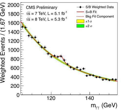
This is (roughly speaking) known in particle physics as the Breit-Wigner distribution for the cross-section. If we artificially restrict to \(E\in\textbf R\), then one can plot \(\sigma_{\ell}(E)\) and it looks pretty much like \(1/E\) modulated by a Lorentzian “bell curve”, sort of like the discovery of the Higgs boson:
The Breit-Wigner distribution maximizes \(d\sigma_{\ell}/dE=0\) at \(E=\frac{2}{3}E_{\text{CoM}}+\frac{1}{3}\sqrt{E_{\text{CoM}}^2-\frac{3}{4}\Gamma^2}\), though it’s basically always the case that the center of mass energy \(E_{\text{CoM}}\gg\Gamma\) is much greater than the energy width \(\Gamma\) of the particle’s resonant state so that we can basically just focus on maximizing the Lorentzian piece \(\frac{\Gamma^2}{4(E-E_{\text{CoM}})^2+\Gamma^2}\) which is trivially maximized to \(1\) at its center when the denominator is minimized at \(E=E_{\text{CoM}}\) and agrees with the above quadratic formula result. The corresponding maximal cross-section (typically measured in units of \(1\text{ barn}=10^{-28}\text{ m}^2\) in experiment) is therefore \(\sigma_{\ell}^*\approx\frac{2\pi\hbar^2}{mE_{\text{CoM}}}(2\ell+1)=2\pi\bar{\lambda}^2(2\ell+1)\) where \(\bar{\lambda}:=\hbar/mc\) is the reduced Compton wavelength of the particle by virtue of \(E_{\text{CoM}}=mc^2\) which saturates the unitarity bound. Finally, although the Lorentzian distribution is one of those pathological probability distributions with undefined mean (and by extension, undefined variance, and all higher-order moments), it still has a perfectly well-defined \(\text{FWHM}=\Gamma\) hence explaining why \(\Gamma\) has been called the energy width the whole time.
A particle accelerator’s job is to basically vary the incident energy \(E\) and measure the corresponding cross-section \(\sigma(E)\). It is a fundamental fact of nature that most particles are very unstable with short lifetimes \(\tau\). The stable exceptions are protons \(p^+\), electrons \(e^-\), photons \(\gamma\), neutrinos \(\nu\), etc. By colliding these stable particles, unstable ones can emerge briefly in such collisions, but only appear as resonant states which quickly decay with short lifetime \(\tau\).
Lippman-Schwinger Equation, Born Series Approximation
Suppose we write the Hamiltonian for a scattering process perturbatively as \(H=\tilde H+\Delta\tilde H\), where \(\tilde H\) is some well-understood Hamiltonian and \(\Delta\tilde H\) is a small perturbation to it. Most often, we’ll take \(\tilde H=T\) to just be the kinetic energy operator and \(\Delta\tilde H:=V\) to be the potential energy from which one is scattering (this is the same view taken in the nearly free electron model in condensed matter physics where in that context \(V\) would be the periodic potential of an underlying lattice \(\Lambda\)). We then have the following logically equivalent formulation of the eigenequation for the Hamiltonian \(H\):
\[H|E\rangle=E|E\rangle\Rightarrow |E\rangle=\widetilde{|E\rangle}+(E1-\tilde H)^{-1}\Delta\tilde H|E\rangle\]
where \(\widetilde{|E\rangle}\in\ker(\tilde H-E1)\) is any eigenstate \(\tilde H\widetilde{|E\rangle}=E\widetilde{|E\rangle}\) of the unperturbed Hamiltonian \(\tilde H\) with energy \(E\). This is the abstract version of the Lippman-Schwinger equation. It is more useful in a concrete form, for instance when expressed in the position representation it becomes an integral reformulation of the Schrodinger differential equation (show this via a simple Fourier transform, and performing an inverse FT with a clever \(i\varepsilon\)-prescription and contour integration over the Jordan domain).
\[\langle\textbf x|E\rangle=e^{i\textbf k\cdot\textbf x}-\frac{m}{2\pi\hbar^2}\iiint_{\textbf x’\in\textbf R^3}\frac{e^{ik|\textbf x’-\textbf x|}}{|\textbf x’-\textbf x|}V(\textbf x’)\langle\textbf x’|E\rangle d^3\textbf x’\]
where we’ve assumed \(\tilde H=T,\Delta\tilde H=V\) and therefore taken the plane wave \(\widetilde{|E\rangle}=|\textbf k\rangle\) to be the \(T\)-eigenstate. Similar to the multipole expansion of the electrostatic potential where we assume the charge density \(\rho(\textbf x’)\) is more or less localized to a compact region of space, we assume here that the potential \(V(\textbf x’)\) is also roughly localized (or at least decays quickly enough), so that the integration need not be over \(\textbf x’\in\textbf R^3\) but rather is confined to a compact subspace as well. Then in the asymptotic limit \(|\textbf x|\gg |\textbf x’|\), the exponent in \(e^{ik|\textbf x’-\textbf x|}\) goes like:
\[|\textbf x-\textbf x’|=\sqrt{|\textbf x|^2-2\textbf x\cdot\textbf x’+|\textbf x’|^2}\approx\sqrt{|\textbf x|^2-2\textbf x\cdot\textbf x’}=|\textbf x|\sqrt{1-2\frac{\textbf x\cdot\textbf x’}{|\textbf x|^2}}\approx |\textbf x|-\hat{\textbf x}\cdot\textbf x’\]
while the multipole expansion also in the integrand \(\frac{1}{|\textbf x-\textbf x’|}=\frac{1}{|\textbf x|}\sum_{\ell=0}^{\infty}\left(\frac{|\textbf x’|}{|\textbf x|}\right)^{\ell}P_{\ell}(\cos\theta)=\frac{1}{|\textbf x|}+O_{|\textbf x|\gg |\textbf x’|}\left(\frac{|\textbf x’|}{|\textbf x|}\right)\) can be kept to just monopole order. These asymptotic approximations allow one to obtain the asymptotic Lippman-Schwinger equation:
\[\langle\textbf x|E\rangle=e^{i\textbf k\cdot\textbf x}-\frac{m}{2\pi\hbar^2}\frac{e^{ik|\textbf x|}}{|\textbf x|}\iiint_{\textbf x’\in\textbf R^3}e^{-ik\hat{\textbf x}\cdot\textbf x’}V(\textbf x’)\langle\textbf x’|E\rangle d^3\textbf x’\]
Taking \(\textbf k=k\hat{\textbf k}\) along the \(z\)-axis and writing \(r:=|\textbf x|\), we have therefore proven from the asymptotic Lippman-Schwinger equation the asymptotic form of the scattered waves in agreement with the intuition earlier. In particular, the scattering amplitude \(f(\theta,\phi)\) can be read off as:
\[f(\theta,\phi)=-\frac{m}{2\pi\hbar^2}\iiint_{\textbf x’\in\textbf R^3}e^{-ik\hat{\textbf x}\cdot\textbf x’}V(\textbf x’)\langle\textbf x’|E\rangle d^3\textbf x’=-\frac{m}{2\pi\hbar^2}\langle-\textbf k’|V|E\rangle\]
where \(\textbf k’=\textbf k'(\theta,\phi)=k\hat{\textbf x}\) is the momentum of the scattered wave in a given direction. The \(\phi\)-dependence in the scattering amplitude \(f(\theta,\phi)\) allows for the possibility of an anisotropic (e.g. dipolar) potential \(V(\textbf x’)\) (notice we haven’t assumed anything about \(V\) yet other than its asymptotic decay behavior), in particular the dependence of \(\theta,\phi\) is entirely contained in the \(S^2\) direction vector \(\hat{\textbf x}=\sin\theta\cos\phi\hat{\textbf i}+\sin\theta\sin\phi\hat{\textbf j}+\cos\theta\hat{\textbf k}\) in the exponent.
To finally cut at the crux of the difficulty (i.e. the fact that the state \(|E\rangle\) is still on both sides of the Lippman-Schwinger equation), we employ the Born series approximation. If we go back to the abstract form of the Lippman-Schwinger equation, we can formally “isolate” for \(|E\rangle\) as follows:
\[|E\rangle=(1-(E1-\tilde H)^{-1}\Delta\tilde H)^{-1}\widetilde{|E\rangle}\]
But then recognize that the so-called Moller scattering operator \((1-(E1-\tilde H)^{-1}\Delta\tilde H)^{-1}\) as written can be expanded as a geometric series (assuming the perturbation \(\Delta\tilde H\) is suitably “small” so that it converges):
\[(1-(E1-\tilde H)^{-1}\Delta\tilde H)^{-1}=\sum_{n=0}^{\infty}\left[(E1-\tilde H)^{-1}\Delta\tilde H\right]^n\]
(there even exists a “Feynman diagram” style way to write this Born series which I won’t get into here). The truncation of this geometric series at the \(n\)-th term then constitutes the \(n\)-th Born approximation. For \(n=0\), this is just:
\[|E\rangle\approx \widetilde{|E\rangle}\]
This is pretty crude as it completely ignores the potential \(V\). It is more common to use an \(n=1\) Born approximation to obtain the refined estimate:
\[|E\rangle\approx \widetilde{|E\rangle}+(E1-\tilde H)^{-1}\Delta\tilde H\widetilde{|E\rangle}\]
This looks almost the same as the original exact Lippman-Schwinger equation with the exception that whereas we had the pesky unknown state \(|E\rangle\) we were trying to solve for on the right earlier, we’ve now replaced \(|E\rangle\mapsto\widetilde{|E\rangle}\) with its known zeroth-order Born approximation from above to obviate that difficulty. In particular, for \(\tilde H=T,\Delta\tilde H=V\) and \(\widetilde{|E\rangle}=|\textbf k\rangle\) as before, the \(n=1\) Born approximation asserts:
\[|E\rangle\approx |\textbf k\rangle+(E1-T)^{-1}V|\textbf k\rangle\]
In particular, the Green’s operator \((E1-T)^{-1}V\) was already computed above in the position representation so we can just steal it and write the \(n=1\) Born approximation here as:
\[\langle\textbf x|E\rangle\approx e^{i\textbf k\cdot\textbf x}-\frac{m}{2\pi\hbar^2}\frac{e^{ik|\textbf x|}}{|\textbf x|}\iiint_{\textbf x’\in\textbf R^3}e^{-i\Delta\textbf k\cdot\textbf x’}V(\textbf x’)d^3\textbf x’\]
where the change in momentum between the scattered and incident waves is \(\Delta\textbf k:=\textbf k’-\textbf k\). This in turn leads to a corresponding approximation of the scattering amplitude \(f(\theta,\phi)\) as being proportional to the Fourier transform of the potential energy \(V(\textbf x)\):
\[f(\theta,\phi)\approx -\frac{m}{2\pi\hbar^2}\iiint_{\textbf x’\in\textbf R^3}V(\textbf x’)e^{-i\Delta\textbf k\cdot\textbf x’}d^3\textbf x’=-\frac{m\sqrt{2\pi}}{\hbar^2}\hat V(\Delta\textbf k)\]
where \(\Delta\textbf k=\Delta\textbf k(\theta,\phi)\) through \(\textbf k’=\textbf k'(\theta,\phi)\). The differential cross-section associated to the scattering is thus:
\[d\sigma=|f(\theta,\phi)|^2d\Omega\approx\frac{2\pi m^2}{\hbar^4}|\hat V(\Delta\textbf k)|^2d\Omega\]
Intuitively, the way to interpret this formula is that variations in the potential \(V(\textbf x)\) in \(\textbf x\)-space occurring on the order of \(\sim \Delta x\) will show up in the power spectrum \(|\hat V(\Delta\textbf k)|^2\) of the potential only for large momentum transfer \(|\Delta\textbf k|\sim 1/\Delta x\) due to Heisenberg. But because the differential cross-section \(d\sigma\propto |\hat V(\Delta\textbf k)|^2\) is the experimentally measurable quantity (or strictly speaking the cross-section \(\sigma=\int d\sigma\) itself is what’s experimentally measured), in order to be able to detect \(d\sigma\neq 0\) we therefore need \(\hat V(\Delta\textbf k)\neq 0\) (i.e. larger the better). So scattering particles harder lets you peek on finer details.
Yukawa Potential For Strong Nuclear Force
The strong nuclear force can be well-modelled asymptotically via the central Yukawa potential:
\[V_{\text{Yukawa}}(r)=-\frac{g^2}{r}e^{-r/R}\]
where \(g\) is a coupling constant and \(R\) is called the range of the Yukawa force:
\[\textbf F_{\text{Yukawa}}(r)=-\frac{dV_{\text{Yukawa}}}{dr}\hat{\textbf r}=V_{\text{Yukawa}}(r)\left(\frac{1}{r}+\frac{1}{R}\right)\hat{\textbf r}\]
It turns out that the range \(R\propto 1/m\) is inversely proportional to the mass \(m\) of the particle “mediating” the potential. For electromagnetism, these are photons \(\gamma\) which are massless \(m=0\) so in that case the Yukawa potential has infinite range \(R=\infty\) and reduces to the Coulomb potential (hence why we called it a long-range force earlier) with \(g^2=-q_1q_2/4\pi\varepsilon_0\). However, for massive particles like protons \(p^+\) and neutrons \(n^0\) in the nuclei of atoms (for which the strong interaction is most relevant), the Yukawa potential is the correct (asymptotic) potential to use. As an aside, this strong nuclear force of course explains why the nucleus doesn’t fall apart. Two protons \(p^+\) would ordinarily repel on electromagnetic grounds but are attracted on strong nuclear grounds, with an equilibrium separation \(r_0\) occurring when \(\frac{\alpha\hbar c}{g^2}e^{r_0/R}=1+\frac{r_0}{R}\).
Now one can ask what does scattering look like in a Yukawa potential? Let’s first figure out the scattering amplitude \(f(\theta,\phi)\). The Fourier transform of the Yukawa potential is (by working in spherical coordinates \(\iiint_{\textbf x’\in\textbf R^3}d^3\textbf x’=\int_{0}^{2\pi}d\phi’\int_{-1}^1d\cos\theta’\int_0^{\infty}dr’ r’^2\) and recognizing that one can take the momentum transfer \(\Delta\textbf k\) to lie along the \(z\)-axis without loss of generality so that \(\Delta\textbf k\cdot\textbf x’=|\Delta\textbf k|r’\cos\theta’\)) essentially Lorentzian:
\[\hat V_{\text{Yukawa}}(\Delta\textbf k)=-\frac{g^2}{(2\pi)^{3/2}}\iiint_{\textbf x’\in\textbf R^3}\frac{e^{-i\Delta\textbf k\cdot\textbf x’-|\textbf x’|/R}}{|\textbf x’|}d^3\textbf x’=-\sqrt{\frac{2}{\pi}}\frac{g^2}{|\Delta\textbf k|^2+1/R^2}\]
So the scattering amplitude is (independent of \(\phi\) because \(V_{\text{Yukawa}}(r)\) is central):
\[f(\theta)=\frac{2mg^2}{\hbar^2(|\Delta\textbf k|^2+1/R^2)}\]
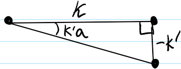
where the dependence on the scattering angle \(\textbf k\cdot\textbf k’=k^2\cos\theta\) can be made to appear explicitly by writing \(|\Delta\textbf k|^2=|\textbf k’-\textbf k|^2=2k^2(1-\cos\theta)=4k^2\sin^2\theta/2\) as evident geometrically in this \(\textbf k,\textbf k’\)-rhombus:
\[f(\theta)=\frac{2mg^2}{\hbar^2(4k^2\sin^2\theta/2+1/R^2)}\]
The differential cross-section for Yukawa scattering is then of course:
\[d\sigma=\frac{4m^2g^4}{\hbar^4(4k^2\sin^2\theta/2+1/R^2)^2}d\Omega\]
With cross-section given \(\sigma\) given by:
\[\sigma=\int d\sigma=\frac{16\pi m^2g^4R^2}{\hbar^4(4k^2+1/R^2)}\]
(note that the optical theorem would seem to predict \(\sigma=0\) because the scattering amplitude \(f(\theta)\in\textbf R\) is real-valued; this is not a contradiction, but rather a limitation of the Born series approximation which is implicit in all the computations we’ve been doing).
In particular, if one now lets the range \(R\to\infty\) of the Yukawa force to become long-range and \(g^2=\alpha\hbar c\), then one would seem to obtain the corresponding scattering amplitude, differential cross-section, and total cross-section for Rutherford scattering:
\[f(\theta)=\frac{\alpha}{2\bar{\lambda}k^2\sin^2\theta/2}\]
\[d\sigma=\frac{\alpha^4}{4\bar{\lambda}^2k^4\sin^4\theta/2}d\Omega\]
\[\sigma=\infty\]
Although we don’t have a classical analog of the scattering amplitude \(f(\theta)\), we did previously see a classical computation for the differential cross section \(d\sigma\) which one can check agrees with this first-order Born approximation from quantum scattering! (by trivial extension both the classical and quantum scattering calculations also agree that the Coulomb cross-section blows up \(\sigma=\infty\)). However, although ultimately it turns out that this is the correct answer for the differential-cross section \(d\sigma\), the method here of simply starting from the Yukawa potential and extending the range to \(R\to\infty\) is invalid.
Finally Doing Quantum Rutherford Scattering Correctly
To see why taking \(R\to\infty\) is invalid, here we finally calculate Rutherford scattering properly.
The scattering amplitude obtained earlier from a first-order Born approximation was thus wrong, though it’s mod-square was correct!
(make a spherical plot of the |f(theta)|^2 diff. cross section).
…