
Problem: Mobius transformations (also called fractional linear transformations) are maps \(\mathcal M:\textbf C\cup\{\infty\}\to\textbf C\cup\{\infty\}\) on the Riemann sphere \(\textbf C\cup\{\infty\}\) of the form \(\mathcal M(z):=\frac{az+b}{cz+d}\) for \(\det\begin{pmatrix}a&b\\c&d\end{pmatrix}\neq 0\). The purpose of this problem is to gain a deeper appreciation for just how versatile Mobius transformations can be.
a) Solve the equation \(\frac{5}{8}=\frac{11-3x}{4+7x}\) for \(x\in\textbf R\).
b) Solve the equation \(\frac{5}{8}=\frac{11-3x}{3+7x}\) for \(x\in\textbf R\).
c) Redo a) using the trick in b)
d) Decompose the following rational function into partial fractions:
\[\frac{x^2+15}{(x+3)^2(x^2+3)}\]
e) In general, the Mobius group is isomorphic to \(\cong\text{PGL}_2(\textbf C)\). This is incredibly powerful because it provides an explicit bridge between complex analysis and linear algebra. In this language, the question of which Mobius transformations are involutions \(\mathcal M^2=1\) boils down to which \(2\times 2\) complex invertible matrices \(M=\begin{pmatrix}a&b\\c&d\end{pmatrix}\) satisfy \(M^2=1\). By the Cayley-Hamilton theorem, any matrix with eigenvalues \(\lambda=\pm 1\) will satisfy such an equation…(but is that a sufficient condition?).
What’s the connection with unitary quantum logic gates on qubits? Give examples with 1D scattering (which is similar to Fresnel equations). Even for certain classes of intuitive \(2\)D matrices like rotations, what do the corresponding Mobius maps say? And also is there any connection between evaluating a Mobius map on some \(z\in\mathbf C\cup\{\infty\}\) and multiplying the corresponding matrix by a \(\mathbf C^2\) vector?
Solution:
a) Exploit the invariance under Mobius transformations of a suitable cross-ratio:
\[\frac{(x-0)(\infty-(-4/7))}{(x-\infty)(0-(-4/7))}=\frac{(5/8-11/4)(-3/7-\infty)}{(5/8-(-3/7))(11/4-\infty)}\]
\[-\frac{7x}{4}=\frac{-17/8}{59/56}\]
\[x=\frac{68}{59}\]
b) The trick is that any traceless Mobius transformation with \(a=-d\) is an involution. So the answer is just:
\[x=\frac{11-3\times(5/8)}{3+7\times(5/8)}=\frac{73}{59}\]
c) Since \(\text{lcm}(3,4)=12\), one has:
\[\frac{5}{8}=\frac{11-3x}{4+7x}\Rightarrow\frac{4}{3}\times\frac{5}{8}=\frac{4}{3}\times\frac{11-3x}{4+7x}\]
So:
\[x=\frac{4}{3}\times\frac{11-3\left(\frac{4}{3}\times\frac{5}{8}\right)}{4+7\left(\frac{4}{3}\times\frac{5}{8}\right)}=\frac{68}{59}\]
d) Remember that partial fractions may be viewed as just Mobius transformations with \(a=0\) (or powers thereof). In this case, that means:
\[\frac{x^2+15}{(x+3)^2(x^2+3)}=\frac{R_1}{x+3}+\frac{R_2}{(x+3)^2}+\frac{R_3}{x-\sqrt{3}i}+\frac{R_4}{x+\sqrt{3}i}\]
where the residues \(R_1,R_2,R_3,R_4\) may be calculated efficiently using the residue theorem (one may optionally prefer one’s residues to be real, in which case the last \(2\) terms should be combined as \(\frac{\tilde R_3x+\tilde R_4}{x^2+3}\); however as will be clear below it is actually very easy to get \(\tilde R_3,\tilde R_4\in\textbf R\) by simply summing \(\frac{R_3}{x-\sqrt{3}i}+\frac{R_4}{x+\sqrt{3}i}\) once the complex residues \(R_3,R_4\in\textbf C\) have been obtained; partial fraction composition is much easier decomposition!). To begin, it is helpful to complexify \(x\mapsto z\) everywhere:
\[\frac{z^2+15}{(z+3)^2(z^2+3)}=\frac{R_1}{z+3}+\frac{R_2}{(z+3)^2}+\frac{R_3}{z-\sqrt{3}i}+\frac{R_4}{z+\sqrt{3}i}\]
Now, suppose one wished to extract the residue at one of the simple poles, say \(R_1\). Then pick any contour in \(\textbf C\) that encloses only the corresponding simple pole, in this case at \(z=-3\) (strictly speaking \(z=-3\) is a double pole of the relevant function but that’s a technicality as far as computing \(R_1\) is concerned), and compute the corresponding contour integral on both sides, normalized by \(2\pi i\):
\[\frac{1}{2\pi i}\oint dz\frac{z^2+15}{(z+3)^2(z^2+3)}=\frac{1}{2\pi i}\oint dz\left(\frac{R_1}{z+3}+\frac{R_2}{(z+3)^2}+\frac{R_3}{z-\sqrt{3}i}+\frac{R_4}{z+\sqrt{3}i}\right)\]
On the right-hand side of course only the Mobius transformation with the simple pole at \(z=-3\) survives, leaving behind its residue:
\[R_1=\frac{1}{2\pi i}\oint dz\frac{(z^2+15)/(z^2+3)}{(z+3)^2}\]
By the generalized Cauchy integral formula, this is:
\[R_1=\frac{1}{1!}\left(\frac{d}{dz}\right)_{z=-3}\frac{z^2+15}{z^2+3}=\frac{1}{2}\]
By changing the contour to enclose the simple poles at \(z=\pm\sqrt{3}i\), one can similarly compute the residues \(R_3=1/(\sqrt{3}i-3)\) and \(R_4=-1/(3+\sqrt{3}i)\) (here just the vanilla Cauchy integral formula will do). This immediately leads to the residues \(\tilde R_3=-1/2\) and \(\tilde R_4=1/2\).
Finally to compute the “residue” \(R_2\) at the \(z=-3\) double pole, one simply has to convert it into a simple pole by multiplying through the whole equation by a factor of \((z+3)\):
\[\frac{z^2+15}{(z+3)(z^2+3)}=R_1+\frac{R_2}{z+3}+\frac{R_3(z+3)}{z-\sqrt{3}i}+\frac{R_4(z+3)}{z+\sqrt{3}i}\]
And now contour-integrate this around \(z=-3\):
\[R_2=\frac{(-3)^2+15}{(-3)^2+3}=2\]
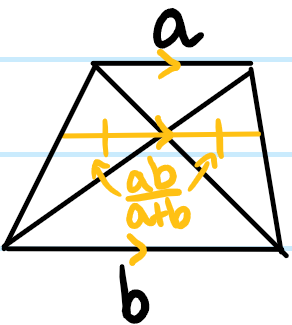
Problem: Prove that the diagonals of any trapezoid intersect at the harmonic mean of the \(2\) parallel sides of the trapezoid:
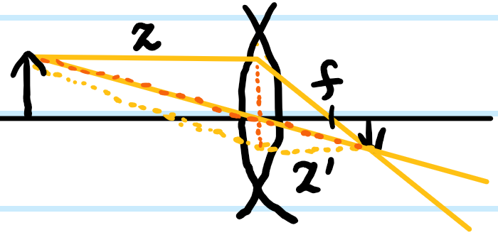
a) Apply this visualization to derive the thin lens imaging condition.
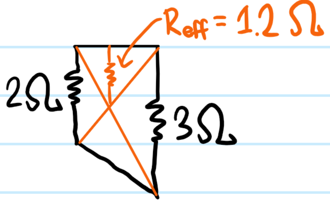
b) Apply this visualization to reformulate how resistors, capacitors, inductors and springs in parallel can be combined.
c) Apply this visualization to better understand the reduced mass of a \(2\)-body system.
Solution: The proof is simply a matter of similar triangles.
a) Clearly, one can construct a trapezoid with parallel sides of length \(z,z’>0\). But since the diagonals of the trapezoid must intersect at the center of the convex lens, it follows that \(1/f=1/z+1/z’\).
b) Since resistance \(R=\rho z/A_{\perp z}\propto z\) scales with the length \(z\) anyways, one can elevate the status of electric circuits from topology to geometry (see: crossed ladders problem):
Same reasoning can be applied to capacitors (provided one works with their elastance \(C^{-1}=z/\varepsilon A_{\perp z}\)) or inductors \(L=\mu n^2 A_{\perp z}z\) or even elastic springs (provided one works with their elasticity \(k^{-1}=z/EA_{\perp z}\)); in all cases, it is the signature linear \(\propto z\) behavior of the extensive constant that allows this to work.
c) Still trying to think about this one…perhaps \(2\) parallel uniformly massive rods of different lengths interacting gravitationally or otherwise with each other?
Problem: Extremize the function \(f(x)=\frac{x}{a}+\frac{b}{x}\).
Solution: The rigorous way to do this is to set \(f'(x)=\frac{1}{a}-\frac{b}{x^2}=0\Rightarrow x=\pm\sqrt{ab}\) is the geometric mean of \(a\) and \(b\). The quick and dirty way to do this is to just set the two terms in \(f(x)\) equal to each other:
\[\frac{x}{a}=\frac{b}{x}\Rightarrow x=\pm\sqrt{ab}\]
The intuition here is that whenever one is seeking to extremize the sum of an increasing function and a decreasing function, there is often a balancing act that happens between these terms that dictates where the extrema will lie, so up to numerical pre-factors of \(O(1)\) it is often possible to estimate the locations of such extrema without doing much work. Indeed, this is a common theme in physics (e.g. the healing length \(\xi\) of a Bose-Einstein condensate being set by the balance of kinetic and interaction energies \(\frac{\hbar^2}{2m\xi^2}=gn_0\Rightarrow\xi=\hbar/\sqrt{2mn_0g}\), the equilibrium of free energy \(F=E-TS\) being set by the balance between minimizing energy \(E\) and maximizing entropy \(S\) such as in Flory theory of polymers \(N\sim R^{3/5}\), etc.)
Problem: Solve the equation \(x^3=-\ln x\).
Solution: Here, the idea is to reverse-engineer the previous logic and convert this to an optimization problem \(f(x):=x^3-\ln x\). Then \(f'(x)=3x^2-\frac{1}{x}=0\Rightarrow x=1/3^{1/3}\approx 0.693\). In this case the exact answer turns out to be \(x=(W(3)/3)^{1/3}\approx 0.705\). They are close because \(W(3)\approx 1.05\approx 1\).
Problem: (something related to the above intuition, but instead of a sum, consider a product, and take the log to convert to a sum)