
The purpose of this post is to provide some examples of perturbation theory calculations in quantum mechanics by analyzing a specific perturbation called the Stark effect. For simplicity, we take as our quantum system a hydrogen atom with the usual non-relativistic two-body Hamiltonian:
\[H=\frac{P^2}{2\mu}-\frac{e^2}{4\pi\varepsilon_0|\textbf X|}\]
and corresponding non-relativistic energy spectrum \(E_n=-\frac{1}{2}\left(\frac{\alpha}{n}\right)^2\mu c^2\). We now apply a constant external electric field \(\textbf E_{\text{ext}}=E_{\text{ext}}\hat{\textbf k}\) which is not too strong \(0<E_{\text{ext}}\ll e^2/4\pi\varepsilon_0r^2_{\text{Bohr}}\) along the \(z\)-axis and ask how this perturbs the original energy spectrum \(E_n\) (one can of course also calculate how it will perturb the corresponding \(H\)-eigenstates \(|n,\ell,m_{\ell}\rangle\) but for now we won’t look too deeply into that).
Before delving into the math, it is always helpful to leverage some classical intuition to try and predict what effect the perturbation will have on the various unperturbed \(H\)-eigenstates \(|n,\ell,m_{\ell}\rangle\) as well as their energies \(E_n\). Classically, we expect the proton \(p^+\) in the nucleus to be tugged in the direction of \(\textbf E_{\text{ext}}\) along the positive \(z\)-axis while the electron \(e^-\) is tugged by an equal and opposite force along the negative \(z\)-axis. Thus, for \(H\)-eigenstates where the electron \(e^-\) position space wavefunction \(\langle\textbf x|n,l,m_{\ell}\rangle\) was more concentrated “above” the proton \(p^+\), the average electric dipole moment \(\textbf p\) would find itself anti-aligned relative to the electric field \(\textbf E_{\text{ext}}\), leading to a positive energy contribution \(-\textbf p\cdot\textbf E_{\text{ext}}>0\) so that the energy \(E_n\) of that \(H\)-eigenstate is expected to increase (one might object that the Coulomb potential energy \(V\) would decrease. By a similar logic, \(H\)-eigenstates where the \(e^-\) was predominantly “below” the proton \(p^+\) should experience a decrease in their energy \(E_n\).should this should increasing their electric dipole moment \(\textbf p\) and by extension their average Coulomb potential energy \(\langle V\rangle\), hence by the virial theorem also leading on average to an increased energy \(\langle H\rangle =\langle V\rangle/2\). It remains to be seen if quantum mechanics bears out these classical considerations!
The Stark perturbation \(\Delta H_{\text{Stark}}\) to the original Hamiltonian \(H\) due to the application of the external electric field \(\textbf E_{\text{ext}}\) arises physically from the coupling between the electric dipole moment \(\textbf p\) of the proton-electron pair defining the hydrogen atom and the external electric field \(\textbf E_{\text{ext}}\), i.e. \(\Delta H_{\text{Stark}}=-\textbf p\cdot\textbf E_{\text{ext}}=-(-e\textbf X)\cdot\textbf E_{\text{ext}}=eE_{\text{ext}}X_3\).
Case #1: Nondegenerate Perturbation Theory
The easiest Stark perturbation to compute pertains to the ground state \(|1,0,0\rangle\) of the hydrogen atom. The reason it’s the easiest is simply that there is only one unique ground state in hydrogen (caveat: we are working with non-relativistic quantum mechanics so we’ll pretend we don’t know about spin!). So for the \(n=1\) ground state there is no degeneracy to worry about (which is decisively not true for \(n>1\)!). The ground state \(|1,0,0\rangle\) of course initially possesses an unperturbed energy \(E_1\approx -13.6\text{ eV}\). Using the standard result of nondegenerate perturbation theory, the first-order correction \(\Delta E_1^{(1)}\) to the unperturbed ground state energy \(E_1\) is given by the expectation of the unperturbed ground state \(|1,0,0\rangle\) in the perturbation Hamiltonian \(\Delta H_{\text{Stark}}\):
\[\Delta E_1^{(1)}=\langle 1,0,0|\Delta H_{\text{Stark}}|1,0,0\rangle=-eE_{\text{ext}}\langle 1,0,0|X_3|1,0,0\rangle\]
Recall that rotational symmetry \([H,\textbf L]=\textbf 0\) automatically implies centrosymmetry \([H,\Pi]=0\) and so \(\Pi|n,\ell,m_{\ell}\rangle=(-1)^{\ell}|n,\ell,m_{\ell}\rangle\) have definite parity. It follows that the ground state \(|1,0,0\rangle\) has even parity \(\Pi|1,0,0\rangle=|1,0,0\rangle\) so we expect \(\langle 1,0,0|X_3|1,0,0\rangle=\langle 1,0,0|\Pi^{\dagger}X_3\Pi|1,0,0\rangle=-\langle 1,0,0|X_3|1,0,0\rangle\) (where we’ve used the fact that \(\textbf X\) is a vector operator), thus to first-order \(\Delta E_1^{(1)}=0\) and the ground state energy \(E_1\) is unaffected (notice the above argument would have been equally valid if the ground state were to have odd parity! Thus, the key is not which parity it had, but that it had a definite parity at all). Instead, the Stark perturbation only affects the ground state energy \(E_1\) at second-order \(\Delta E_1^{(2)}\neq 0\) which is why this is an example of the so-called quadratic Stark effect.
To compute the second-order correction \(\Delta E_1^{(2)}\), we need to calculate:
\[\Delta E_1^{(2)}=-e^2E_{\text{ext}}^2\sum_{n=2}^{\infty}\sum_{\ell=0}^{n-1}\sum_{m_{\ell}=-\ell}^{\ell}\frac{|\langle n,\ell,m_{\ell}|X_3|1,0,0\rangle|^2}{E_n-E_1}\]
Since \(X_3\) is already the \(T^1_0\) spherical component of the rank-\(1\) tensor operator \(\textbf X\) (since it’s a vector operator!), the Wigner-Eckart theorem asserts that the matrix element \(\langle n,\ell,m_{\ell}|X_3|1,0,0\rangle\) is proportional to the Clebsch-Gordan coefficient \(\langle n,\ell,m_{\ell}|\otimes\langle 1,0,0|1,0\rangle\). In particular, one has the usual angular momentum addition selection rules \(0=m_{\ell}+0\) and \(|\ell-0|\leq 1\leq\ell+0\), so the only non-vanishing matrix elements are those with \(\ell=1,m_{\ell}=0\) (put another way, the only states that mix with the ground state \(|1,0,0\rangle\) are those of the form \(|n,1,0\rangle\)). The second-order energy correction \(\Delta E_1^{(2)}\) to the ground state \(|1,0,0\rangle\) simplifies to a single infinite series:
\[\Delta E_1^{(2)}=-e^2E_{\text{ext}}^2\sum_{n=2}^{\infty}\frac{|\langle n,1,0|X_3|1,0,0\rangle|^2}{E_n-E_1}\]
where, if you want the details of that sum, see here. The point is \(\Delta E_1^{(2)}<0\). Classically, the external electric field \(\textbf E_{\text{ext}}\) polarizes the hydrogen atom with electric dipole moment \(\textbf p=\alpha\textbf E_{\text{ext}}\) with \(\alpha>0\) the atomic polarizability, so it makes sense that the perturbation \(V_{\text{Stark}}=-\textbf p\cdot\textbf E_{\text{ext}}=-\alpha E_{\text{ext}}^2<0\) is both negative and comes in at quadratic order \(V_{\text{Stark}}=O_{E_{\text{ext}}\to 0}(E_{\text{ext}}^2)\).
Case #2: Degenerate Perturbation Theory
Now we compute the Stark perturbation for the \(n=2\) states. Recall that in the hydrogen atom, the \(n\)-th energy level \(E_n\) is associated with an \(\sum_{\ell=0}^{n-1}(2\ell+1)=n^2\)-dimensional degenerate \(H\)-eigensubspace. For \(n=1\), \(1^2=1\) so we have a single non-degenerate ground state \(|1,0,0\rangle\) as before. However, for \(n=2\) we have \(2^2=4\) degenerate states \(|2,0,0\rangle,|2,1,-1\rangle,|2,1,0\rangle\) and \(|2,1,1\rangle\) (in chemistry lingo, the \(2s\)-wave and the three \(2p\)-waves). As usual, we look for eigenstates of the perturbation Hamiltonian \(\Delta H_{\text{Stark}}\biggr|_{\ker(H-E_2 1)}\) restricted to the degenerate \(E_2\)-eigensubspace \(\ker(H-E_2 1)=\text{span}_{\textbf C}|2,0,0\rangle,|2,1,-1\rangle,|2,1,0\rangle,|2,1,1\rangle\) of the unperturbed Hamiltonian \(H\) since such eigenstates are automatically eigenstates of the perturbed Hamiltonian \(H+\Delta H_{\text{Stark}}\)! The matrix elements of \(\Delta H_{\text{Stark}}\biggr|_{\ker(H-E_2 1)}\) in the obvious basis \(|2,0,0\rangle,|2,1,-1\rangle,|2,1,0\rangle,|2,1,1\rangle\) may be determined through parity considerations for the diagonal elements and Wigner-Eckart selection rule considerations for the off-diagonal elements:
\[\left[\Delta H_{\text{Stark}}\biggr|_{\ker(H-E_2 1)}\right]_{|2,0,0\rangle,|2,1,-1\rangle,|2,1,0\rangle,|2,1,1\rangle}^{|2,0,0\rangle,|2,1,-1\rangle,|2,1,0\rangle,|2,1,1\rangle}=-3er_{\text{Bohr}}E_{\text{ext}}\begin{pmatrix}0&0&1&0\\0&0&0&0\\1&0&0&)\\0&0&0&0\end{pmatrix}\]
Thus with only (3\) distinct eigenvalues \(-3er_{\text{Bohr}}E_{\text{ext}},0,3er_{\text{Bohr}}E_{\text{ext}}\) representing the degeneracy-lifting energy corrections that need to be made to the degenerate energy \(E_2\) (actually though, having an eigenvalue of \(0\) means no energy correction is made!). Thus, the Stark perturbation lifts the degeneracy among the states \(|2,0,0\rangle\) and \(|2,1,0\rangle\) by mixing them into \(2\) “\(sp\) hybrid waves” with equiprobable “\(50\%\) \(s\)-character” and “\(50\%\) \(p\)-character”.
\[\{|2,0,0\rangle,|2,1,0\rangle\}\mapsto\biggr\{\frac{|2,0,0\rangle-|2,1,0\rangle}{\sqrt{2}},\frac{|2,0,0\rangle+|2,1,0\rangle}{\sqrt{2}}\biggr\}\]
Note that it doesn’t really make sense to say specifically which of the unperturbed states \(|2,0,0\rangle,|2,1,0\rangle\) “became” which of the two new hybrid states. It only makes sense to say that they mixed. The other two \(p\)-waves \(|2,1,-1\rangle,|2,1,1\rangle\) remain degenerate/”unhybridized” \(p\)-waves.
\[\{|2,1,-1\rangle,|2,1,1\rangle\}\mapsto\{|2,1,-1\rangle,|2,1,1\rangle\}\]
Although the energy corrections to \(E_2\) scaled linearly with \(E_{\text{ext}}\) (thus, this is called the linear Stark effect), the new eigenstates are completely independent of \(E_{\text{ext}}\)! Even the slightest stray electric field in the lab evidently causes the hydrogen atom to prefer the probabilistic superposition. Diagramatically, the Stark perturbation as a function of the external electric field strength for the states considered so far looks like:
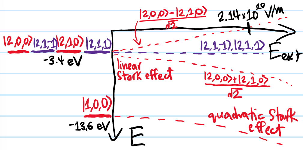
I mentioned this already, but I just wanted to re-emphasize that “degenerate perturbation theory” is a misnomer because the energies have been computed exactly rather than perturbatively! That’s it, those are the exact linear Stark effect energies! It is interesting to try and think about why these results make sense classically.
From an experimental physics perspective, the Stark effect enables one to “sniff out” degeneracies in the Hamiltonian \(H\) of an initially “highly symmetric” quantum system simply through the application of an external electric field \(\textbf E_{\text{ext}}\) (which breaks that symmetry and therefore the degeneracy). If the agent causing the external electric field \(\textbf E_{\text{ext}}\) is say another atom, then roughly speaking the Stark effect (specifically the linear Stark effect part where the lowest-energy lifted state \((|2,0,0\rangle+|2,1,0\rangle)\sqrt{2}\) is maximally delocalized) also explains why conductors work.