
Problem: Before developing FGR, it is first necessary to lay out as a prerequisite the general framework of time-dependent perturbation theory (FGR is then a special case thereof). To this effect, consider the usual (Schrodinger picture) Hamiltonian decomposition \(H=H_0+V\), and obtain the “fundamental theorem of (\(1^{\text{st}}\)-order) time-dependent perturbation theory” for the transition amplitude between an initial (Schrodinger picture) \(H_0\)-eigenstate \(|i\rangle\) at \(t=0\) and a final (Schrodinger picture) \(H_0\)-eigenstate \(|f\rangle\) with distinct energies \(E_f\neq E_i\) as a function of the elapsed time \(t\):
\[\langle f|\mathcal T\exp\left(-\frac{i}{\hbar}\int_0^tdt’H(t’)\right)|i\rangle\sim h^{-1}V_{fi}(\omega_{fi})*_{\omega_{fi}}e^{i\omega_{fi}t/2}t\text{sinc}\frac{\omega_{fi}t}{2}\]
where \(\hbar\omega_{fi}:=E_f-E_i\), \(V_{fi}(\omega_{fi}):=\langle f|V(\omega_{fi})|i\rangle\) and the linear response Fourier transform convention is being used:
\[V(\omega):=\int_{-\infty}^{\infty}dte^{i\omega t}V(t)\]
Solution: First one has to establish the following exact decomposition lemma for the time evolution operator under the perturbed Hamiltonian \(H\) (prove by showing both sides obey \(i\hbar\dot U=HU\) with \(U(0)=1\)):
\[\mathcal T\exp\left(-\frac{i}{\hbar}\int_0^tdt’H(t’)\right)=\exp\left(-\frac{iH_0t}{\hbar}\right)\mathcal T\exp\left(-\frac{i}{\hbar}\int_0^tdt’V_{/H_0}(t’)\right)\]
(aside: one can commute the \(2\) time evolutions at the expense of using the retarded time:
\[=\mathcal T\exp\left(-\frac{i}{\hbar}\int_0^tdt’V_{/H_0}(t’-t)\right)\exp\left(-\frac{iH_0t}{\hbar}\right)=\mathcal T\exp\left(-\frac{i}{\hbar}\int_{-t}^0dt’V_{/H_0}(t’)\right)\exp\left(-\frac{iH_0t}{\hbar}\right)\]
Note such decompositions exist only because the time integral begins at a finite \(t=0\) rather than e.g. \(t=-\infty\) as encountered in scattering theory).
Taking the matrix element of both sides in the \(H_0\)-eigenbasis, the free evolution piece \(\exp\left(-\frac{iH_0t}{\hbar}\right)\) contributes an irrelevant phase \(e^{-iE_ft/\hbar}\) when acting on the bra \(\langle f|\) since \(H_0\) cannot promote transitions between its own eigenstates; later when taking the mod-square of the transition amplitude to obtain a transition probability, this will drop out.
At this point, one employs the key step of (\(1^{\text{st}}\)-order) time-dependent perturbation theory, which is to Dyson-expand the time-ordered exponential to \(1^{\text{st}}\)-order (the word “order” here is being used in \(2\) different senses!):
\[\sim \langle f|1-\frac{i}{\hbar}\int_0^tdt’V_{/H_0}(t’)|i\rangle\]
Since \(E_f\neq E_i\) and \(H_0\) is Hermitian, it follows \(\langle f|i\rangle=0\) are orthogonal so the transition amplitude becomes:
\[\sim\hbar^{-1}\int_0^tdt’\langle f|V_{/H_0}(t’)|i\rangle=\hbar^{-1}\int_0^tdt’e^{i\omega_{fi}t’}\langle f|V(t’)|i\rangle\]
(aside: why not just Dyson-expand the original time-evolution operator \(\mathcal T\exp\left(-\frac{i}{\hbar}\int_0^tdt’H(t’)\right)\)? Answer: because it is \(V\) that is weak, not \(H=H_0+V\)! This simple observation motivates the whole point of using the interaction picture in the first place!)
At this point, the integral is recognized as a \([0,t]\)-windowed Fourier transform of \(\langle f|V(t)|i\rangle\), so by interpreting \(\int_0^tdt’=\int_{-\infty}^{\infty}dt'[0\leq t’\leq t]\) with a top-hat filter and using the convolution theorem, one arrives at the stated result (note that with this F.T. convention, there is a factor of \(2\pi\) in the convolution theorem that makes \(\hbar\mapsto h=2\pi\hbar\)).
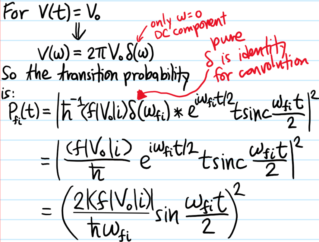
Problem: Suppose that \(V(t)=V_0\) is time-independent. Show that the transition probability between arbitrary \(H_0\)-eigenstates \(|i\rangle,|f\rangle\) undergoes Rabi oscillations:
\[p(t|\omega_{fi},V_0)=\left(\frac{2|\langle f|V_0|i\rangle|}{\hbar\omega_{fi}}\sin\frac{\omega_{fi}t}{2}\right)^2\]
Solution: This one leads to a “Fraunhofer single-slit”:
Problem: Instead of just a single DC component at \(\omega=0\), now let the spectrum of the perturbation \(V\) be monochromatic at some frequency \(\omega\neq 0\); due to Hermiticity requirements, such a perturbation must be of the form:
\[V(t)=V_0e^{i\omega t}+V_0^{\dagger}e^{-i\omega t}\]
leading to a Hermitian “Fraunhofer double-slit” spectrum:
\[V(\omega_{fi})=2\pi(V_0\delta(\omega_{fi}+\omega)+V_0^{\dagger}\delta(\omega_{fi}-\omega))\]
In this case, what does the transition probability become?
Solution:
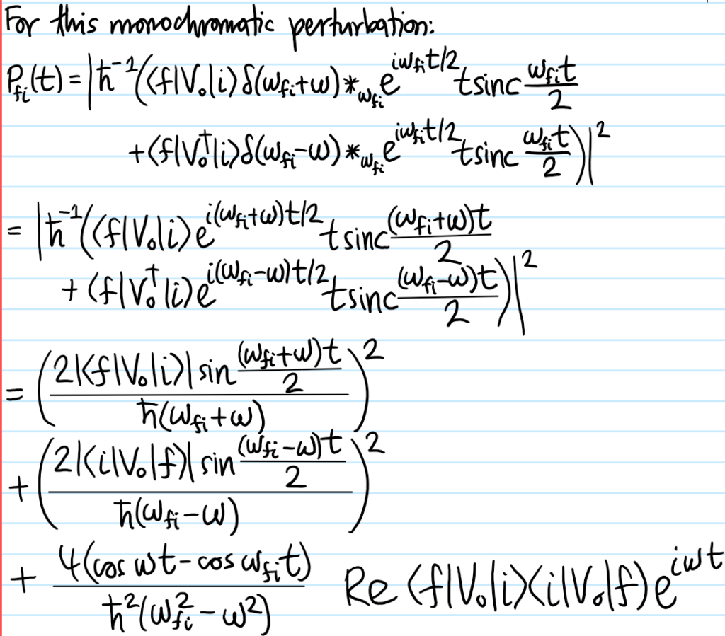
which correspond to the processes of stimulated absorption and emission.
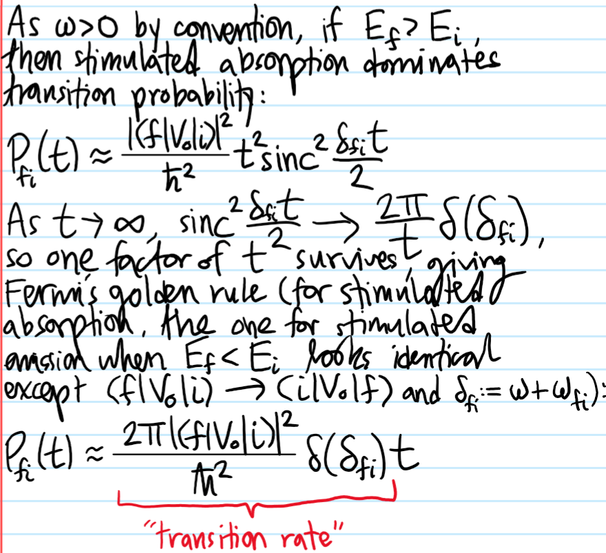
Problem: Show that:
\[\lim_{t\to\infty}t\text{sinc}^2(\omega t)=\pi\delta(\omega)\]
hence for large \(t\), one may approximate \(\text{sinc}^2(\omega t)=\pi\delta(\omega t)\) (or more concisely, \(\text{sinc}^2=\pi\delta\)). Using this lemma, establish Fermi’s golden rule for the “transition rate”:
\[\dot{p}(t|E_{fi},V)=\frac{2\pi}{\hbar}|\langle f|V|i\rangle|^2g_*(E_{fi})\]
Solution:
Problem: What is Fermi’s useful golden rule for stimulated absorption?
Solution: Instead of a discrete final \(H_0\)-eigenstate \(|f\rangle\), there should be a continuum (or in practice a quasi-continuum) of final states described by a density of \(H_0\)-eigenstates \(g_{f,H_0}(E_f)\). The useful form of Fermi’s golden rule for the transition rate into any of these energetically compatible \(H_0\)-eigenstates is then:
\[P_{fi}(t)\approx\frac{2\pi|\langle f|V_0|i\rangle|^2}{\hbar}g_{f,H_0}(E_f=E_i+\hbar\omega)\]
where a factor of \(\hbar\) has been (optionally) absorbed to have an energy rather than angular frequency argument in the density of states. Of course, a similar useful form of Fermi’s golden rule holds for stimulated emission.
Problem: What are the \(3\) key assumptions of Fermi’s golden rule (FGR)?
Solution: The \(3\) key assumptions are:
Assumption #\(1\): Weak coupling \(V(t)\) (several ways to formalize this).
Assumption #\(2\): Continuum (or in practice quasicontinuum) of final scattering \(H_0\)-eigenstates to transition into, hence described by a density of states \(g_{f,H_0}(E_f)\).
Assumption #\(3\): Intermediate time window (this leads to the idea of the emergence and subsequent breakdown of FGR as a function of time \(t\)).
In most quantum mechanics textbooks, Assumption #\(1\) tends to be emphasized clearly by the fact that one is doing (time-dependent) perturbation theory. Assumption #\(2\) is present in Fermi’s useful golden rule, so in that sense is a bit optional. Finally, Assumption #\(3\) tends to be obscured, and sometimes omitted entirely, but is absolutely critical.
Problem: Elaborate on the importance of Assumption #\(3\).
Solution: The fact that there should be a lower bound on \(t\) makes sense, as enough time needs to pass for the \(\text{sinc}^2\) to actually look like the \(\delta\) as one of the key steps above. However, at the same time the notion of \(t\to\infty\) is a bit artificial, and for one clearly cannot be strictly correct since otherwise the transition probability \(P_{fi}(t)\propto t\) would eventually exceed \(1\).
More quantitatively, if one (optionally) defines a notion of Rabi frequency in the usual way \(\hbar\Omega_{fi}/2:=|\langle f|V_0|i\rangle|\), then it’s clear from the earlier formula for the transition probability that, taking the \(t\to 0\) limit rather than \(t\to\infty\), it instead takes off quadratically in time \(t\) as \(P_{fi}(t)=\Omega_{fi}^2t^2/4\) before the emergence of the linear-in-\(t\) FGR regime.
Meanwhile, in the large-\(t\) limit, if one drives too strongly then of course perturbation theory breaks down and instead one would get Rabi oscillations or something like that. So the exact regime of validity of FGR is a much richer and subtler topic than it seems at first. See the paper of Micklitz et al. and the paper of Chen et al. for more details.
(aside: a scattering amplitude is simply a transition amplitude between \(2\) asymptotic scattering \(H_0\)-eigenstates; thus the term “transition amplitude” is more general, referring to the probability amplitude of an \(H_0\)-measurement at time \(t\) to yield the energy \(E_f\) given the quantum system was, at time \(t=0\), in the \(H_0\)-eigenstate \(E_i\)).
Problem: Explain under what conditions in a scanning tunneling spectroscopy experiment, the differential conductance \(dI/d\phi\propto g_{s}(E=e\phi)\).
Solution: Assuming the \(3\) conditions of Fermi’s golden rule are met, one has to integrate the joint density of states (a convolution) \(g_{t\to s}(E):=\int dE’g_{t}(E-E’)g_{s}(E’)\):
\[I(\phi)=\frac{2\pi}{\hbar}\int_0^{\phi}dE g_{t}(E)g_{s}(E)|\langle E|V|E\rangle|^2\]
thus:
\[\frac{dI}{d\phi}=\frac{2\pi}{e\hbar}g_{t}(e\phi)|\langle e\phi|V|e\phi\rangle|^2\]
Problem: A hydrogen atom in its \(s\)-wave bound ground state is ionized by light of frequency \(\omega\). Calculate the FGR transition rate to the continuum of asymptotically free scattering states (this is a simple model of the photoelectric effect).
Solution: A qualitative sketch of the calculation: first, ignore quantization of the EM field (valid for e.g. a laser) by imposing a suitable vector potential such as \(\textbf A\propto e^{i(\textbf k\cdot\textbf x-\omega_{\textbf k}t)}\) for the usual planar EM wave. The perturbation Hamiltonian \(V(t)\) is determined by expanding to first-order the usual minimally-coupled Hamiltonian \(H\) for a charge \(q=-e\) in an electromagnetic field. Since this is absorption rather than stimulated emission, compute the matrix element of the appropriate term between the hydrogen atom ground state \(|1,0,0\rangle\) and the free \(e^-\) state \(|\textbf k\rangle\) (where recall that the density of such free states is \(g_{f,H_0}(E)\propto\sqrt E\)).
Problem: (to be added, dipole approximation demonstration that rates of stimulated absorption/emission are same, and the first-order p.t. expression for that rate).
Solution: Fermi’s golden rule applied to a monochromatic perturbation (should this be treated as another assumption?), but for a more general spectrum, even transitions between discrete bound \(H_0\)-eigenstates are possible, e.g. atom bathing in a photon gas. To compute the stimulated absorption/emission rates \(\Gamma_a,\Gamma_e\) it is common to employ a so-called dipole approximation (though in this context I feel a better name would be long-wavelength approximation or even just cold approximation; note also that this is a further approximation on top of all the other approximations that have already been made before this) in which the typical wavelength \(\lambda\gg r_B\) of photons \(\gamma\) in the thermal bath is much longer than the Bohr radius \(r_B\) representing the typical length scale of atoms. Essentially what this means is that the vector potential \(\textbf A\sim e^{i(\textbf k_{\text{ext}}\cdot\textbf x-\omega_{\text{ext}} t)}\approx e^{-i\omega_{\text{ext}}t}\) is approximately spatially uniform for \(\textbf k_{\text{ext}}\cdot\textbf x\ll 1\) for \(\textbf x\) ranging over the atom, and therefore the time-dependent perturbation to the atom just has the form \(\Delta\tilde H(t)=e\textbf E_{\text{ext}}(t)\cdot\sum_{e^-}\textbf X_{e^-}\) where \(e\sum_{e^-}\textbf X_{e^-}\) is the net electric dipole moment of the atom, hence the name “dipole approximation”. Chugging this into Case #\(2\) of Fermi’s golden rules, one can compute the rates of stimulated absorption and emission to be equal and given by:
\[\Gamma_{1\to 2}=\Gamma_{2\to 1}=\frac{\pi e^2}{3\varepsilon_0\hbar^2}\left|\sum_{e^-}\langle 2|\textbf X_{e^-}|1\rangle\right|^2g(\Delta E_{12})\]
Note that non-relativistic quantum mechanics predicts that atoms can only undergo stimulated absorption or stimulated emission. In particular, non-relativistic quantum mechanics predicts that there are no such things as “spontaneous absorption” or “spontaneous emission” \(\Gamma_{1\to 2}^*=\Gamma_{2\to 1}^*=0\) where an atom can undergo a transition between \(\tilde H\)-eigenstates in the absence \(\textbf E_{\text{ext}}=\textbf B_{\text{ext}}=\textbf 0\) of external electromagnetic fields/photons (because the non-relativistic Schrodinger equation asserts that the \(t\)-evolution of \(\tilde H\)-eigenstates is to stay right where they are rather than hopping to other \(\tilde H\)-eigenstates). Indeed, it turns out there is no such thing as “spontaneous absorption” \(\Gamma_{1\to 2}^*\), but there can be spontaneous emission \(\Gamma_{2\to 1}^*\neq 0\). This phenomenon only arises once one quantizes the classical, smooth electromagnetic field \((\textbf E,\textbf B)\). When this is done, it is found that spontaneous emission is possible due to interactions between the atom and zero-point fluctuations of the quantum electromagnetic field, but to delve deeper would be the subject of quantum electrodynamics.
Nevertheless, Einstein was able to compute the rate of spontaneous emission \(\Gamma_{2\to 1}^*\) without knowing anything about the quantization of the electromagnetic field. Or more precisely, Einstein showed that if one could calculate the stimulated emission rate \(\Gamma_{2\to 1}\), then one would also get the spontaneous emission rate \(\Gamma_{2\to 1}^*\) “for free” since he found that the two were proportional to each other and what that proportionality constant was.
Einstein’s Statistical Argument for Spontaneous Emission
Consider any \(2\) energy levels \(E_1<E_2\) in an atom of degeneracies \(\Omega_1,\Omega_2\) with number of electrons \(N_1,N_2\) respectively.
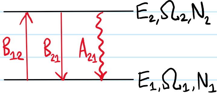
Then in general, one heuristically expects probabilistic kinetics of the form (ASIDES: what happens if one also adds a “spontaneous absorption” term \(A_{12}N_1\) among the rate terms? And also, need to explicitly related the \(\Gamma\)-transition rates above in Fermi’s golden rule with this triplet of Einstein coefficients):
Consider a \(2\)-level system \(\mathcal H=\text{span}_{\mathbf C}|0\rangle,|1\rangle\cong\mathbf C^2\) in steady state thermal equilibrium \(\dot N_0=\dot N_1=0\) with a photon gas at temperature \(T\). The populations \(N_0,N_1\) of the \(2\) levels are Boltzmann distributed so that in particular \(N_0/N_1=g_0e^{\beta\hbar\omega_0}/g_1\) for \(\hbar\omega_0=E_1-E_0>0\). Meanwhile, the energy density of the photon gas per unit angular frequency \(d\omega\) is \(\frac{1}{c}\times\frac{2}{(2\pi)^3}4\pi\left(\frac{\omega}{c}\right)^2\frac{\hbar\omega}{e^{\beta\hbar\omega}-1}=\frac{\hbar\omega^3}{\pi^2c^3}\frac{1}{e^{\beta\hbar\omega}-1}\). The \(2\)-level system and the photon gas interact via \(3\) channels: stimulated absorption (rate \(B_{01}\frac{\hbar\omega_0^3}{\pi^2c^3}\frac{1}{e^{\beta\hbar\omega_0}-1}N_0\)), stimulated emission (rate \(B_{10}\frac{\hbar\omega_0^3}{\pi^2c^3}\frac{1}{e^{\beta\hbar\omega_0}-1}N_1\)), and spontaneous emission (rate \(A_{10}N_1\)), where the \(3\) Einstein coefficients \(B_{01},B_{10},A_{10}>0\) are each \(\omega_0\)-dependent (there is no such thing as “spontaneous absorption” \(A_{01}=0\)).
Equating the rate of \(01\) processes with the rate of \(10\) processes:
\[B_{01}\frac{\hbar\omega_0^3}{\pi^2c^3}\frac{1}{e^{\beta\hbar\omega_0}-1}N_0=B_{10}\frac{\hbar\omega_0^3}{\pi^2c^3}\frac{1}{e^{\beta\hbar\omega_0}-1}N_1+A_{10}N_1\]
\[\frac{\hbar\omega_0^3}{\pi^2c^3}\frac{1}{e^{\beta\hbar\omega_0}-1}=\frac{A_{10}}{B_{10}}\frac{1}{\frac{g_0B_{01}}{g_1B_{10}}e^{\beta\hbar\omega_0}-1}\]
Because this result must hold for arbitrary equilibrium temperatures \(\beta\), one can just “pattern-match” (crucially, this is only possible thanks to Einstein’s introduction of spontaneous emission \(A_{10}\neq 0\) into the model!):
\[g_0B_{01}=g_1B_{10}\]
\[\frac{A_{10}}{B_{10}}=\frac{\hbar\omega_0^3}{\pi^2 c^3}\]
The first equality simply asserts that the transition rates \(\Gamma_{01}=\Gamma_{10}\) are equal (where \(\Gamma_{ij}:=g_iB_{ij}\)), which follows on the grounds that stimulated absorption of a photon of energy \(-E\) is equivalent to stimulated emission of a photon of energy \(E\) because the relevant Hamiltonian \(H\sim e^{i\omega_0 t}+e^{-i\omega_0 t}\) is Hermitian.
The second equality is the genuinely novel prediction (agreeing with the answer obtained from more rigorous QED calculations; here, Einstein implicitly quantizes the EM field by invoking the Planck distribution for the photon gas in the derivation). It’s nice because it provides a bridge to get from the \(B\)’s (which can be computed using standard dipole approximation/time-dependent perturbation theory) to the \(A\) (which outside of QED would not be computable otherwise). When this is done, one finds the lifetime \(\tau_{10}:=1/A_{10}\) of the excited state \(|1\rangle\) is given by:
\[\tau_{10}\approx \frac{3m_{e^-}c^3}{4\hbar\omega^3_0a_0}\]