Quantumplations

Problem: Write down the Lagrangian \(L\) of a nonrelativistic classical point charge \(q\) of mass \(m\) moving in an electromagnetic field. Justify it.

Solution: \(L=T-V\) as usual where the nonrelativistic kinetic energy \(T=m|\dot{\mathbf x}|^2/2\) (if it were relativistic then \(T=-mc^2/\gamma_{|\dot{\mathbf x}|}\)) and the velocity-dependent electromagnetic potential energy \(V\) must be written in terms of the electromagnetic gauge potentials:

\[V=q(\phi(\mathbf x,t)-\dot{\mathbf x}\cdot\mathbf A(\mathbf x,t))\]

The ultimate justification for this choice of \(L\) is that the corresponding Euler-Lagrange equations reproduce the nonrelativistic Lorentz force law:

\[m\ddot{\mathbf x}=q(\mathbf E(\mathbf x,t)+\dot{\mathbf x}\times\mathbf B(\mathbf x,t))\]

where \(\textbf E=-\frac{\partial\phi}{\partial\textbf x}-\frac{\partial\textbf A}{\partial t}\) and \(\textbf B=\frac{\partial}{\partial\textbf x}\times\textbf A\).

However, it can be motivated by the fact that the interaction portion of the action \(S_V=-q\int d\tau v^{\mu}A_{\mu}=-\int dt V\) is manifestly a Lorentz scalar so in particular by time dilation \(dt/d\tau=\gamma\) one recovers the above form of \(V\).

Problem: Compute the corresponding Hamiltonian \(H\) of the nonrelativistic charge \(q\) of mass \(m\) in the electromagnetic field. Hence, derive the minimal coupling rule.

Solution: One has the conjugate momentum \(\mathbf p=\frac{\partial L}{\partial\mathbf x}=m\dot{\mathbf x}+q\mathbf A(\mathbf x,t)\) which in particular is not the usual \(m\dot{\mathbf x}\) momentum due to the additional magnetic contribution \(q\mathbf A\) from the velocity-dependent magnetic potential. The Hamiltonian can thus be computed to obey the minimal coupling rule \(\mathbf p\mapsto\mathbf p-q\mathbf A\):

\[H:=\dot{\textbf x}\cdot\textbf p-L=\frac{|\textbf p-q\textbf A(\textbf x,t)|^2}{2m}+q\phi(\textbf x,t)\]

Problem: Comment on how the Lagrangian \(L\) and Hamiltonian \(H\) behave under electromagnetic gauge transformations \(A^{\mu}\mapsto A^{\mu}+\partial^{\mu}\Gamma\).

Solution: \(L\) is not gauge invariant, rather accumulating a total time derivative \(L\mapsto L-q\dot{\Gamma}\). On the other hand, \(H\) changes by a partial time derivative \(H\mapsto H+q\frac{\partial\Gamma}{\partial t}\). The equations of motion (whether in the form of Euler-Lagrange or Hamilton) are of course gauge invariant since \(\mathbf E,\mathbf B\) are gauge invariant.

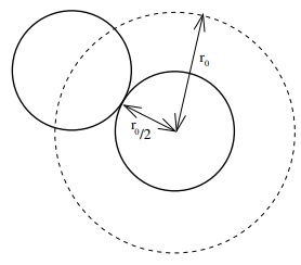
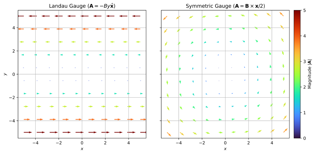
Problem: A simple case of the above formalism consists of a non-relativistic point charge \(q\) of mass \(m\) in a uniform magnetic field, thus \(\mathbf E=\mathbf 0\) (hence \(\phi=0\)) and \(\mathbf B=B\hat{\mathbf z}\). What are some suitable choices of the gauge field \(\mathbf A\)?

Solution: Physically, one is looking for a “flow field” \(\mathbf A(\mathbf x)\) whose vorticity will generate a \(\textbf B=\frac{\partial}{\partial\textbf x}\times\textbf A\) that points uniformly along \(z\). The \(2\) obvious ways to set this up are either in a “river” manner like \(\mathbf A=-By\hat{\mathbf x}\) or \(\mathbf A=Bx\hat{\mathbf y}\) (both examples of the Landau gauge) or in a “whirlpool” manner like \(\mathbf A=\mathbf B\times\mathbf x/2\) (called the symmetric gauge, cf. familiar fluid mechanics result \(\frac{\partial}{\partial\mathbf x}\times(\boldsymbol{\omega}\times\mathbf x)=2\boldsymbol{\omega}\)).

Problem: Now assume the point charge is a quantum particle and begin by working in the Landau gauge \(\mathbf A_L=-By\hat{\mathbf x}\). Diagonalize the corresponding Hamiltonian \(H=|\mathbf P-q\mathbf A_L|^2/2m\).

Solution: Expanding and completing the square:

\[H=\frac{P_y^2}{2m}+\frac{m\omega_B^2}{2}\left(Y+\frac{p_x}{m\omega_B}\right)^2+\frac{p_z^2}{2m}\]

where \(p_x,p_z\in\mathbf R\) are the momentum eigenvalues in the \(x\) and \(z\) directions since \([H,P_x]=[H,P_z]=0\) and \(\omega_B=qB/m\) is the classical cyclotron frequency. Meanwhile, in the \(y\)-direction, the Hamiltonian is identical to that of a (displaced) \(1\)D quantum harmonic oscillator with natural frequency \(\omega_B\); this defines the corresponding characteristic length scale \(\ell_B=\sqrt{\hbar/m|\omega_B|}=\sqrt{\hbar/|q|B}\) (called the magnetic length) and characteristic momentum scale \(p_B=\sqrt{\hbar m|\omega_B|}=\sqrt{\hbar |q|B}\) of the oscillator. The energies (called Landau levels) are:

\[E_{n,p_z}=\hbar\omega_B(n+1/2)+\frac{p_z^2}{2m}\]

and (not gauge-invariant) position-space wavefunctions:

\[\psi_{n,p_x,p_z}(x,y,z)\sim e^{i(p_xx+p_zz)/\hbar}H_n\left(\frac{y+p_x/m\omega_B}{\ell_B}\right)e^{-(y+p_x/m\omega_B)^2/2\ell_B^2}\]

Problem: Show that the \(n^{\text{th}}\) Landau level has degeneracy \(\dim\ker(H-E_{n,p_z=0}1)=\Phi_{\mathbf B}/\Phi_{\mathbf B,0}\) with \(\Phi_{\mathbf B}\) the magnetic flux through the plane perpendicular to \(\mathbf B\) and \(\Phi_{\mathbf B,0}=h/|q|\) the quantum of magnetic flux.

Solution: The degeneracy arises from the fact that \(E_{n,p_z=0}\) doesn’t depend on the \(p_x\) eigenvalue even though \(\psi_{n,p_x,p_z=0}\) does. If the system were infinitely large, then \(p_x\in\mathbf R\) would cause each Landau level to be uncountably degenerate; therefore, assume the system lives in a rectangle of dimensions \(L_x\times L_y\) (as \(p_z=0\) the system is effectively confined to the \(xy\)-plane). Then \(p_x\in\hbar\frac{2\pi}{L_x}\mathbf Z\) is quantized, which leads to quantization of the oscillator’s equilibrium \(y_0=-p_x/m\omega_B\in\frac{h}{m\omega_BL_x}\mathbf Z\) with adjacent equilibria separated by \(\Delta y_0=\frac{h}{m|\omega_B|L_x}\). Since this must lie in an interval of width \(L_y\), one obtains the degeneracy:

\[\dim\ker(H-E_{n,p_z=0}1)=\frac{L_y}{\Delta y_0}=\frac{\Phi_{\mathbf B}}{\Phi_{\mathbf B,0}}\]

since \(\Phi_{\mathbf B}=BL_xL_y\); note the result is independent of mass \(m\), independent of the sign of the charge \(q\), and also independent of \(n\in\mathbf N\), indicating all Landau levels are equally degenerate. Furthermore, if one plugs some numbers in (e.g. \(B=1\text{ T}\) for an electron or proton), one finds that each Landau level has a mind-boggling degeneracy per unit area \(B/\Phi_{\mathbf B,0}\sim 10^{14}\frac{\text{states}}{\text{Landau level}\times{\text m^2}}\).

Problem: Derive the structure of Landau levels again but this time using the symmetric gauge \(\mathbf A_S=\mathbf B\times\mathbf x/2\).

Solution: A property of the earlier Landau gauge \(\mathbf A_L\) that was not mentioned (because it wasn’t necessary) is that it is also a Coulomb gauge \(\frac{\partial}{\partial\mathbf x}\cdot\mathbf A_L=0\). In general, whenever \(\frac{\partial}{\partial\mathbf x}\cdot\mathbf A=0\) for some gauge field \(\mathbf A\), there is a useful simplification that can be made on the cross-terms:

\[|\mathbf P-q\mathbf A|^2=|\mathbf P|^2+q^2|\mathbf A|^2-q(\mathbf P\cdot\mathbf A+\mathbf A\cdot\mathbf P)=|\mathbf P|^2+q^2|\mathbf A|^2-2q\mathbf A\cdot\mathbf P\]

namely the dot-product commutator \(\mathbf P\cdot\mathbf A-\mathbf A\cdot\mathbf P=-i\hbar\left(\frac{\partial}{\partial\mathbf X}\cdot\mathbf A\right)\) vanishes iff one works in a Coulomb gauge. It so happens that the symmetric gauge \(\mathbf A_S\) is also a Coulomb gauge \(\frac{\partial}{\partial\mathbf x}\cdot\mathbf A_S=0\), so this time exploit this lemma:

\[H=\frac{|\mathbf P-q\mathbf A_S|^2}{2m}=\frac{|\mathbf P|^2}{2m}+\frac{1}{2}m\left(\frac{\omega_B}{2}\right)^2\rho^2-\frac{\omega_B}{2}L_z\]

Since \([H,P_z]=[H,L_z]=0\) (the latter is the whole point of using the symmetric gauge!), one can analyze this \(2\)D isotropic harmonic oscillator in polar coordinates \(\psi(\rho,\phi,z)=R(\rho)e^{im_{\ell}\phi}e^{ip_zz/\hbar}\) such that the radial Schrodinger equation is:

\[\left[ -\frac{\hbar^2}{2m} \left( \frac{d^2}{d \rho^2} + \frac{1}{\rho}\frac{d}{d \rho} – \frac{m_\ell^2}{\rho^2} \right) + \frac{1}{8} m \omega_B^2 \rho^2 – \frac{\hbar \omega_B}{2} m_\ell + \frac{p_z^2}{2m}\right] R=ER\]

which has solutions parameterized by a radial quantum number \(n_{\rho}\in\mathbf N\) and \(m_{\ell}\in\mathbf Z\):

\[R_{n_{\rho},m_{\ell}}(\rho)\sim\rho^{|m_\ell|} e^{-\rho^2 / 4\ell_B^2} L_{n_{\rho}}^{|m_\ell|}\left( \frac{\rho^2}{2\ell_B^2} \right)\]

and energies:

\[E_{n_{\rho},m_{\ell},p_z}=\hbar\omega_B\left(n_{\rho}+\frac{|m_{\ell}|-m_{\ell}}{2}+1/2\right)+\frac{p_z^2}{2m}\]

or from ML, \(|m_{\ell}|-m_{\ell}=2\text{ReLU}(-m_{\ell})\) so defining \(n:=n_{\rho}+\text{ReLU}(-m_{\ell})\) ensures this coincides with the Landau level energies obtained earlier in a Landau gauge (how to show that the Landau levels still have the same degeneracy?).

Problem: How do the above results compare with the classical solution that the charge spirals along \(\mathbf B\) at the cyclotron frequency \(\omega_B\)?

Solution: Using the Landau gauge \(\mathbf A_L=-By\hat{\mathbf x}\) amounts to perfectly knowing the \(x\)-component \(p_x\) of the charge’s conjugate momentum at the expense of completely smearing it out (\(e^{ip_xx/\hbar}\)) in that direction. By contrast, with the symmetric gauge \(\mathbf A_S=\mathbf B\times\mathbf x/2\), the wavefunctions are isotropic, more closely matching the classical intuition…but none of these wavefunctions are gauge invariant (indeed, the exact \(U(1)\) gauge transformation they undergo is described below) so don’t read into them too much.

Quantum Gauge Theory

Suppose we insist that the Schrodinger equation be gauge covariant under the gauge transformations of the potentials \(\phi\mapsto\phi’=\phi+\frac{\partial\Gamma}{\partial t}\) and \(\textbf A\mapsto\textbf A’=\textbf A-\frac{\partial\Gamma}{\partial\textbf x}\). The novelty is that the state \(|\psi\rangle\mapsto |\psi’\rangle=U_{\Gamma}|\psi\rangle\) will have to transform too under the gauge transformations (which we postulate occurs via some linear operator \(U_{\Gamma}\)) in order to have any hope of maintaining gauge covariance. Thus, the Hamiltonian becomes \(H\mapsto H’=H+q\frac{\partial\Gamma}{\partial t}\) and we demand by gauge covariance that \(i\hbar\dot{|\psi’\rangle}=H’|\psi’\rangle\) in addition to \(i\hbar\dot{|\psi\rangle}=H|\psi\rangle\). With these two equations in mind, one can show that \(U_{\Gamma}\) satisfies the differential equation:

\[i\hbar\frac{\partial U_{\Gamma}}{\partial t}=[H,U_{\Gamma}]+q\frac{\partial\Gamma}{\partial t}U_{\Gamma}\]

If we assume for a moment that \([H,U_{\Gamma}]=0\) commute, then the resultant ODE is easy to integrate and gives:

\[U_{\Gamma}(\textbf X,t)=e^{-iq\Gamma(\textbf X,t)/\hbar}\]

which is indeed a local unitary phase as it was suggestively written all along. This suggests a new interpretation of the gauge \(\Gamma\), namely it is a generator of translations in charge space \(q\in\textbf R\), adding more or less charge to the system. The assumption earlier that \([H,U_{\Gamma}]=0\) amounts to conservation of electric charge?

There is another way to see why the above is the correct gauge transformation of states, even if its derivation was a little handwavy. Specifically, if one defines the four-covector operator \(\mathcal D:=\frac{\partial}{\partial X}+\frac{iq}{\hbar}A\) with corresponding covariant components \(\mathcal D_{\mu}=\partial_{\mu}+\frac{iqA_{\mu}}{\hbar}\) for spacetime index \(\mu=0,1,2,3\), then the Schrodinger equation looks like that for a free particle (descending from kets to wavefunctions \(|\psi\rangle\mapsto\psi(\textbf x,t)\)):

\[i\hbar c\mathcal D_0\psi=-\frac{\hbar^2}{2m}\mathcal D^2\psi\]

where \(\mathcal D^2:=\mathcal D_1^2+\mathcal D_2^2+\mathcal D_3^2\). Now then, check (using the product rule and \([A_{\mu},U_{\Gamma}]=0\)) that each \(\mathcal D_{\mu}\psi\mapsto U_{\Gamma}\mathcal D_{\mu}\psi\) under the gauge transformation \(\Gamma\) so the Schrodinger equation is thus gauge invariant since \(D_{\mu}U_{\Gamma}=U_{\Gamma}D_{\mu}\) as operators (though the Schrodinger equation is not Lorentz covariant! That’s a topic for another time).

The purpose of this post is to provide some intuition for Bloch’s theorem, a result which might be more descriptively called the “periodic potential lemma” or even the “fundamental theorem of condensed matter physics“.

Problem #\(1\): Solve the \(1\)st order linear ODE:

\[\dot v(t)+\Gamma(t)v(t)=0\]

first for arbitrary parametric driving \(\Gamma(t)\), and then for the specific periodic driving \(\Gamma(t)=\Gamma_0\cos^2(\omega t)\).

Solution #\(1\): (solve by an integrating factor or separation of variables):

This calculation thus illustrates an example of Floquet’s theorem; the response of a first-order linear system to periodic parametric driving looks like the “free” evolution of the system with respect to the average driving (i.e. exponential growth/decay) modulated by a periodic envelope with the same period as the driving.

Problem #\(2\): What are the \(2\) key differences between having a free particle \(V=0\) and having a particle in a \(\Lambda\)-periodic potential \(V(\textbf x-\Delta\textbf x)=V(\textbf x),\Delta\textbf x\in\Lambda\)

Solution #\(2\):

The \(\Lambda\)-periodic function \(u_{\textbf k}(\textbf x)\) is in general something complicated and so in practice not that useful. However, one can equivalently formulate Bloch’s theorem without mentioning it all:

Problem #\(3\): Let \(\Lambda\) be a Bravais lattice, let \(H_{\Lambda}\) be a Hamiltonian with \(\Lambda\)-periodic potential, and let \(\psi(\textbf x)\) be an \(H_{\Lambda}\)-eigenstate. Then the following \(2\) propositions are logically equivalent:

1. There exists a crystal quasimomentum \(\textbf k\in\textbf R^3/\Lambda^*\) and a \(\Lambda\)-periodic function \(u_{\textbf k}(\textbf x)\) such that \(\psi(\textbf x)=u_{\textbf k}(\textbf x)e^{i\textbf k\cdot\textbf x}\).
2. There exists a crystal quasimomentum \(\textbf k\in\textbf R^3/\Lambda^*\) such that for all \(\Delta\textbf x\in\Lambda\):

\[\psi(\textbf x-\Delta\textbf x)=e^{-i\textbf k\cdot\Delta\textbf x}\psi(\textbf x)\]

Solution #\(3\): Trivial, but still good to fully think it through. In practical problem-solving, the way one actually uses Bloch’s theorem is frequently via formulation #\(2\).

Proof: The Bravais lattice \(\Lambda\) is a subgroup of the translation group \(\textbf R^3\), so we can invoke the usual unitary representation \(\Delta\textbf x\mapsto e^{-i\Delta\textbf x\cdot\textbf P/\hbar}\) where \(\textbf P\) is the generator of the Lie group of translations \(\textbf R^3\). Due to the induced \(\Lambda\)-periodicity of the crystal Hamiltonian \(H\), it follows that \(e^{i\Delta\textbf x\cdot\textbf P/\hbar}He^{-i\Delta\textbf x\cdot\textbf P/\hbar}=H\), or equivalently \([H,e^{-i\Delta\textbf x\cdot\textbf P/\hbar}]=0\). However, because \(\Lambda\) itself is not a Lie group, its associated discrete translational symmetry by only the lattice vectors \(\Delta\textbf x\in\Lambda\) is non-Noetherian and therefore it would be false to claim that the momentum \(\textbf P\) of states is conserved \([H,\textbf P]\neq 0\). Nevertheless, the fact that the crystal Hamiltonian \([H,e^{-i\Delta\textbf x\cdot\textbf P/\hbar}]=0\) commutes with the entire \(\Lambda\)-representation is all we need to prove Bloch’s theorem. Because \(\Lambda\) has the structure of an additive, hence abelian group, its complex irreducible subrepresentations act on one-dimensional eigenspaces by Schur’s lemma (obvious if you think transitively!) each of which is spanned by some plane wave \(|\textbf k\rangle\) and therefore indexed by crystal momentum \(\textbf k\in\textbf R^3\). By Schur’s lemma again, each of these plane waves are also \(H\)-eigenstates \(|\textbf k\rangle=|E_{\textbf k}\rangle\). In other words, the state \(|-\textbf k\rangle\otimes |E_{\textbf k}\rangle\in\mathcal H^{\otimes 2}\) obeys \(e^{-i\Delta\textbf x\cdot\textbf P_{\mathcal H^{\otimes 2}}/\hbar}\left(|-\textbf k\rangle\otimes|E_{\textbf k}\rangle\right)=e^{-i\Delta\textbf x\cdot\textbf P_{\mathcal H}/\hbar}|-\textbf k\rangle\otimes e^{-i\Delta\textbf x\cdot\textbf P_{\mathcal H}/\hbar}|E_{\textbf k}\rangle=e^{i\textbf k\cdot\Delta\textbf x}e^{-i\textbf k\cdot\Delta\textbf x}|-\textbf k\rangle\otimes|E_{\textbf k}\rangle=|-\textbf k\rangle\otimes|E_{\textbf k}\rangle\). But eigenfunctions of translation with eigenvalue \(1\) are synonymous with periodic functions. This is the periodic amplitude modulation \(u_{\textbf k}(\textbf x)=\langle\textbf x|\otimes\langle\textbf x|-\textbf k\rangle\otimes|E_{\textbf k}\rangle\).

Above in the proof of Bloch’s theorem, it was emphasized that the momentum \(\textbf P\) of states is not conserved. However, it turns out that the crystal momentum \(\hbar\textbf k\) is conserved modulo the reciprocal lattice \(\Lambda^*\). This follows from the form of the Bloch \(H\)-eigenstates in the crystal and the fact that one of the ways to define a reciprocal lattice vector \(\Delta\textbf k\in\Lambda^*\) is by the requirement that \(e^{i\Delta\textbf k\cdot\textbf x}=1\) for all real space lattice vectors \(\textbf x\in\Lambda\). The above discussion with the crystal momentum \(\textbf k\in\textbf R^3\) therefore took place in the extended (Brillouin) zone scheme, whereas the restriction of the crystal momentum \(\textbf k\in\Gamma_{\Lambda^*}\) to the first Brillouin zone is called the reduced (Brillouin) zone scheme. In the reduced scheme however, the Bloch \(H\)-eigenstates can no longer just be labelled like \(|E_{\textbf k}\rangle\), one needs an additional energy band index \(n\in\textbf Z^+\) to describe which energy band one is in; thus \(|E\rangle=|E_{\textbf k,n}\rangle\).

Born-Von Karmen Boundary Conditions

Although the Bloch form of the \(H\)-eigenstates \(\langle\textbf x|E_{\textbf k}\rangle=\langle x|\textbf k\rangle u_{\textbf k}(\textbf x)\) contain a \(\Lambda\)-periodic part \(u_{\textbf k}(\textbf x)\), the \(H\)-eigenstate \(|E_{\textbf k}\rangle\) itself does not immediately have any kind of periodicity associated to it unless its crystal momentum \(\textbf k\in\textbf R^3\) happens to land exactly on a reciprocal lattice point \(\textbf k\in\Lambda^*\) in which case the plane wave \(e^{i\textbf k\cdot\textbf k}\) would also be \(\Lambda\)-periodic and thereby absorbed into \(u_{\textbf k}(\textbf x)\) factor, ensuring that \(\langle\textbf x|E_{\textbf k}\rangle\) would be \(\Lambda\)-periodic. But \(\Lambda^*\) is a set of measure zero in \(\textbf R^3\), so this isn’t a reliable source of periodicity. Instead, we can simply enforce periodic boundary conditions (also called Born-von Karmen boundary conditions) on the \(H\)-eigenstate. Specifically, if the crystal is a rectangular prism with \(N_j\) atoms along the \(j\)-th primitive lattice vector \(\textbf a_j\) direction, then we enforce it to be \(N_j\)-periodic along \(\textbf a_j\), i.e. \(\langle \textbf x+N_j\textbf a_j|E_{\textbf k}\rangle\) for each \(j=1,2,3\) (not to be confused as an Einstein series!). This is clearly compatible with Bloch’s theorem provided the crystal momentum \(\textbf k\) satisfies \(e^{iN_j\textbf k\cdot\textbf a_j}=1\) for each \(j\in\{1,2,3\}\). Note that this doesn’t necessarily imply that \(\textbf k\in\Lambda^*\) since it only holds at some \(N_j\textbf a_j\in\Lambda\) not at every Bravais lattice point in \(\Lambda\). More precisely, we can still express the crystal momentum \(\textbf k\) in the reciprocal basis \(\textbf a^1,\textbf a^2,\textbf a^3\) just that the coefficients of such a linear combination need not be integers and hence \(\textbf k\) need not be in \(\Lambda^*\). More precisely, one can check using \(\textbf a^j\textbf a_k=2\pi\delta^j_k\) that the Born-von Karmen boundary conditions are logically equivalent to \(\textbf k=\sum_{j=1}^3\frac{n_j}{N_j}\textbf a^j\) for any choice of three integers \(n_j\in\textbf Z\). Thus, the Born-von Karmen boundary conditions quantize the wavevector \(\textbf k=\textbf k_{n_1,n_2,n_3}\) to lie in a lattice \(\text{span}_{\textbf Z}(\textbf a^1/N_1,\textbf a^2/N_2,\textbf a^3/N_3)\) which contains the reciprocal lattice \(\Lambda^*\subseteq\text{span}_{\textbf Z}(\textbf a^1/N_1,\textbf a^2/N_2,\textbf a^3/N_3)\) as a sublattice.

Armed with this discretization of reciprocal space given by the Born-von Karmen boundary conditions, it makes sense to ask how many \(H\)-eigenstates are associated by Bloch’s theorem to a crystal momentum \(\textbf k\in\Gamma_{\Lambda^*}\) which lies within the first Brillouin zone? In other words, what is the cardinality of the intersection \(\Gamma_{\Lambda^*}\cap\text{span}_{\textbf Z}(\textbf a^1/N_1,\textbf a^2/N_2,\textbf a^3/N_3)\)? The answer is independent of what the particular Bravais lattice \(\Lambda\) is (and hence what \(\Lambda^*\) is) because regardless of its exact nature, in all cases the volume \(V^*\) of the Brillouin zone in reciprocal space is \(V^*=|\textbf a^1\cdot(\textbf a^2\times\textbf a^3)|\) (this is because the Brillouin zone is just the Wigner-Seitz cell of \(\Lambda^*\) which itself is just a particularly symmetric choice of primitive unit cell and all primitive unit cells of any Bravais lattice have the same volume). Therefore, within this volume \(V^*\) one can fit approximately \(N_1N_2N_3\) little parallelepipeds with sides \(\textbf a^1/N_1,\textbf a^2/N_2,\textbf a^3/N_3)\). But each parallelepiped corresponds to a Bloch \(H\)-eigenstate, so this argument proves that \(\#\Gamma_{\Lambda^*}\cap\text{span}_{\textbf Z}(\textbf a^1/N_1,\textbf a^2/N_2,\textbf a^3/N_3)=N:=N_1N_2N_3\) is the total number of atoms in the entire crystal (again, when subject to Born-von Karmen boundary conditions).

Wannier Wavefunctions

Another important property of the Bloch \(H\)-eigenstates is that they are very much delocalized in \(\textbf x\)-space since the probability density \(|\langle\textbf x|E_{\textbf k}\rangle|^2=|u_{\textbf k}(\textbf x)|^2\) is at least \(\Lambda\)-periodic, hence delocalized. In line with the Heisenberg uncertainty principle, these Bloch \(H\)-eigenstates are also very much localized in \(\textbf k\)-space. It therefore makes sense that, if we instead view the Bloch \(H\)-eigenstate \(\langle\textbf x|E_{\textbf k}\rangle\) not so much as a function of \(\textbf x\) but as a function of the crystal momentum \(\textbf k\), then we can imagine running a unitary Fourier transform from \(\textbf k\mapsto\textbf x\) which by Heisenberg again should produce a more localized wavefunction in \(\textbf x\)-space. Indeed, these wavefunctions are called Wannier wavefunctions \(w(\textbf x-\textbf x_0)\) defined as described above (the normalization factor \(N\) comes from the argument in the preceding section using the Born-Von Karmen boundary conditions):

\[w(\textbf x-\textbf x_0):=\frac{1}{\sqrt N}\sum_{\textbf k\in\Gamma_{\Lambda^*}}e^{-i\textbf k\cdot\textbf x_0}\langle\textbf x|E_{\textbf k}\rangle\]

where the way the argument is written emphasizes the Wannier wavefunctions are associated each atomic site \(\textbf x_0\in\Lambda\) in the Bravais lattice (check this using Bloch’s theorem). The Wannier wavefunctions are no longer wavefunctions of \(H\)-eigenstates since they can’t be written in Bloch form. They also suffer a gauge redundancy, which opens up the whole topic of maximally localized Wannier functions (MLWF); see this paper of Marzari, Vanderbilt, et al. By the unitarity of the Fourier transform as encoded by Plancherel’s theorem, the Wannier wavefunctions are orthonormal with respect to distinct atomic sites \(\iiint_{\textbf x\in\textbf R^3}w^*(\textbf x-\textbf x_1)w(\textbf x-\textbf x_2)d^3\textbf x=\delta_{\textbf x_1,\textbf x_2}\). The inverse unitary Fourier transform gives the delocalized Bloch \(H\)-eigenstate as a superposition of the localized Wannier wavefunctions:

\[\langle\textbf x|E_{\textbf k}\rangle=\frac{1}{\sqrt N}\sum_{\textbf x_0\in\Lambda}e^{i\textbf k\cdot\textbf x_0}w(\textbf x-\textbf x_0)\]

As a general rule of thumb, it seems that Bloch wavefunctions are a more suitable basis for conductors, etc. where the electrons \(e^-\) are known to be nearly free and delocalized in energy bands whereas Wannier wavefunctions are a more suitable basis for insulators and materials described by tight-binding Hamiltonians where the electrons \(e^-\) are known to be more localized.

The purpose of this post is to serve as a reference on standard properties of the driven, damped harmonic oscillator:

\[\ddot{x}+\Delta\omega\dot{x}+\omega_0^2x=f(t)\]

where the damping coefficient \(\Delta\omega>0\) describes the resonant bandwidth of the system’s frequency response (reciprocal to the oscillator lifetime \(\tau=1/\Delta\omega\)), and \(\omega_0>0\) is the natural (and approximately resonant) angular frequency of the harmonic oscillator. The ratio of these \(2\) frequency parameters yields a dimensionless quality factor of the damped harmonic oscillator:

\[Q:=\frac{\omega_0}{\Delta\omega}\]

where a higher \(Q\)-factor, as its name suggests, indicates a less damped oscillator, hence one that “rings” for longer before it dies out.

The general solution of the inhomogeneous/driven ODE will look like an exponentially decaying transient complementary function that solves the homogeneous/undriven ODE (dependent on initial conditions), superimposed with a steady state particular integral that oscillates at the driving frequency of \(f(t)\) (independent of initial conditions).

Henceforth focusing on the steady state, if \(f(t)=f_0e^{i\omega t}\) (and one can gauge-fix \(f_0\in (0,\infty)\)), then the ansatz \(x(t)=x_0e^{i\omega t}\) yields the frequency response:

\[x_0=\frac{f_0}{\omega_0^2-\omega^2+i\omega\Delta\omega}\]

The point is to quickly extract amplitude and phase information about the response:

\[|x_0|=\frac{f_0}{\sqrt{(\omega^2-\omega^2_0)^2+\omega^2\Delta\omega^2}}\]

\[\tan\angle x_0=\frac{\omega\Delta\omega}{\omega^2-\omega_0^2}\]

Although the response amplitude \(|x_0|\) is strictly maximized when driven at \(\omega=\sqrt{\omega_0^2+\Delta\omega^2/2}\), in the weakly damped limit \(\Delta\omega\ll\omega_0\) this is \(\omega=\omega_0+O(\Delta\omega)^2\). At this frequency, the phase offset \(\angle x_0\) between \(f(t)\) and \(x(t)\) rapidly (i.e. over a “Fermi surface” of thickness \(\sim\Delta\omega\)) “flips” from being in-phase \(\angle x_0\approx 0\) to out-of-phase \(\angle x_0\approx\pi\).

In addition to \(x_0=x_0(\omega)\), another useful spectrum to look at is the steady state period-averaged driving power \(\bar P=\bar P(\omega)\) (note this is not the total power, which would also include the powers developed by the spring and damping forces, this is just the input driving power). First, the steady state driving power not time-averaged yet (for mass \(m\)) is:

\[P(t)=\Re mf(t)\Re \dot x(t)=mf_0\cos\omega t\Re\left(i\omega x_0e^{i\omega t}\right)\]

\[=\frac{m\omega f_0^2\cos \omega t}{(\omega^2-\omega_0^2)^2+\omega^2\Delta\omega^2}\left[(\omega^2-\omega_0^2)\sin\omega t+\omega\Delta\omega\cos\omega t\right]\]

so time-averaging over a period:

\[\bar P=\frac{m\omega^2 f_0^2\Delta\omega}{2((\omega^2-\omega_0^2)^2+\omega^2\Delta\omega^2)}\]

(alternatively, one could first compute the complex power \((mf)^{\dagger}\dot x/2\) and take \(\Re\) to obtain the real power injected into the system by driving, leading to the same result \(\bar P\) as above).

Working around resonance \(\omega\approx\omega_0\), the difference of squares approximation \(\omega^2-\omega_0^2\approx 2\omega_0(\omega-\omega_0)\) (and similar approximations) lead to:

\[|x_0|\approx\frac{f_0}{2\omega_0\sqrt{(\omega-\omega_0)^2+\Delta\omega^2/4}}\]

\[\tan\angle x_0=\frac{\Delta\omega}{2(\omega-\omega_0)}\]

\[\bar P=\frac{mf_0^2}{2\Delta\omega}\frac{1}{1+(2(\omega-\omega_0)/\Delta\omega)^2}\]

where the form of \(\bar P\) is immediately recognized as a Lorentzian with FWHM bandwidth \(\Delta\omega\).

A physically insightful way to remember this is as follows: in the steady state, the input driving power is matched by the dissipative power due to damping, so looking at the equation of motion, one can equate on dimensional grounds \(\dot x\Delta\omega\sim f_0\). But the power at resonance is \(F_0\dot x\sim F_0f_0/\Delta\omega\sim F_0^2/m\Delta\omega\). Then, just remember there’s a factor of \(1/2\) from period-averaging a \(\cos^2\).

Problem: Write down the general (i.e. initial condition dependent) transient particular integral solution to the homogeneous ODE (i.e. an undriven oscillator).

Solution: In the underdamped case \(Q>1/2\) (i.e. there will be oscillations if released from rest):

\[x(t)=e^{-\Delta\omega t/2}\left(A\cos\left(\sqrt{\omega_0^2-\frac{\Delta\omega^2}{4}}t\right)+B\sin\left(\sqrt{\omega_0^2-\frac{\Delta\omega^2}{4}}t\right)\right)\]

In the overdamped case \(Q<1/2\) (i.e. no oscillations if released from rest):

\[x(t)=e^{-\Delta\omega t/2}\left(Ae^{-\sqrt{\Delta\omega^2/4-\omega_0^2}t}+Be^{\sqrt{\Delta\omega^2/4-\omega_0^2}t}\right)\]

And in the critically damped case \(Q=1/2\):

\[x(t)=e^{-\Delta\omega t/2}(A+Bt)\]

All these are quickly checked by noting the identity:

\[\ddot x+\Delta\omega\dot x+\omega_0^2x=e^{-\Delta\omega t/2}\frac{d^2}{dt^2}\left(e^{\Delta\omega t/2}x\right)+\left(\omega_0^2-\frac{\Delta\omega^2}{4}\right)x\]

Misconception: An underdamped, undriven harmonic oscillator will have oscillations but a critically damped or underdamped (undriven) harmonic oscillator will not have oscillations.

Clarification: It is true that an underdamped oscillator (regardless of initial conditions) always oscillates before it dies out to \(x\to 0\). In the case of critical damping or being underdamped, if the oscillator starts from rest \(\dot{x}(0)=0\), then indeed it will not oscillate about \(x=0\) in the sense that there will be no overshoot, just a monotonic approach towards \(x=0\) with critical damping being the fastest. However, if one does give the system an initial push in the direction of \(x=0\), then indeed the oscillator can (though not necessarily! One requires \(\dot{x}(0)<x(0)\Delta\omega/2\) for critical damping) overshoot the origin \(x=0\), though only once (if one pushes it in the direction away from \(x=0\), then indeed there will be no oscillation since that’s equivalent to the system just starting from a new amplitude and decaying monotonically back to \(x\to 0\)).

Misconception: The quality factor \(Q\) is only defined for an undriven oscillator.

Clarification: From the definition \(Q=\omega_0/\Delta\omega\), it should be clear that the quality factor is an intrinsic property of any oscillator, and whether or not it happens to be driven is immaterial to \(Q\) being well-defined. Nevertheless, the interpretation of \(Q\) is different depending on whether the oscillator is being driven or not:

1. If the oscillator is undriven, then of course no matter whether it is underdamped, critically damped, or overdamped, one has \(\lim_{t\to\infty}x(t)=0\) simply because damping \(\Delta\omega>0\) exists. So in this case, the interpretation of \(Q\) is that it is the number of radians of oscillations before the energy of the oscillator dissipates to \(1/e\) of its initial energy. Equivalently, \(Q/2\pi\) is the number of oscillations before the oscillator “stops oscillating” and so this occurs after a time:

\[t=\frac{Q}{2\pi}T=\frac{1}{\Delta\omega}\]

cf. the exponentially decaying envelope \(x(t)\sim e^{-\Delta\omega t/2}\) in all cases of underdamped/critically damped/overdamped behavior. This interpretation is in fact best suited for underdamped oscillators since only they basically oscillate (though see the misconception above).

2. If the oscillator is driven, then \(Q\) is interpreted as the sharpness of the resonance peak of the response function \(x_0(\omega)\) as a function of the driving frequency \(\omega\).

Problem: Write down a formula for the total energy \(E\) stored in the transverse and longitudinal acoustic phonons of an insulator at temperature \(T\).

Solution:

\[E=\int_0^{k_D}dk 3\frac{V}{(2\pi)^3}4\pi k^2\times\hbar\omega_k\times\frac{1}{e^{\beta\hbar\omega_k}-1}\]

where the Debye wavenumber \(k_D\sim(N/V)^{1/3}\) is determined precisely by requiring \(\int_0^{k_D}dk 3\frac{V}{(2\pi)^3}4\pi k^2=3N\) normal modes in an insulating solid of \(3N\) atoms (it is the UV cutoff support of the density of states).

Problem: What dispersion relation \(\omega_k\) is assumed in the Debye model?

Solution: A linear nondispersion \(\omega_k=ck\), where \(c\) should is a suitable average of the acoustic and longitudinal velocities. In practice, for sufficiently high-momenta phonons, the acoustic band dispersion is nonlinear with the group velocity vanishing at the boundary of the underlying crystal lattice’s Brillouin zone, so in order to ensure one is working in the linear, low-\(k\) regime, just keep \(T\) low (so expect the Debye model to work better for low-\(T\) even though it also reproduces the Dulong-Petit law at high-\(T\)).

Problem #\(3\): Introduce the Debye frequency \(\omega_D\) and hence Debye temperature \(T_D\), and show that, given the assumption of Solution #\(2\), the energy \(E\) stored in the transverse/longitudinal acoustic phonons of a solid can be written in terms of \(T_D\) as:

\[E=\frac{9Nk_BT^4}{T_D^3}\int_0^{T_D/T}dx\frac{x^3}{e^x-1}\]

Solution #\(3\): In line with Solution #\(2\), define \(\omega_D:=ck_D\) and \(k_BT_D:=\hbar\omega_D\). The rest is bookwork (using the exact \(k_D=(6\pi^2N/V)^{1/3}\)).

Problem #\(4\): Now one is in a position to get the heat capacity (at constant \(V\) to be precise)! Just \(T\)-differentiate \(E\) in Problem #\(3\)!

Solution #\(4\):

\[C_V=\frac{4E}{T}-\frac{9Nk_BT_D}{T(e^{T_D/T}-1)}\]

Problem #\(5\): Check that \(C_V\to 3Nk_B\) for \(T\gg T_D\) (by the way this now makes precise the informal statement earlier about being at “high-\(T\)”) and \(C_V\sim\frac{12\pi^4}{5}Nk_B\left(\frac{T}{T_D}\right)^3\) for \(T\ll T_D\) (this is what “low-\(T\)” means!), in agreement with the \(3^{\text{rd}}\) law of thermodynamics.

Solution #\(5\):

Problem #\(6\): Why make such a fuss that the Debye model only applies to solids which are insulators?

Solution #\(6\): Well, to be more precise, the Debye model only considers the energy tied up in transverse/longitudinal non-dispersive acoustic phonons (with wavevectors confined in an appropriate Brillouin zone \(k\leq k_D\)), and their corresponding heat capacity contribution. In insulators, this is typically the dominant contribution at low \(T\ll T_D\). However, for conductors, the conduction electrons make an even greater linear contribution to the heat capacity (which can be estimated in an ideal Fermi gas approximation), which at low \(T\) will dominate the phonon contribution (this difference in the scaling \(T^3\) vs. \(T\) arises fundamentally because phonons are massless bosons whereas electrons are massive fermions.).

Problem #\(7\): Give a heuristic derivation of the Debye’s \(T^3\) law.

Solution #\(7\): As with any thermal distribution at temperature \(T\), only phonon states of energy \(\hbar\omega\leq k_BT\Leftrightarrow k\leq k_BT/\hbar c\) will be populated, the total number of such states being proportional to the volume of the corresponding ball in \(\mathbf k\)-space, so \(\propto T^3\). The energy of each such low-energy state is \(\hbar\omega/(e^{\hbar\omega/k_BT}-1)\approx k_BT\) so the total energy \(E\sim T^4\), hence \(C\sim T^3\).

(if one looks back at the integral manipulations earlier, this is basically just a more physically-appealing rephrasing of those calculations).

cf. the similar argument for the Sommerfeld \(T\) law for conduction electrons.

Problem: What is the position space wavefunction \(\psi(\textbf x)\) of a photon in a box of volume \(V=L^3\) whose opposite faces are subject to periodic boundary conditions? What about reflecting boundary conditions?

Solution: With periodic boundary conditions, the wavefunctions are travelling plane waves:

\[\psi(\textbf x)\sim e^{i\textbf k\cdot\textbf x}\]

where \(\textbf k\in\frac{2\pi}{L}\textbf Z^3\).

With reflecting boundary conditions (e.g. ideal conductor surfaces), wavefunctions are standing waves (suitable superpositions of travelling plane waves):

\[\psi(\textbf x)\sim\sin(k_xx)\sin(k_yy)\sin(k_zz)\]

where \(k_x,k_y,k_z\in \frac{\pi}{L}\textbf Z^+\) (the \(\textbf Z^+\) here rather than a \(\textbf Z\) restricts to the first octant in \(\textbf k\)-space because e.g. \(\sin(-k_xx)=-\sin(k_xx)\) is a physically equivalent state.

(if one wants to normalize these wavefunctions, then in the former case it’s \(1/\sqrt{V}\), in the latter case it’s \(\sqrt{8/V}\)).

Problem: Write down the Planck distribution \(\mathcal E_{\omega}\).

Solution: Keeping in mind \(\omega=ck\):

\[\mathcal E_{\omega}=2\times\frac{V}{(2\pi)^3}4\pi k^2\frac{\hbar\omega}{e^{\beta\hbar\omega}-1}\]

Problem: Assuming an isotropic photon gas, find an expression for the irradiance density \(I(\omega)\) incident normally on a face of the cavity.

Solution: Letting the unit normal to the face be \(\hat{\textbf z}\), this is given by the hemispherical expectation of the Poynting vector projection along \(\hat{\textbf z}\):

\[I(\omega)d\omega=\langle\textbf S_{\omega}(\hat{\textbf n})\cdot\hat{\textbf z}\rangle_{\hat{\textbf n}\in S^2/2}\]

where the Poynting vector for electromagnetic waves (or photons) of frequency \(\omega\) travelling in direction \(\hat{\textbf n}\) is:

\[\textbf S_{\omega}(\hat{\textbf n})=\mathcal E_{\omega}d\omega c\hat{\textbf n}\]

So, using an isotropic distribution \(p(\hat{\textbf n})=1/4\pi\):

\[I(\omega)=\mathcal E_{\omega}c\int_{S^2/2} d^2\hat{\textbf n}p(\hat{\textbf n})\hat{\textbf n}\cdot\hat{\textbf z}\]

\[=\mathcal E_{\omega}c\int_0^1 d\cos\theta\int_0^{2\pi}d\phi \frac{1}{4\pi}\cos\theta\]

\[=\frac{\mathcal E_{\omega} c}{4}\]

Problem: Derive the Stefan-Boltzmann law.

Solution: Integrate the irradiance density over all \(\omega\in(0,\infty)\):

\[\frac{P}{A}=\int_0^{\infty}d\omega I(\omega)=\sigma T^4\]

where \(\sigma:=\frac{\pi^2k_B^4}{60c^2\hbar^3}\).

Problem: So the Stefan-Boltzmann law says that as an object gets hotter (avoid using the term blackbody), it emits more energy in proportion to \(T^4\); but how much of this effect is due to the energy of the individual photons actually increasing and how much is due to the fact that it’s emitting more photons?

Solution: \(4=1+3\), where the \(1\) is the energy increase of each photon, while the \(3\) is the increase in the number of photons emitted (thus, it is clear what the dominant effect is).

Mystery (Why This Derivation Fails?)

The canonical partition function for the photon gas is actually (remembering also the \(1/N!\) Gibbs factor):

\[Z=\sum_{N=0}^{\infty}\frac{1}{N!}\sum_{(\textbf n_1,\textbf n_2,…,\textbf n_N)\in\textbf Z^{3N}}\sum_{(|\psi_1\rangle,|\psi_2\rangle,…,|\psi_N\rangle)\in\{|0\rangle,|1\rangle\}^N}e^{-\beta E_{(\textbf n_1,\textbf n_2,…,\textbf n_N)}}\]

where the total energy of the photon gas in that particular microstate is degenerate with respect to their polarizations, instead depending only on the momenta \(E_{(\textbf n_1,\textbf n_2,…,\textbf n_N)}=\frac{2\pi\hbar c}{L}\sum_{i=1}^N|\textbf n_i|\). As a result, we can move the exponential outside the sum over polarization states \(\sum_{(|\psi_1\rangle,|\psi_2\rangle,…,|\psi_N\rangle)\in\{|0\rangle,|1\rangle\}^N}1=2^N\). We can also convert the exponential of the series of energies into a product \(e^{-\beta E_{(\textbf n_1,\textbf n_2,…,\textbf n_N)}}=\prod_{i=1}^Ne^{-2\pi\beta\hbar c|\textbf n_i|/L}\).

The series of products \(\sum_{(\textbf n_1,\textbf n_2,…,\textbf n_N)\in\textbf Z^{3N}}\prod_{i=1}^Ne^{-2\pi\beta\hbar c|\textbf n_i|/L}\) is tricky to calculate but can be accurately estimated with the aid of a useful approximation.

Digression on the Euler-Maclaurin Summation Formula

The Euler-Maclaurin summation formula asserts that, for any smooth function \(f\in C^{\infty}(\textbf R\to\textbf C)\), if we sum the values of \(f\) evaluated on a bunch of consecutive integers \(\sum_{n=a}^bf(n)\) with \(a,b\in\textbf Z\cup\{-\infty,\infty\}\), then this is often well-approximated by the integral \(\int_a^bf(n)dn\) of the function \(f\) on the interval \([a,b]\), treating \(n\) as though it were a continuous variable \(n\in\textbf R\) rather than an integer \(n\in\textbf Z\) (of course this is a two-way street, meaning that many integrals can also be approximated by suitable series). The canonical example of the Euler-Maclaurin summation formula concerns the harmonic series \(f(n)=1/n\), with the following diagram given to rationalize why the Euler-Maclaurin approximation should be a good approximation:

However, the full Euler-Maclaurin formula also acknowledges that the approximation is imperfect by explicitly giving a formula for the error/discrepancy between the series and its integral approximation:

\[\sum_{n=a}^bf(n)=\int_a^bf(n)dn+\frac{f(a)+f(b)}{2}+\sum_{n=1}^{\infty}\frac{B_{2n}}{(2n)!}\left(f^{[2n-1]}(b)-f^{[2n-1]}(a)\right)\]

where the asymptotic series on the right features the non-zero even Bernoulli numbers \(B_2=1/6,B_4=-1/30\), etc. This interesting sequence of rational numbers were historically first discovered in the context of Faulhaber’s formula \(1^p+2^p+…+n^p=\frac{1}{p+1}\left(B_0{{p+1}\choose{0}}n^{p+1}+B_1{{p+1}\choose{1}}n^{p}+…+B_p{{p+1}\choose{p}}n\right)\) for sums of powers, but arguably the real utility of the Bernoulli numbers lies in their appearance in the Euler-Maclaurin summation formula (indeed Faulhaber’s formula is just the special case of the Euler-Maclaurin summation formula with \(f(n)=n^p\)). The quickest way to compute these Bernoulli numbers is to use a Pascal-like triangle construction (details can be found in this paper of Kawasaki and Ohno). The idea is to first write down a couple terms of the harmonic sequence \(1, 1/2,1/3,…\) in the first row. Then, whereas in Pascal’s triangle one would compute the number “below” two numbers by simply adding them, here instead one first has to subtract the two (left number minus right number, or if you forget then bigger number minus smaller number to always obtain a positive difference), and then multiply the result by the denominator of whichever term in the original harmonic sequence \(1, 1/2,1/3,…\) lies on the same downward-sloping “diagonal column” so to speak. A picture is worth \(10^3\) words:

The Bernoulli numbers \(B_0=1,B_1=1/2,B_2=1/6\), etc. are then simply read off as the elements on the first (left-most) downward-sloping diagonal column (SHOULD INCLUDE SOME COMMENTS ABOUT WHEN EULER-MACLAURIN SUMMATION IS VALID AND RELATE IT TO THE STATISTICAL MECHANICAL APPLICATION FUNCTION WHICH IS EXPONENTIALLY DECAYING!).

Back to the Physics

All this is to say that we expect we can approximate the series of products earlier \(\sum_{(\textbf n_1,\textbf n_2,…,\textbf n_N)\in\textbf Z^{3N}}\prod_{i=1}^Ne^{-2\pi\beta\hbar c|\textbf n_i|/L}\) over the discrete lattice \(\textbf Z^{3N}\) by an integral over the smooth manifold \(\textbf R^{3N}\) instead, obtaining a \(3N\)-dimensional analog of the Euler-Maclaurin summation formula:

\[\sum_{(\textbf n_1,\textbf n_2,…,\textbf n_N)\in\textbf Z^{3N}}\prod_{i=1}^Ne^{-2\pi\beta\hbar c|\textbf n_i|/L}\approx \int_{(\textbf n_1,\textbf n_2,…,\textbf n_N)\in\textbf R^{3N}}\prod_{i=1}^Ne^{-2\pi\beta\hbar c|\textbf n_i|/L}d^3\textbf n_i\]

Notice that the \(N\) integrals for each photon completely decouple from each other (as expected because the photons are non-interacting):

\[\int_{(\textbf n_1,\textbf n_2,…,\textbf n_N)\in\textbf R^{3N}}\prod_{i=1}^Ne^{-2\pi\beta\hbar c|\textbf n_i|/L}d^3\textbf n_i=\prod_{i=1}^N\iiint_{\textbf n_i\in\textbf R^3}e^{-2\pi\beta\hbar c|\textbf n_i|/L}d^3\textbf n_i\]

Moreover, each of these integrals are identical (because each photon is an identical boson) so the product becomes an \(N\)-fold exponentiation:

\[\prod_{i=1}^N\iiint_{\textbf n_i\in\textbf R^3}e^{-2\pi\beta\hbar c|\textbf n_i|/L}d^3\textbf n_i=\left(\iiint_{\textbf n\in\textbf R^3}e^{-2\pi\beta\hbar c|\textbf n|/L}d^3\textbf n\right)^N\]

Expressing the volume element \(d^3\textbf n=4\pi|\textbf n|^2d|\textbf n|\) in spherical coordinates, the integral comes out as:

\[\iiint_{\textbf n\in\textbf R^3}e^{-2\pi\beta\hbar c|\textbf n|/L}d^3\textbf n=4\pi\int_0^{\infty}|\textbf n|^2e^{-2\pi\beta\hbar c|\textbf n|/L}d|\textbf n|=4\pi\left(\frac{L}{2\pi\beta\hbar c}\right)^3\Gamma(3)=\frac{V}{\pi^2\beta^3\hbar^3c^3}\]

So assembling everything together, the canonical partition function \(Z\) for the photon gas becomes:

\[Z=\sum_{N=0}^{\infty}\frac{(2V/\pi^2\beta^3\hbar^3c^3)^N}{N!}=e^{2V/\pi^2\beta^3\hbar^3c^3}\]

Unfortunately, I believe the correct answer is actually \(Z=e^{\pi^2 V/45\beta^3\hbar^3c^3}\). My answer is correct up to a numerical factor of \(\zeta(4)=\pi^4/90\) which I cannot for the life of me figure out where I forgot to incorporate.

The purpose of this post is to explore the rich physics encoded in the Van der Waals equation of state:

\[\left(p+\frac{aN^2}{V^2}\right)(V-Nb)=NkT\]

Essentially, the Van der Waals equation of state dispenses with two assumptions implicit in the ideal gas law:

1. Gas particles are not point particles, but have some finite volume which reduces the total available volume \(V\).
2. More importantly, gas particles interact with each other through some potential energy \(V(|\textbf x_i-\textbf x_j|)\) (not to be confused with the volume \(V\)). They’re not just billiard balls flying around oblivious to each other’s existence.

First, it will be instructive to derive the Van der Waals equation from a microscopic, first principles statistical mechanics calculation within the regime of certain approximations. Then, some of the interesting physics that it predicts will be investigated further.

Origins of the Van der Waals Equation

The starting point is the virial expansion (which has nothing to do with the virial theorem). It is just a perturbation of the ideal gas law to account for interactions (e.g. the two points mentioned above). The idea is that the ideal gas law is increasingly accurate in the low-density limit \(n:=N/V\to 0\) so one can write down a power series equation of state in \(n\):

\[\frac{p}{k_BT}:=\sum_{k=0}^{\infty}\frac{B_k(T)}{k!}n^k\]

where the virial coefficients \(B_k(T)=d^k(p/k_BT)/d(n=0)^k\) begin as \(B_0(T)=0\) and \(B_1(T)=1\) (note: this definition of the virial coefficients is unconventional in that the factor of \(1/k!\) is typically absorbed into them). The goal is to calculate the virial coefficients \(B_k(T)\) from first principles (i.e. from specifying the precise nature of the interatomic potential energy \(V(r)\); it is taken to be central for now).

Recall that classically for two permanent electric dipoles \(\textbf p_1,\textbf p_2\), their potential energy is \(V(\textbf r)=\frac{\textbf p_1\cdot\textbf p_2-3(\textbf p_1\cdot\hat{\textbf r})(\textbf p_2\cdot\hat{\textbf r})}{4\pi\varepsilon_0 r^3}\) where \(\hat{\textbf r}\) can either be the unit vector from \(\textbf p_1\) to \(\textbf p_2\) or vice versa (clearly doesn’t matter). In our case of neutral monatomic gas particles, there are no permanent electric dipoles \(\textbf p_1=\textbf p_2=\textbf 0\), but it turns out there are still temporary/instantaneous electric dipoles (ultimately due to quantum fluctuations, but here one is treating everything classically). Therefore, even neutral atoms like a container of helium \(\text{He}(g)\) gas still experience slight interatomic forces, dubbed London dispersion forces. One can argue the strength of such London dispersion forces as follows: if an electric dipole \(\textbf p_1^{\text{temp}}\) happens to arise temporarily due to random fluctuations in an atom, then it will also come with a temporary, anisotropic electric field \(\textbf E^{\text{temp}}_1(\textbf r)=\frac{3(\textbf p_1^{\text{temp}}\cdot\hat{\textbf r})\hat{\textbf r}-\textbf p_1^{\text{temp}}}{4\pi\varepsilon_0r^3}\). Another neutral atom located some relative position \(\textbf x\) away will feel the influence of \(\textbf E^{\text{temp}}_1(\textbf x)\) and it will now acquire an induced electric dipole \(\textbf p_2^{\text{ind}}=\alpha\textbf E^{\text{temp}}_1(\textbf x)\) with \(\alpha>0\) its atomic polarizability. One can then apply the same formula for the potential energy of any two electric dipoles, \(V_{\text{London}}(\textbf x)=\frac{\textbf p_1^{\text{temp}}\cdot\textbf p_2^{\text{ind}}-3(\textbf p_1^{\text{temp}}\cdot\hat{\textbf x})(\textbf p_2^{\text{ind}}\cdot\hat{\textbf x})}{4\pi\varepsilon_0 |\textbf x|^3}\). Thus, London dispersion forces are conservative forces with corresponding attractive London dispersion potential energy \(V_{\text{London}}\propto-\frac{1}{r^6}\) (the weakest among all Van der Waals forces!).

So London dispersion forces tend to weakly attract gas particles together. On the other hand, they can’t get too close together by virtue of the Pauli exclusion principle (this is again a bit handwavy, but can all be justified more rigorously using quantum mechanics). Since this is a classical model, the exact form of the repulsive “Pauli potential” \(V_{\text{Pauli}}\) isn’t so important. One common model is \(V_{\text{Pauli}}(r)\propto\frac{1}{r^{12}}\) (because \(12=6\times 2\)). With this, one obtains the Lennard-Jones potential \(V_{\text{Lennard-Jones}}(r)=V_{\text{London}}(r)+V_{\text{Pauli}}(r)=V_{*}\left[\left(\frac{r_*}{r}\right)^{12}-2\left(\frac{r_*}{r}\right)^6\right]\), where \(r_*\) is the global minimum of the potential and \(V_*=-V(r_*)>0\) is the depth of the potential well. However, another possibility for the Pauli potential is simply the infinite potential barrier \(V_{\text{Pauli}}=\infty[r<r_0]\) for some hard sphere center-to-center separation \(r_0>0\) (so that each hard sphere actually has radius \(r_0/2\) called its Van der Waals radius). For computational convenience later, it turns out this latter form will be simpler to work with.

Canonical Partition Function

Now the Hamiltonian for \(N\) gas particles is \(H=\sum_{i=1}^N\frac{p_i^2}{2m}+\sum_{1\leq i<j\leq N}V(|\textbf x_i-\textbf x_j|)\) where \(V_{ij}=V\) is the same potential energy for all pairs of gas particles. Since one would like to think of this gas as trapped in a box, it can’t exchange particles, but it’s okay if it exchanges energy with the environment heat bath so let’s consider it at thermodynamic equilibrium with microstate probabilities provided by the Boltzmann distribution in the canonical ensemble. The canonical partition function is (this time one has to do the full \(6N\)-dimensional phase space integral because the gas particles are interacting):

\[Z=\frac{1}{N!h^{3N}}\int_{\textbf R^{6N}}\prod_{i=1}^Nd^3x_id^3p_ie^{-\beta H}=\frac{1}{N!\lambda^{3N}}\int_{\textbf R^{3N}}\prod_{i=1}^Nd^3x_ie^{-\beta\sum_{1\leq j<k\leq N}V(|\textbf x_j-\textbf x_k|)}\]

Thus, because of the interactions, the integral over positions doesn’t factor in any obvious way; it’s an example of what makes interactions difficult to study in general in physics.

It turns out the way this is usually treated perturbatively is to define the \(T\)-dependent Mayer \(f\)-function by the formula:

\[f(\mathbf x):=e^{-\beta V(\mathbf x)}-1\]

For instance, for the Lennard-Jones potential \(V(r)=V_{\text{Lennard-Jones}}(r)\), the Mayer \(f\)-function looks something like:

For notational brevity, defining the shorthand \(f_{jk}:=f(|\textbf x_j-\textbf x_k|)\) (which may be viewed as components of a symmetric \(N\times N\) Mayer \(f\)-matrix with \(-1\) on the diagonals), one can rewrite the canonical partition function \(Z\) for the gas as:

\[Z=\frac{1}{N!\lambda^{3N}}\int_{\textbf R^{3N}}\prod_{i=1}^Nd^3x_i\prod_{1\leq j<k\leq N}(1+f_{jk})\]

To second-order, the product looks like a series of subseries \(\prod_{1\leq j<k\leq N}(1+f_{jk})=1+\sum_{1\leq j<k\leq n}f_{jk}+\sum_{1\leq j<k\leq N,1\leq \ell<m\leq N}f_{jk}f_{\ell m}\). The zeroth and first-order terms evaluate approximately to (using \(N(N-1)/2\approx N^2/2\)):

\[Z_N\approx\frac{1}{N!}\left(\frac{V}{\lambda_T^3}\right)^N\left(1+\frac{2\pi N^2}{V}\int_0^{\infty}r^2f(r)dr+…\right)\]

where \(Z_{\text{ideal}}=\frac{V^N}{N!\lambda^{3N}}\). Thus, one sees explicitly how the interactions \(f(r)\) constitute a perturbation to the canonical partition function of the ideal gas. In the canonical ensemble, the Helmholtz free energy is approximately (ignoring terms in quadratic in the Mayer \(f\)-function and Taylor expanding the logarithm) \(F=-k_BT\ln Z\approx -k_BT\ln Z_{\text{ideal}}-k_BT\ln\left(1+\frac{2\pi N^2}{V}\int_0^{\infty}r^2f(r)dr\right)\approx F_{\text{ideal}}-\frac{2\pi N^2k_BT}{V}\int_0^{\infty}r^2f(r)dr\). The pressure is then \(p=-\partial F/\partial V=nk_BT-B_2(T)n^2k_BT\) where the second virial coefficient is given by:

\[B_2(T)=-\frac{1}{2}\int d^3\mathbf x f(\mathbf x)=-2\pi \int_0^{\infty}dr r^2f(r)\]

The unique temperature \(T_B\) at which \(B_2(T_B)=0\) is called the Boyle temperature for the interacting gas as in that case the \(\sim n^2\) virial corrections to the ideal gas law vanish, meaning it behaves quasi-ideally (assuming the higher-order \(O(n^3)\) corrections can be neglected).

To evaluate the integral, one can use the hard sphere repulsive Pauli potential so that \(f(r)=-1\) for \(r<r_0\) and \(f(r)=e^{\beta V_0(r_0/r)^6}-1\) for \(r\geq r_0\). In the high-temperature limit \(\beta V_0\ll 1\), one can Taylor expand the exponential to make the integral easier. The virial coefficient comes out as \(B_2(T)=V_{\text{ex}(1-V_0/k_BT)\) with Boyle temperature \(k_BT_B=V_0\). The virial expansion to this order is thus:

\[\frac{pV}{Nk_BT}=1+\left(b-\frac{a}{k_BT}\right)\frac{N}{V}\]

If you isolate for \(k_BT\):

\[k_BT=\frac{V}{N}\left(p+an^2\right)\left(1+\frac{nV_{\text{ex}}}{2}\right)^{-1}\]

then Taylor expand the last term because the particle density \(n\) is small, you finally do obtain the Van der Waals equation of state:

\[\left(p+an^2\right)\left(V-\frac{NV_{\text{ex}}}{2}\right)=Nk_BT\]

To interpret it, recall that \(a\propto V_0>0\) is proportional to the attractive strength \(V_0\) of the interaction, so increasing the attractive strength ceteris paribus between gas particles means a lower pressure \(p\) which of course makes sense. Moreover, this correction is proportional to \(n^2\) because the number of attractive forces within the container is given by the number of pairs \(N(N-1)/2\propto N^2\) of gas particles (as the derivation using the canonical partition function made very explicit!). On the other hand, \(V_{\text{ex}}=2a/V_0\) is the excluded volume that arose from the infinitely hard Pauli repulsion. It is clearly just \(2^3=8\) times the volume of each individual hard sphere.

The Van der Waals equation is often written with \(a=V_{\text{ex}}V_0/2\) and \(b=V_{\text{ex}}/2\).

So where does the factor of \(2\) come from? Well, if \(2b\) denotes that physically excluded volume, then if one adds in gas particles one by one, the first can roam in the container’s volume \(V\), the second in \(V-2b\), the third in \(V-4b\), etc. The total \(N\)-dimensional configuration space (NOT phase space!) hypervolume \(\mathcal V\) for \(N\) gas particles is:

\[\mathcal V=\frac{1}{N!}\prod_{n=1}^N(V-2nb)\]

In the limit \(V\ll 2b\), one can check that this hypervolume \(\mathcal V\) reduces to \(\mathcal V=\frac{1}{N!}\left(V-Nb\right)^N\) suggesting that it is indeed \(b\) and not \(2b\) that is the correct correction to the container volume \(V\) in the Van der Waals equation (in other words, \(b\) should be thought of as the excluded volume per particle).

To summarize, recall the following assumptions that went into the derivation of the Van der Waals equation of state:

1. Low density gases \(N/V\ll 1/r_0^3\) (much less dense than the liquid phase!).
2. High-temperature \(V_0\ll kT\).
3. Hard sphere Pauli repulsion \(V(r)=\infty[r<r_0]\).

So while the Van der Waals equation of state is a significant improvement over the ideal gas law, it too has its limitations.

Universality in Van der Waals Fluids

Recall that taking an ideal gas and turning on Van der Waals interactions described by a long-range attractive Lennard-Jones potential and a short-range repulsive Pauli interaction modifies the equation of state to:

\[p=\frac{NkT}{V-Nb}-a\left(\frac{N}{V}\right)^2\]

One can proceed to plot some isotherms of this van der Waals fluid in the usual \(pV\) state space of the fluid (wiggles are exaggerated):

At sufficiently high temperatures \(T>T_c\), the pressure \(p\) decreases monotonically with volume \(V\) along a (roughly) hyperbolic path \(p\propto V^{-1}\) so the Van der Waals fluid is supercritical in this regime (i.e. behaves like a liquid as \(V\to Nb\) and \(p\to\infty\) but otherwise behaves like an ideal gas as \(V\to\infty,p\to 0\)). By contrast, for low temperatures \(T<T_c\), the isotherm is no longer monotonic, experiencing both a local min and a local max. These occur at volumes \(V\) satisfying the cubic equation:

\[\frac{\partial p}{\partial V}=-\frac{NkT}{(V-Nb)^2}+\frac{2aN^2}{V^3}=0\]

It can be checked that the discriminant of the cubic vanishes (corresponding to additionally imposing \(\partial^2p/\partial V^2=0\)) at the critical temperature \(kT_c=8a/27b\), with \(T<T_c\) corresponding to \(3\) real roots and \(T>T_c\) only \(1\) real root (a local max hiding at the unphysical \(V<Nb\) so not shown). The corresponding critical volume \(V_c=3Nb\) and critical pressure \(p_c=a/27b^2\) are easily found and annotated on the figure. In particular, note that the critical compression factor \(Z_c:=p_cV_c/NkT_c\) (not to be confused with the isothermal compressibility \(\kappa_T=-(\partial\ln V/\partial p)_T\) which blows up \(\kappa_T=\infty\) anyways at the critical point) is predicted by the Van der Waals equation to be a universal constant in all Van der Waals fluids:

\[Z_c=\frac{3}{8}=0.375\]

In practice, real fluids have \(Z_c\in\approx[0.2,0.3]\), reflecting the fact that the Van der Waals equation is not so accurate in the liquid regime (because it includes \(2\) fitting parameters \(a,b\) whereas the critical point is defined by \(3\) variables \(p_c,V_c,T_c\), it will always be possible to isolate some kind of universal ratio like this in any equation of state with only \(2\) fit parameters, but not necessarily so for more complicated equations of state). In any case, it definitely outperforms the naive ideal gas prediction \(Z=1\) (i.e. this prediction is just anywhere since there is no notion of criticality in the ideal gas model).

Using the critical variables \(p_c,V_c,T_c\), one can eliminate the fluid-specific constants \(a,b\) from the Van der Waals equation by rewriting it in terms of the reduced pressure \(\hat p:=p/p_c\), the reduced volume \(\hat V:=V/V_c\) and the reduced temperature \(\hat T:=T/T_c\):

\[\hat p=\frac{8\hat T}{3\hat V-1}-\frac{3}{\hat V^2}\]

This universal form of the Van der Waals equation is an instance of the law of corresponding states. Specifically, it is universal in the sense that it’s saying, for all fluids, certain aspects of their physics near their respective critical points look identical. For instance, one has the obvious Taylor expansion \(p-p_c\sim(V-V_c)^3\) as \(V\to V_c\) at the critical point. Two very different fluids will in general have their own very different critical \(p_c\) and \(V_c\), though the Van der Waals equation is making the remarkable claim that if one were to just be handed log-log plots of \(\ln(p-p_c)\) vs. \(\ln(V-V_c)\) for \(p\) close to \(p_c\) and \(V\) close to \(V_c\) in the case of each fluid, then both will have the same slope of \(3\) and differ only by a translation.

Another Van der Waals prediction is the divergence of the isothermal incompressibility \(\kappa_T\sim (T-T_c)^{-1}\) as \(T\to T_c^+\) (this of course agrees with the earlier assertion that exactly at the critical point, \(\kappa_{T=T_c}=\infty\) blows up). Although the Van der Waals equation was historically the first time that this whole theme of “universality at criticality” arose (and which is indeed what is observed experimentally), quantitatively speaking it only produces a rough approximation to the various critical exponents (heuristically this is because fluctuations become more and more important as one approaches the critical point, which is not something that Van der Waals takes into account). For instance, it turns out that actually \(p-p_c\sim(V-V_c)^{\approx 4.2}\) instead, and that \(\kappa_T\sim (T-T_c)^{\approx -1.2}\).

Liquid-To-Gas Phase Transition

Naively, the Van der Waals equation suggests that for a given subcritical isotherm \(\hat T<1\), there are supposedly certain equilibria where the Van der Waals fluid has negative isothermal compressibility \(\kappa_{\hat T}<0\). Such equilibria are obviously unstable. Fortunately, it seems that one can salvage this situation by the fact that

But all points on the \(T<T_C\) isotherm with \(\partial p/\partial V>0\) are unstable equilibria since, if the fluid starts at any such point, then any small perturbation in its volume \(V\) would, according to the isotherm, suggest that it now wants to equilibrate to a higher pressure \(p\), which would push the volume \(V\) even further in the original direction of change, enforcing a positive feedback loop. So instead, only the negative-feedback states with \(\partial p/\partial V<0\) can be observed in practice. For this reason, rather than strictly plotting a \(T<T_C\) Van der Waals isotherm, it would be desirable to replace the unstable section of the isotherm with the actually-experimentally-observed equilibrium states over those range of volumes \(V\).

Although at all temperatures \(T\), each volume \(V\) is associated with some unique equilibrium pressure \(p\), for \(T<T_C\) where monotonicity is broken, there is no longer a bijection between pressures \(p\) and volumes \(V\); in particular, it is clear that for all pressures \(p\) in the blue range highlighted,

In the case \(T<T_C\), for all pressures \(p\) in the blue range highlighted, the Van der Waals isotherm suggests there are \(3\) equilibrium volumes \(V\) that the system would tend towards if it were not already sitting at one of those volumes (assuming here the volume \(V\) is changeable by e.g. a piston).

Gravity is an anisotropic external input, density filter.

The middle phase is unstable due to its positive gradient \(\partial p/\partial V>0\), however the outer two are stable, and by inspecting not only their corresponding volumes \(V\) but also their isothermal compressibilities \(\kappa_T:=-(\partial\ln V/\partial p)_T\) or equivalently their isothermal bulk moduli \(B_T:=1/\kappa_T\), it is clear that the left point corresponds to a liquid while the right point corresponds to a gas. However, recall that the Van der Waals equation is essentially a second-order virial expansion in the particle density \(N/V\) so although it predicts the existence of a stable liquid phase, any quantitative predictions it makes about such a liquid phase (for which \(N/V\) is not typically small) need to be taken with a grain of salt.

But this begs the question, if the system sits at a pressure \(p\) for which both the liquid and gas phases seem to be stable, what does one actually observe experimentally? The answer is that, in general, there will be a mixture of both the liquid and gas phases. Implicitly here, one is considering the steady state \(t\to\infty\) limit with everything in thermodynamic equilibrium. Mechanical equilibrium is necessarily satisfied because by assumption the pressure \(p\) is fixed on a horizontal line, and thermal equilibrium is also ensured because both phases sit on the same \(T\)-isotherm. The only additional constraint yet to be imposed is diffusive equilibrium, i.e. that the number of particles in each has reached a steady state. This means both the liquid and gas phases, if they were to coexist, would also need to lie at the same chemical potential \(\mu\) (since \(p,T\mu\) are all intensive there is no constraint on the absolute numbers \(N_{\ell},N_g\) of liquid and gas particles, only on their relative proportion \(N_{\ell}/N_g\)). The Maxwell construction shows (proof omitted) that this only happens at a pressure \(p\) for which one has equal areas:

(thus, if the initial pressure \(p\) were not at this specific pressure, then the chemical potentials \(\mu_{\ell}\neq\mu_g\) would initially be unbalanced and particles would begin to diffuse from one phase to the other until the chemical potentials were balanced and the pressure would rise or fall accordingly). Considering the set of temperatures \(T\leq T_C\), for each one it is possible to perform a Maxwell construction to identify exactly which two points on that \(T\)-isotherm lead to equilibrium between the liquid and gas phases, and plot the corresponding \((p_{\ell},V_{\ell}),(p_g,V_g)\); the set of all such pairs in the \(pV\)-plane defines the coexistence curve. This is not to be confused with the spinodal curve which is just the curve passing through the extrema of the Van der Waals isotherms. Sandwiched between these are metastable states.

The purpose of this post is to demonstrate how the scattering operator \(S:\mathcal H_{\text{incident}}^{\infty}\to\mathcal H_{\text{scattered}}^{\infty}\), also called the \(S\)-operator for short, despite being defined to enact the scattering \(|\psi’_{\infty}\rangle=S|\psi_{\infty}\rangle\) of asymptotic incident waves \(|\psi_{\infty}\rangle\) off a potential \(V\) into asymptotic scattered waves \(|\psi’_{\infty}\rangle\), also encodes information about non-scattering states (e.g. bound states and resonant states) of the very same Hamiltonian \(H=T+V\) from which one is scattering quantum particles off of.

To illustrate this, recall that in one-dimension we have \(4\) distinct asymptotic waves \(|\pm k\rangle_{\pm’\infty}\), defined by the position space wavefunctions \(\langle x|\pm k\rangle_{\pm’\infty}:=e^{\pm ikx}[x\to\pm’\infty]\). We demand that the \(2\) incident waves (from the left and right) individually scatter as \(|k\rangle_{-\infty}\mapsto S|k\rangle_{-\infty}=r_{\rightarrow}|-k\rangle_{-\infty}+t_{\rightarrow}|k\rangle_{\infty}\) and \(|-k\rangle_{\infty}\mapsto S|-k\rangle_{\infty}=t_{\leftarrow}|-k\rangle_{-\infty}+r_{\leftarrow}|k\rangle_{\infty}\) as the picture below shows:

Therefore, with respect to the basis \(|k\rangle_{-\infty},|-k\rangle_{\infty}\) for the space of incident/ingoing waves \(\mathcal H_{\text{incident}}^{\infty}\) and the basis \(|-k\rangle_{-\infty},|k\rangle_{\infty}\) for the space of scattered/outgoing waves\(\mathcal H_{\text{scattered}}^{\infty}\), the matrix representation of \(S\), called the \(S\)-matrix, looks like:

\[[S]_{|k\rangle_{-\infty},|-k\rangle_{\infty}}^{|-k\rangle_{-\infty},|k\rangle_{\infty}}=\begin{pmatrix}r_{\rightarrow}&t_{\leftarrow}\\t_{\rightarrow}&r_{\leftarrow}\end{pmatrix}\]

Recall that we have some unintuitive results on 1D scattering, namely \(t_{\leftarrow}=t_{\rightarrow}:=t\) (not to be confused with time!) and \(r_{\rightarrow}t^*+r_{\leftarrow}^*t=0\). This just says that the columns (equivalently the rows) of the \(S\)-matrix are complex-orthogonal to each other. The orthogonality condition also gives that \(|r_{\leftarrow}|=|r_{\rightarrow}|\), hence by matching asymptotic probability currents \(J_{-\infty}=J_{\infty}\) one obtains \(|r_{\leftarrow}|^2+|t|^2=|r_{\leftarrow}|^2+|t|^2=1\). This discussion proves that \([S]_{|k\rangle_{-\infty},|-k\rangle_{\infty}}^{|-k\rangle_{-\infty},|k\rangle_{\infty}}\in U(2)\) has spectrum \(\Lambda_S\subseteq U(1)\) with complex-orthogonal eigenvectors. One can write such eigenvalues in terms of two real-valued phase shifts \(\delta_{\pm}=\delta_{\pm}(k)\) dependent on the incident momentum \(k\) of the beam of particles, i.e. \(e^{2i\delta_{\pm}}=\frac{r_{\leftarrow}+r_{\rightarrow}}{2}\pm\sqrt{\left(\frac{r_{\leftarrow}-r_{\rightarrow}}{2}\right)^2+t^2}\) with respective eigenvectors that I won’t bother writing down yet.

At this point, to simplify life we will work with an even potential \(V(-x)=V(x)\) so that \(r_{\leftarrow}=r_{\rightarrow}:=r\) coincide. Then the \(S\)-matrix becomes a \(2\times 2\) circulant matrix so we can immediately write down its normalized eigenvectors (this is why I didn’t bother writing them down yet above!) as the two Fourier modes \((1/\sqrt{2},\pm 1/\sqrt{2})^T\). The corresponding eigenvalues of the \(S\)-matrix are straightforwardly \(e^{2i\delta_{\pm}}=r\pm t\), either from the earlier formula or by acting on those Fourier mode eigenvectors (recall that for \(t\in\textbf C\) we have the usual two branches for the square root \(\sqrt{t^2}=\pm t\)). Put another way, the \(S\)-operator is diagonalized in this basis:

\[[S]_{|k\rangle_{-\infty}+|-k\rangle_{\infty}, |k\rangle_{-\infty}-|-k\rangle_{\infty}}^{|-k\rangle_{-\infty}+|k\rangle_{\infty}, |-k\rangle_{-\infty}-|k\rangle_{\infty}}=e^{2i\text{diag}(\delta_+,\delta_-)}\]

Intuitively, if one views \(r,t\in\textbf C\cong\textbf R^2\) as vectors in the complex plane, then for a symmetric potential they must be \(\textbf R^2\)-orthogonal to each other, consistent with their \(\textbf C^2\)-orthogonality \(rt^*+(rt^*)^*=2\Re(rt^*)=0\Rightarrow |r\pm t|^2=|r|^2\pm 2\Re(rt^*)+|t|^2=|r|^2+|t|^2=1\) so that \(r\pm t=e^{2i\delta_{\pm}}\in U(1)\) as claimed all along:

In hindsight, it’s actually not too surprising why the eigenstates of the \(S\)-operator were given by the Fourier modes \(|k\rangle_{-\infty}\pm|-k\rangle_{\infty}\) when \(V(-x)=V(x)\). Physically, these look like simultaneously throwing in two identical beams of particles from both the left and right, just that one setup has even parity while the other setup has odd parity. After all, because \([H,\Pi]=0\) conserves parity, the interaction of the particles with \(H\) (in other words the scattering!) has to preserve parity asymptotically in the past and future. And those particular linear combinations are essentially the only way to construct \(\Pi\)-eigenstates out of the incident waves \(|k\rangle_{-\infty},|-k\rangle_{\infty}\) which don’t have definite parity.

Example: So far we’ve gotten away with proving several general results on one-dimensional scattering, assuming only a symmetric potential \(V(-x)=V(x)\). However, to actually compute \(S\)-matrices (regardless of which basis of scattering states you want to work in) we ultimately have to say what \(V(x)\) we’re talking about! To that effect, consider our favorite finite potential well of width \(L>0\) and depth \(V_0>0\). The goal is to compute the phase shifts \(\delta_{\pm}(k)\) that completely characterize all scattering phenomena off this potential. If we define \(|\psi_{\text{well}}^{\pm}\rangle:=\alpha_{\pm}(|k’\rangle_{[-L/2,L/2]}\pm|-k’\rangle_{[-L/2,L/2]})\) to be the compactly supported even/odd state in the finite potential well region, with increased momentum \(k’=\sqrt{2m(E+V_0)}/\hbar>k=\sqrt{2mE}/\hbar\), then the even/odd-parity total states \(|\psi_{\pm}\rangle\) are given by the superpositions \(|\psi_{\pm}\rangle=|k\rangle_{-\infty}\pm|-k\rangle_{\infty}+e^{2i\delta_{\pm}(k)}(|-k\rangle_{-\infty}\pm|k\rangle_{\infty})+|\psi_{\text{well}}^{\pm}\rangle\). Now because \(\langle x|\psi_{\pm}\rangle\) and \(\langle x|K|\psi_{\pm}\rangle\) should both be continuous at \(x=L/2\) (and by parity also at \(x=-L/2\)), it follows that \(\langle x|K\ln|\psi_{\pm}\rangle\) also needs to be continuous at \(x=\pm L/2\). Approaching \(x=L/2\) from the left means:

\[\langle L/2|K\ln|\psi_{\pm}\rangle=k’\frac{\langle L/2|k’\rangle\mp\langle L/2|-k’\rangle}{\langle L/2|k’\rangle\pm\langle L/2|-k’\rangle}\]

Whereas approaching \(x=L/2\) from the right means:

\[\langle L/2|K\ln|\psi_{\pm}\rangle=k\frac{\mp\langle L/2|-k\rangle\pm e^{2i\delta_{\pm}(k)}\langle L/2|k\rangle}{\pm\langle L/2|-k\rangle\pm e^{2i\delta_{\pm}(k)}\langle L/2|k\rangle}\]

Treating it as a Mobius transformation, one can isolate for the \(S\)-operator eigenvalues:

\[e^{2i\delta_{\pm}(k)}=\frac{(k+k’\frac{\langle L/2|k’\rangle\mp\langle L/2|-k’\rangle}{\langle L/2|k’\rangle\pm\langle L/2|-k’\rangle})(k-k\frac{\mp\langle L/2|-k\rangle\pm\langle L/2|k\rangle}{\pm\langle L/2|-k\rangle\pm\langle L/2|k\rangle})}{(k-k’\frac{\langle L/2|k’\rangle\mp\langle L/2|-k’\rangle}{\langle L/2|k’\rangle\pm\langle L/2|-k’\rangle})(k+k\frac{\mp\langle L/2|-k\rangle\pm \langle L/2|k\rangle}{\pm\langle L/2|-k\rangle\pm \langle L/2|k\rangle})}\]

These simplify respectively to:

\[e^{2i\delta_{+}(k)}=-e^{-ikL}\frac{k’\tan(k’L/2)-ik}{k’\tan(k’L/2)+ik}\]

\[e^{2i\delta_{-}(k)}=e^{-ikL}\frac{k\tan(k’L/2)-ik’}{k\tan(k’L/2)+ik’}\]

Hence we can read off the phase shifts:

\[\delta_{+}(k)=-\frac{kL}{2}-\arctan\left(\frac{k}{k’}\cot\frac{k’L}{2}\right)\]

\[\delta_-(k)=-\frac{kL}{2}-\arctan\left(\frac{k’}{k}\cot\frac{k’L}{2}\right)\]

where \(k’=k'(k)\) through the energy \(E=\frac{\hbar^2k^2}{2m}=\frac{\hbar^2k’^2}{2m}-V_0\). The phase shift difference is obtained either by dividing the original exponentials or applying the arctan subtraction identity:

\[\delta_+(k)-\delta_-(k)=\text{arctan}\left(\frac{k’^2-k^2}{2kk’}\sin k’L\right)\]

Finally, although the eigenvalues \(e^{2i\delta_{\pm}(k)}\) of the \(S\)-operator lie in \(U(1)\) when \(k\in\textbf R\), if we instead allow \(k\in\textbf C\) to roam the entire complex momentum plane, then the exponential \(e^{2i\delta_{\pm}(k)}\) is no longer restricted to lie in \(U(1)\). In particular, focus for a moment on just letting \(k\in i\textbf R\subseteq\textbf C\) roam the imaginary axis. We know from experience that the \(E<0\) bound state wavefunctions of the finite potential well (of which one even-parity bound ground state always exists) look like the pure harmonics of the infinite potential well but with an exponential leakage \(\propto e^{\pm \kappa x}[x\to\mp \infty]\) into the classically forbidden regions. These real exponentials \(e^{\pm\kappa x}\) are clearly very similar-looking to the complex exponentials \(e^{\pm ikx}\) that the scattering state wavefunctions involve. This is therefore how I would motivate this trick of looking at \(k=i\kappa’\) for \(\kappa’\in\textbf R\). We also know that the bound states of the finite potential well have to have definite parity (unlike the scattering states) so it seems plausible that maybe these bound states can emerge from our scattering states \(|\psi_{\pm}\rangle\) constructed earlier that do happen to have definite parity \(\pm\) as well. Therefore, with the substitution \(k=i\kappa’\), the total even/odd-parity scattering states \(|\psi_{\pm}\rangle\) transform asymptotically into looking like:

\[\langle x|\psi_{\pm}\rangle= (e^{-\kappa’ x}+e^{2i\delta_{\pm}(i\kappa’)}e^{\kappa’ x})[x\to-\infty]\pm(e^{\kappa’ x}+e^{2i\delta_{\pm}(i\kappa’)}e^{-\kappa’ x})[x\to\infty]\]

But clearly these candidate bound states \(|\psi_{\pm}\rangle\) (whether even or odd) can only have a hope of being normalizable (as required for bound states but not scattering states!) iff \(\kappa'<0\). Therefore, define \(\kappa:=-\kappa’>0\):

\[\langle x|\psi_{\pm}\rangle= (e^{\kappa x}+e^{2i\delta_{\pm}(-i\kappa)}e^{-\kappa x})[x\to-\infty]\pm(e^{-\kappa x}+e^{2i\delta_{\pm}(-i\kappa)}e^{\kappa x})[x\to\infty]\]

In order to kill the non-normalizable exponentials, we must therefore find values of \(k=-i\kappa\) on the lower imaginary axis such that the \(S\)-operator eigenvalues vanish \(e^{2i\delta_{\pm}(k)}=0\). More precisely, if we want to realize our dream of \(|\psi_+\rangle\) being an even parity bound state, then we need:

\[e^{2i\delta_+(-i\kappa)}=-e^{-\kappa L}\frac{k’\tan(k’L/2)-\kappa}{k’\tan(k’L/2)+\kappa}=0\]

where now \(\kappa^2+k’^2=2mV_0/\hbar^2\) are constrained to lie on a circle \(k’-i\kappa\in \sqrt{2mV_0}/\hbar U(1)\) in the complex momentum plane \(\textbf C\). Meanwhile the condition above is satisfied iff the numerator vanishes \(\kappa=k’\tan(k’L/2)\).

This is the usual transcendental system of simultaneous equations for \((\kappa,k’)\in (0,\infty)^2\) that need to be solved to find even-parity bound states of the finite potential well. Graphically, it is clear that there always exists at least one ground state solution with possibly more depending on the width \(L\) and depth \(V_0\) of the potential.

For odd-parity bound states, we require \(e^{2i\delta_-(-i\kappa)}=0\) which instead leads to \(k’=-\kappa\tan k’L/2\). Graphically, this is a mirroring of the setup for even-parity states about the \(\Im =-\Re \) diagonal.

Resonances in Particle Physics

Recall from classical physics that the \(n\)-th harmonic for \(n\in\textbf Z^+\) on say a violin string of length \(L\) or inside a pipe of length \(L\) with nodes at both ends has wavelength \(\lambda=\lambda_n\) quantized according to \(n\lambda=2L\). Loosely, one might say that such harmonics “maximize transmission” of the instrument’s pleasant sound. It turns out the same principle is true when it comes to scattering quantum particles off a finite potential well of length \(L\); if the de Broglie wavelength \(\lambda=2\pi/k\) satisfies \(n\lambda=2L\), then the transmission probability is maximized \(T=|t|^2=|(e^{2i\delta_+(k)}-e^{2i\delta_-(k)})/2|^2=\sin^2(\delta_+(k)-\delta_-(k))=1\rightarrow \delta_+-\delta_-\equiv \pi/2\pmod \pi\) (alternatively, from the earlier geometric picture it is clear that \(|t|=\sin|\delta_+(k)-\delta_-(k)|\)). Equivalently, if one scatters in quantum particles exactly with energy \(E=\frac{n^2\pi^2\hbar^2}{2mL^2}+V_0\) for some \(n\in\textbf Z^+\), then the particle is guaranteed to transmit through with no reflection \(R=|r|^2=0\). Note that these energies are precisely those of the bound states in an infinite potential well with the bottom of the well raised to \(V_0\) (I’m not sure if this is a coincidence or something more universal about de Broglie quantization). This is one form of resonance in quantum mechanical scattering experiments, which one can think of as transmission resonances.

However, there is another sense of the word “resonance” as used in particle physics which is related to the above discussion. Specifically, a resonant state of a quantum system is one which is metastable, i.e. unstable in the long run \(t\to\infty\). Resonant states are thus a kind of hybrid of a bound state and a scattering state. What kind of quantum system admits resonant states? The finite potential well, it turns out, doesn’t. Instead, when asked to think about a potential \(V(x)\) admitting a resonant state, one’s gut reaction should be to visualize a trapping environment such as:

Here, the intuition is that there are no bound (i.e. permanently stable) states because the particle can quantum tunnel through the walls of the trap (don’t call it a well anymore!). Hence, the next best thing you can get is a resonant state.

We can idealize the above picture by considering a double Dirac delta potential trap \(V(x)=V_0L(\delta(x-L/2)+\delta(x+L/2))\) of width \(L>0\) and height \(V_0>0\) (the factor of \(L\) is needed to compensate the fact that delta functions always have the inverse dimension of their argument. This ensures \(V_0\) has units of energy). Integrating the Schrodinger equation in an \(\varepsilon\)-ball around the spike at \(x=L/2\) yields the magnitude of the first derivative’s discontinuity \(\psi'(L/2)^+-\psi'(L/2)^-=\frac{2mV_0 L}{\hbar^2}\psi(L/2)\) where the quantity \(\psi(L/2)\) is well-defined because \(\psi(x)\) itself will be continuous at \(x=L/2\) (and indeed, is the other condition we need to patch). Since this potential is again even \(V(-x)=V(x)\), we should scatter in particles from the left and right simultaneously and patch only at \(x=L/2\); looking at the even-parity scattering state for now (odd case is similar):

\[\alpha(e^{ikL/2}+e^{-ikL/2})=e^{-ikL/2}+e^{2i\delta_+(k)+ikL/2}\]

\[-ike^{-ikL/2}+ike^{2i\delta_+(k)+ikL/2}-ik\alpha(e^{ikL/2}-e^{-ikL/2})=\frac{2mV_0 L}{\hbar^2}\left(e^{-ikL/2}+e^{2i\delta_+(k)+ikL/2}\right)\]

Isolating for the eigenvalue \(e^{2i\delta_+(k)}\) yields:

\[e^{2i\delta_+(k)}=-e^{-ikL}\frac{k\tan(kL/2)-\tilde k-ik}{k\tan(kL/2)-\tilde k+ik}\]

where \(\tilde k:=2mV_0 L/\hbar^2\). Unlike the finite potential well, the Dirac double delta potential trap admits no bound states because there does not exist any \(k\) on the lower imaginary axis such that \(e^{2i\delta_+(k)}=0\). To prove this, write \(k=-i\kappa\) for \(\kappa>0\) so that we need to solve the real equation \(\tanh\frac{\kappa L}{2}=-1-\frac{\tilde k}{\kappa}\). But the range of \(\tanh\) is \((-1,1)\) and for \(\kappa>0\) the right-hand side is always less than \(-1\), hence there can be no solution for \(\kappa>0\) (it turns out there are solutions for \(\kappa<0\) whenever \(\tilde kL\leq\approx 0.5569290855\) where the constant satisfies the transcendental equation \(\tanh\left(\frac{1}{2}+\frac{x}{4}\right)=1-\frac{1}{\frac{1}{x}-\frac{1}{2}}\) but we already saw these were unphysical). Of course, this non-existence of bound states is what we had expected all along. However, there do exist complex momenta \(k\in\textbf C-i\textbf R\) not on the imaginary axis for which the phase eigenvalue \(e^{2i\delta_+(k)}=0\) does vanish. But does that have any associated physical meaning? Well, just like the bound state case \(k=-i\kappa\) led to the negative energy \(E=-\hbar^2\kappa^2/2m\) characteristic of bound states, a general complex momentum \(k=\Re k+i\Im k\) leads to a complex energy \(E=\frac{\hbar^2(\Re^2 k-\Im^2 k)}{2m}+i\frac{\hbar^2}{m}\Re k\Im k\). To see what this means, consider that an \(H\)-eigenstate \(|E\rangle\) with such a complex energy \(E\) would evolve in time as:

\[|E(t)\rangle=e^{-iEt/\hbar}|E(0)\rangle=e^{-i\hbar(\Re^2 k-\Im^2 k)t/2m}e^{\hbar\Re k\Im k t/m}|E(0)\rangle\]

Thus, such an \(H\)-eigenstate \(|E(t)\rangle\) oscillates at angular frequency \(\omega=\hbar(\Re^2 k-\Im^2 k)/2m\). If we assume that \(\Re k\Im k<0\) have opposite signs (i.e. \(k\in\textbf C\) either lives in the second or fourth quadrant), then\(|E(t)\rangle\) also decays (rather than grows) exponentially in amplitude with time constant \(\tau=-m/\hbar\Re k\Im k>0\). This turns out to correspond to a resonant state with \(\tau\) representing the typical time scale for which one can trap the particle before it tunnels away. It is common to define the energy width \(\Gamma:=-2\hbar^2\Re k\Im k/m\) of such a metastable resonant state so that \(\Gamma\tau=2\hbar\) has a Heisenberg form (the reason for this name has to do with the Breit-Wigner distribution in particle physics).

So assuming we’ve found some non-imaginary complex momentum \(k=\Re k+i\Im k\in\textbf C-i\textbf R\) for which the outgoing waves are suppressed \(e^{2i\delta_+(k)}=0\), recall this means that the even parity scattering state (incorporating the time dependence) reduces to looking like \(\langle x|\psi_+(t)\rangle\to e^{-iEt/\hbar+ikx}=e^{i(\Re k x-\hbar(\Re^2k-\Im^2k)t/2m)}e^{-\Im k(x-\hbar\Re k t/m)}\) as \(x\to -\infty\) and \(\langle x|\psi_+(t)\rangle\to e^{-iEt/\hbar-ikx}=e^{-i(\Re k x+\hbar(\Re^2k-\Im^2k)t/2m)}e^{\Im k(x+\hbar\Re k t/m)}\) as \(x\to\infty\). But this simply describes the wavefunction of a particle that has tunneled out of trap, moving away in both directions \(x\to\pm\infty\) from the trap at speed \(v=\hbar|\Re k|/m\). Such a wavefunction \(|\psi_+\rangle\notin L^2(\textbf R\to\textbf C,dx)\) is not normalizable as is typical of resonant states, analogous to scattering states (for instance, despite being an \(H\)-eigenstate, its complex energy eigenvalue \(E\in\textbf C\) violates the supposed Hermiticity of the Hamiltonian \(H\), so such a state \(|\psi_+\rangle\) cannot belong to the state space \(L^2\)).

So then back to the double Dirac delta trap, we expect intuitively it should have an even resonant state, which mathematically means that its \(S\)-operator eigenvalue \(e^{2i\delta_+(k)}=-e^{-ikL}\frac{k\tan(kL/2)-\tilde k-ik}{k\tan(kL/2)-\tilde k+ik}\) should vanish somewhere in quadrant \(2\) or \(4\) of the complex \(k\)-plane. Indeed, this means we expect the numerator to vanish \(k\tan(kL/2)=\tilde k+ik\). One can check that this is equivalent to the requirement \(e^{ikL}=-1-\frac{2ik}{\tilde k}\). If the potential were infinitely trapping so that \(\tilde k\to\infty\), then we would have real momenta \(k=k_n=\frac{\pi}{L}+\frac{2\pi n}{L}\in\textbf R\). These are bound states because an infinitely strong double Dirac delta trap looks like an infinite potential well (at least in the trapping region \(x\in(-L/2,L/2)\); asymptotically all incident waves are reflected at the walls and \(e^{2i\delta_+(k)}=-e^{-ikL}\neq 0\) with the minus sign due to the phase shift of a reflection. Another point is that we previously saw bound states should have \(k\) living in the lower imaginary axis, but here \(k\in\textbf R\). This is a pathological exception to the usual rule since ordinarily for finite \(\tilde k\) we didn’t expect any bound states in the first place but an infinite trapping potential forbids particles from tunneling out, so would-be resonant states transmogrify into bound states in this artificial limit \(\tilde k\to\infty\)). Now suppose that the potential trapping strength \(\tilde k\) is still strong but finite (this is the limit we work in). Focus on the \(n=0\) bound state for which \(k=\pi/L\). It’s position space wavefunction in the trap looks just like the fundamental harmonic on a violin string. We want to know where this initially real \(k=\pi/L\) instead ends up in \(\textbf C\). To first order in \(1/\tilde k\), it simply moves to (going to first-order in the log and using binomial expansion) \(ikL\approx i\pi+2ik/\tilde k\Rightarrow k\approx \frac{\pi}{L}(1+2/\tilde kL)\). However, to second order \(ikL\approx i\pi+2ik/\tilde k+4k^2/\tilde k^2\). We can take the first-order solution for \(k\) and substitute in for the \(k^2\) term, keeping only terms to order \(1/\tilde k^2\), and end up getting \(k\approx\frac{\pi}{L}(1+2/\tilde kL+4/\tilde k^2L^2)-\frac{4\pi^2}{\tilde k^2L^3}i\) neglecting real and imaginary terms of order \(O_{\tilde k\to\infty}(1/\tilde k)^3\). This shows \(k\) moving toward the right and down in the complex momentum plane \(\textbf C\), which is the resonant (ground) state momentum!

Problem: Explain what the “nearly” in “nearly free electrons” means precisely.

Solution: It means the potential \(V\) experienced by the electrons is assumed to be weak in comparison to their kinetic energy \(V\ll T\) (in addition to being weak, it is also the case that the potential \(V\) is assumed to be periodic, though that’s not really conveyed by “nearly”). Immediately, the weak hypothesis on \(V\) implies it may be treated as a perturbation on \(T\) which is convenient because the simple kinetic Hamiltonian \(H=T\) has the familiar plane wave eigenstates \(|\mathbf k\rangle\) with energy eigenvalues \(E(\mathbf k)=\hbar^2|\mathbf k|^2/2m\).

Problem: Let \(\Lambda\) be a lattice in \(\mathbf R^d\), and let \(V(\mathbf x)\) be a weak \(\Lambda\)-periodic potential generated by some motif of atoms/ions present at each lattice point in \(\Lambda\). Within the nearly free electron model, explain qualitatively how the isotropic free electron dispersion \(E(\mathbf k)=\hbar^2|\mathbf k|^2/2m\) develops a discontinuity \(\Delta E_{\partial T^d}(\mathbf k)\) (called a band gap) on the boundary \(\mathbf k\in\partial T^d\) of the Brillouin zone \(T^d\).

Solution: A \(\Lambda\)-periodic function admits a Fourier series:

\[V(\mathbf x)=\frac{1}{|V_p|}\sum_{\mathbf k\in\Lambda^*}V_{V_p}(\mathbf k)e^{i\mathbf k\cdot\mathbf x}\]

where the Fourier coefficients are determined by the structure factor of the potential \(V_{V_p}(\mathbf k)=\int_{V_p}d^d\mathbf xe^{-i\mathbf k\cdot\mathbf x}V(\mathbf x)\) with respect to a primitive cell \(V_p\) of volume \(|V_p||T^d|=(2\pi)^d\). If two plane wave states \(|\mathbf k\rangle,|\mathbf k’\rangle\) lie on the same sphere \(E(\mathbf k)=E(\mathbf k’)\) in \(\mathbf k\)-space, then degenerate perturbation theory is required iff the potential \(\langle\mathbf k’|V(\mathbf x)|\mathbf k\rangle\neq 0\) couples them:

\[\langle\mathbf k’|V(\mathbf x)|\mathbf k\rangle=|\mathbf T^d|V_{V_p}(\mathbf k’-\mathbf k)\sum_{\Delta\mathbf k\in\Lambda^*}\delta^d(\mathbf k’-\mathbf k-\Delta\mathbf k)\]

Thus, \(\langle\mathbf k’|V(\mathbf x)|\mathbf k\rangle\neq 0\Leftrightarrow\mathbf k’-\mathbf k\in\Lambda^*\) which is sometimes visualized in \(d=2,3\) via the Ewald sphere construction:

Furthermore, in practice Born-von Karman quantization of \(\mathbf k\)-space due to a finite real space volume means that the Dirac comb can be replaced by a “Kronecker comb” that leads directly to the Fourier coefficient:

\[\langle\mathbf k’|V(\mathbf x)|\mathbf k\rangle=V_{V_p}(\mathbf k’-\mathbf k)/|V_p|\]

Thus, although in the Brillouin zone interior \(\text{int}(T^d)\) there exist uncountably many degenerate spheres \(S^{d-1}(k)\), it is only for radii \(k>0\) intersecting the Brillouin zone boundary \(S^{d-1}(k)\cap\partial T^d\neq\emptyset\) that there is a hope of two wavevectors \(\mathbf k,\mathbf k’\in S^{d-1}(k)\cap\partial T^d\) differing by \(\mathbf k’-\mathbf k\in\Lambda^*\) simply because of how \(T^d\) is defined as the Wigner-Seitz cell of \(\Lambda^*\).

Problem: Flesh out completely all the implications of the \(d=1\) nearly free electron model.

Solution:

In the \(1\)D extended zone scheme, the band structure (a butchering of the free particle parabolic dispersion) looks like:

or in the \(1\)D reduced zone scheme:

Problem: Comment on the group velocity and effective mass behaviour of this band structure.

Solution: The group velocity of electron wavepacket provides \(1^{\text{st}}\) derivative information about the dispersion (here \(p=\hbar k\)):

\[v:=\frac{\partial E}{\partial p}\]

One heuristic justification for the electron group velocity flattening out \(v\to 0\) at zone boundaries \(k=n\pi/a\) is that this ensures upon backfolding into the \(1^{\text{st}}\) Brillouin zone in the reduced zone scheme that the group velocity \(v=v(k)\) remains a continuous function of \(k\) at \(k=n\pi/a\).

Meanwhile, the effective mass provides \(2^{\text{nd}}\) derivative information about the dispersion:

\[\frac{1}{m^*}=\frac{\partial^2 E}{\partial p^2}\]

(i.e. one can think of \(m^*\) as the radius of curvature at a point on the dispersion). For the electron it is positive near the bottom of a band but negative near the top, whereas it is the other way around for holes.

Problem: Let \(\Lambda\) be an arbitrary lattice in dimension \(d\), and let \(\mathbf k_0\in (T^d)^{(d-1)}\) be a wavevector on the Brillouin zone boundary such that it couples to only one other wavevector \(\mathbf k_0-\Delta\mathbf k\in (T^d)^{(d-1)}\) for \(\Delta\mathbf k\in\Lambda^*\) and no other \((d-1)\)-skeleton wavevectors in the CW complex \((T^d)^{(d-1)}\). In that case, show that the nearly free electron dispersion relation in a neighbourhood of \(\mathbf k=\mathbf k_0\) is the sum of non-relativistic and “relativistic” contributions:

\[E_{\pm}(\mathbf k)=\varepsilon_{\mathbf k-\Delta\mathbf k/2}+\varepsilon_{\Delta \mathbf k/2}+V_{\mathbf 0}\pm\sqrt{((\mathbf p-\mathbf p_0)\cdot\mathbf v_0)^2+|V_{\Delta\mathbf k}|^2}\]

Solution: The \(2\times 2\) Hamiltonian matrix restricted to the ~degenerate subspace \(\text{span}_{\mathbf C}|\mathbf k\rangle,|\mathbf k-\Delta\mathbf k\rangle\) is:

\[H=\begin{pmatrix}\varepsilon_{\mathbf k}+V_{\mathbf 0}&V_{\Delta\mathbf k}\\V^{\dagger}_{\Delta\mathbf k}&\varepsilon_{\mathbf k-\Delta\mathbf k}+V_{\mathbf 0}\end{pmatrix}\]

Writing \(\mathbf k=\mathbf k_0+\delta\mathbf k\) and invoking \(\varepsilon_{\mathbf k_0-\Delta\mathbf k}=\varepsilon_{\mathbf k_0}\Leftrightarrow \mathbf k_0\cdot\Delta\mathbf k=|\Delta\mathbf k|^2/2\), one can massage \(H\) into the form:

\[H=\left(\varepsilon_{\mathbf k-\Delta\mathbf k/2}+\varepsilon_{\Delta\mathbf k/2}+V_{\mathbf 0}\right)1-\mu_B\boldsymbol{\sigma}\cdot\mathbf B\]

with effective magnetic field \(\mathbf B=-\mu_B^{-1}(\text{Re}V_{\Delta\mathbf k},-\text{Im}V_{\Delta\mathbf k},(\mathbf p-\mathbf p_0)\cdot\mathbf v_0)\). Standard properties of Pauli matrices then yields the desired spectrum. In particular, the group velocity vector field and effective mass tensor field are given by:

\[\frac{\partial E_{\pm}}{\partial\mathbf p}=\mathbf v-\frac{\Delta\mathbf v}{2}\pm\frac{(\mathbf p-\mathbf p_0)\cdot\mathbf v_0}{\sqrt{((\mathbf p-\mathbf p_0)\cdot\mathbf v_0)^2+|V_{\Delta\mathbf k}|^2}}\mathbf v_0\]

\[\frac{1}{m^*_{\pm}(\mathbf k)}=\frac{\partial^2 E_{\pm}}{\partial\mathbf p^{\otimes 2}}=\frac{1}{m}\pm\frac{|V_{\Delta\mathbf k}|^2}{(((\mathbf p-\mathbf p_0)\cdot\mathbf v_0)^2+|V_{\Delta\mathbf k}|^2)^{3/2}}\mathbf v^{\otimes 2}_0\]

with particular values:

\[\frac{\partial E_{\pm}}{\partial(\mathbf p=\mathbf p_0)}=\mathbf v_0-\frac{\Delta\mathbf v}{2}\]

\[\frac{1}{m^*_{\pm}(\mathbf k_0)}=\frac{1}{m}\pm\frac{\mathbf v_0^{\otimes 2}}{|V_{\Delta\mathbf k}|}\]

Problem: Consider a \(d=1\) linear lattice \(\Lambda_a\) with single-atom motifs spaced periodically a distance \(a\) apart, and suppose each atom is monovalent \(z=1\). Although standard band structure theory predicts that the first energy band will thus be half-filled and the material a metal as a result, explain why in practice (especially at sufficiently low temperatures) this is actually not the case.

Solution: Peierls instability/metal-to-insulator transition.

Digression on Floquet Theory

There is another, more abstract way to qualitatively see why a periodic potential \(V(x+\Delta x)=V(x)\) gives rise to Brillouin zones and energy bands.

Consider an \(N\)-dimensional linear dynamical system \(\dot{\textbf x}(t)=A(t)\textbf x(t)\) where \(A(t)\) can be time-dependent. In general, one expects this to have \(N\) linearly independent solutions \(\textbf x_1(t),\textbf x_2(t),…,\textbf x_N(t)\). A fundamental matrix solution \(X(t)\) to the linear dynamical system is any \(N\times N\) matrix comprised of a basis of \(N\) such linearly independent solutions \(X(t)=\left(\textbf x_1(t),\textbf x_2(t),…,\textbf x_N(t)\right)\), so in other words the linear independence implies that \(X(t)\in GL_N(\textbf R)\) is invertible \(\det X(t)\neq 0\) at all times \(t\in\textbf R\). Think of the fundamental matrix solution \(X(t)\) as an \(N\)-dimensional parallelotope evolving in time \(t\). It can be checked that any fundamental matrix solution \(\dot{X}(t)=A(t)X(t)\) satisfies the same system of ODEs, and that any individual solution \(\textbf x(t)\) must lie in the column space \(\textbf x(t)\in\text{span}_{\textbf R}(\textbf x_1(t),…,\textbf x_N(t))\) of any fundamental matrix solution \(X(t)\) (indeed, this is why it’s called “fundamental” because it provides a basis for the entire solution space of the linear dynamical system). Thus, \(\textbf x(t)=X(t)X^{-1}(0)\textbf x(0)\). If \(X(0)=1_{N\times N}\), then \(X(t)\) is called a principal fundamental matrix solution and in that case we just have \(\textbf x(t)=X(t)\textbf x(0)\). Thus, the principal fundamental matrix solution plays a role analogous to the time evolution operator \(U(t)\) in quantum mechanics, evolving the initial state of a system through time \(t\).

Floquet theory is interested in a special case of the setup above, namely when \(A(t+T)=A(t)\) is a \(T\)-periodic matrix. In this case, it turns out that the solutions \(\textbf x(t)\) themselves will not necessarily be \(T\)-periodic (or periodic at all for that matter), but will nonetheless take on a much simpler form than the otherwise unenlightening time-ordered exponential solution \(\textbf x(t)=\mathcal Te^{\int_0^tA(t’)dt’}\textbf x(0)\) as a Dyson series. What’s that simplification? Let me spoil it first, then prove it afterwards. Recall that I just said \(\textbf x(t)\) won’t necessarily be periodic. But that should feel pretty strange since \(A(t)\) is by assumption \(T\)-periodic so surely \(\textbf x(t)\) should inherit something from this. And that’s exactly the essence of Floquet’s theorem, namely that although \(\textbf x(t)\) itself need not be periodic, its time evolution can always be factorized into a \(T\)-periodic \(N\times N\) matrix \(X_A(t)\) (with the subscript \(A\) to suggest that it inherits its \(T\)-periodicity \(X_A(t+T)=X_A(t)\) from the \(T\)-periodicity of the matrix \(A(t)\)) modulated by an exponential growth/decay or oscillatory “envelope” \(e^{\Lambda t}\) for some time-independent \(N\times N\) (possibly complex) matrix \(\Lambda\in\textbf C^{N\times N}\). In other words, one has the ansatz:

\[\textbf x(t)=X_A(t)e^{\Lambda t}\textbf x(0)\]

To prove Floquet’s theorem, we first ask: although \(\textbf x(t+T)\neq\textbf x(t)\) need not be periodic, how are \(\textbf x(t+T)\) and \(\textbf x(t)\) related to each other? Clearly by a simple \(T\)-time translation \(\textbf x(t+T)=X(t+T)X^{-1}(t)\textbf x(t)\). It makes sense then to focus on understanding these fundamental matrix solutions \(X(t)\) better.

The first key result of Floquet theory is that the time evolution of any fundamental matrix solution \(X(t)\) across a period \(T\) behaves multiplicatively \(X(t+T)=X(t)\tilde X_T\) where the \(N\times N\) monodromy matrix \(\tilde X_T=X^{-1}(t)X(t+T)\) is a conserved quantity of any \(T\)-periodic linear dynamical system:

\[\dot{\tilde X}_T=-X^{-1}(t)A(t)X(t+T)+X^{-1}(t)A(t+T)X(t+T)=0\]

It is thus common to initialize the monodromy matrix \(\tilde X_T=X^{-1}(0)X(T)\) and write \(X(t+T)=X(t)X^{-1}(0)X(T)\). After \(n\) periods elapse we have \(X(t+nT)=X(t)\tilde X_T^n\) so as a corollary for instance the hypervolume \(\det X(t)\) of the parallelotope grows stroboscopically in time \(t\) as a geometric sequence \(\det X(t+nT)=(\det \tilde X_T)^n\det X(t)\). Indeed, using Jacobi’s formula one can check that \(\dot{\det}X(t)=\det A(t)\det X(t)\) so \(\det X(t)=e^{\int_0^tA(t’)dt’}\det X(0)\) is consistent with \(X(t+T)=X(t)\tilde X_T\) provided the monodromy matrix \(\tilde X_T\) and \(A(t)\) are related by \(\det\tilde X_T=e^{\int_0^T\text{Tr} A(t)dt}\) (despite the suggestion, note that in general \(\tilde X_T\neq e^{\int_0^T A(t)dt}\)! Everything would be simpler if this were true but alas it isn’t).

It is therefore intuitively clear that the behavior/stability of any periodic linear dynamical system is sensitive to its monodromy matrix \(\tilde X_T\), specifically whether it “blows up” or “decays” exponentially or oscillates (as would have been one’s first instinct given the periodicity \(A(t+T)=A(t)\) of \(A\))! More precisely, to understand the behavior of powers \(\tilde X_T^n\) of a matrix, it is always a good idea to diagonalize it (a subtle but important property of the monodromy matrix \(\tilde X_T\) proven on page \(52\) here is that although it depends on the choice of fundamental matrix solution \(X(t)\) used to construct it, it will be similar to any other monodromy matrix \(\tilde X’_T\) constructed from any other fundamental matrix solution \(X'(t)\); thus, the eigenvalues of the monodromy matrix \(\tilde X_T\) are properties only of the linear, periodic dynamical system \(\dot X=AX\) and therefore are rightfully called its characteristic multipliers).

Since \(\tilde X_T\in GL_N(\textbf R)\), these characteristic multipliers must be non-zero, and so all such characteristic multipliers can be written as \(e^{\lambda T}\) for some \(\lambda\in\textbf C\) called its characteristic exponent. Although the imaginary part \(\Im\lambda\) of such a characteristic exponent is not unique \(e^{(\lambda+2\pi i/T)T}=e^{\lambda T}\), the real part \(\Re\lambda\) is unique and physically meaningful, being given the name Lyapunov exponent. Specifically, it is clear that if a solution \(\textbf x(t)\) happens to initialize on \(\textbf x(0)=X(0)\tilde{\textbf x}\) where \(\tilde X_T\tilde{\textbf x}=e^{\lambda T}\tilde{\textbf x}\) is an eigenvector of the monodromy matrix \(\tilde X_T\), then one can check that such a solution \(\textbf x(t+T)=e^{\lambda T}\textbf x(t)\) evolves multiplicatively in an analogous manner to the fundamental matrix solution earlier. In particular, if one replaces this \(\textbf x(t)\mapsto \textbf x_A(t):=e^{-\lambda t}\textbf x(t)\), then clearly this new trajectory (but no longer a solution!) \(\textbf x_A(t)\) is \(T\)-periodic \(\textbf x_A(t+T)=e^{-\lambda t}e^{-\lambda T}\textbf x(t+T)=e^{-\lambda t}e^{-\lambda T}e^{\lambda T}\textbf x(t)=e^{-\lambda t}\textbf x(t)=\textbf x_A(t)\). Thus, one can isolate the form of this “eigentrajectory” as \(\textbf x(t)=e^{\lambda t}\textbf x_A(t)\). For \(\Re \lambda<0\) we have \(\lim_{t\to\infty}\textbf x(t)=\textbf 0\), for \(\Re \lambda>0\) we have \(\lim_{t\to\infty}\textbf x(t)=\boldsymbol{\infty}\) while for \(\Re \lambda=0\) the eigentrajectory \(\textbf x(t)\) is in general pseudoperiodic in that it ends up at the same distance \(|\textbf x(t+T)|=|\textbf x(t)|\) (but not necessarily the same point) away from the origin after each period \(t\mapsto t+T\). These criteria emphasize the role played by the Lyapunov exponent \(\Re\lambda\) in the analysis of stability. By lining up \(N\) such linearly independent eigentrajectories (we’ll assume that the monodromy matrix \(\tilde X_T\) is diagonalizable), it follows that any fundamental matrix solution \(X(t)\) admits a so-called Floquet normal form \(X(t)=X_{A}(t)e^{\Lambda t}\) where \(X_A(t+T)=X_A(t)\) inherits the \(T\)-periodicity of \(A\) and \(\Lambda\) is a time-independent \(N\times N\) matrix. This therefore proves Floquet’s theorem!

Connection to Periodic Potentials in Quantum Mechanics

Define \(\boldsymbol{\phi}(x):=(\psi(x),\psi'(x))^T\) so that the one-dimensional second-order Schrodinger equation reduces to the first-order linear system:

\[\boldsymbol{\phi}'(x)=A(x)\boldsymbol{\phi}(x)\]

where \(A(x)=\begin{pmatrix}0&1\\2m(V(x)-E)/\hbar^2 & 0\end{pmatrix}\) is \(\Delta x\)-periodic \(A(x+\Delta x)=A(x)\) by virtue of the \(\Delta x\)-periodicity of the potential \(V(x)\) itself. Now notice that clearly \(\text{Tr} A(x)=0+0=0\), so it follows from the earlier general Floquet theory results that \(\det\tilde \Phi_{\Delta x}=1\) where \(\tilde \Phi_{\Delta x}\) is the monodromy matrix of the periodic quantum system. This means that its two eigenvalues \(\varphi_{\pm}\) are given by:

\[\varphi_{\pm}=\frac{\text{Tr}\tilde \Phi_{\Delta x}}{2}\pm\sqrt{\frac{\text{Tr}^2\tilde \Phi_{\Delta x}}{4}-1}\]

Thus, when \(\text{Tr}\tilde \Phi_{\Delta x}<-2\) or \(\text{Tr}\tilde \Phi_{\Delta x}>2\), both \(\phi_{\pm}>0\) are real and positive, indicating a spatially unstable wavefunction \(\psi(x)\) that diverges in a non-normalizable manner as \(x\to\pm\infty\). Therefore, this is saying that there do not exist \(H\)-eigenstates with energy \(E\) such that the corresponding monodromy matrix \(\tilde \Phi_{\Delta x}=\tilde \Phi_{\Delta x}(E)\) has trace less than \(-2\) or greater than \(2\). These are the band gaps between the various energy bands! Of course then, on the other hand when \(\text{Tr}\tilde \Phi_{\Delta x}\in(-2,2)\) is in the zone of spatial stability (aka \(L^2\)-normalizability), these are associated with the energy bands! Finally, exactly when \(\text{Tr}\tilde \Phi_{\Delta x}=\pm 2\) is where one reaches the boundaries separating various Brillouin zones! Admittedly this Floquet analysis is a bit abstract and handwavy but I still think it’s a nice alternative perspective to the more concrete nearly-free electron model.

If we let \(\Phi(x)=\begin{pmatrix}\psi_1(x) & \psi_2(x) \\ \psi’_1(x) & \psi’_2(x)\end{pmatrix}\) be a fundamental matrix solution, then of course \(\det\Phi(x)\) is the usual constant Wronskian of two wavefunctions \(\psi_1(x),\psi_2(x)\), and Floquet’s theorem allows us to write \(\Phi(x)=\Phi_V(x)e^{\Lambda x}\) for a \(\Delta x\)-periodic \(2\times 2\) matrix \(\Phi_V(x+\Delta x)=\Phi_V(x)\) whose \(\Delta x\)-periodicity is inherited from the \(\Delta x\)-periodicity of the potential \(V(x)\). This leads to Bloch’s theorem (in one dimension), namely that there exists a crystal momentum \(k\in[-\pi/\Delta x,\pi/\Delta x]\) in the first Brillouin zone is given by the Bloch state \(\psi_{k}(x)=e^{ikx}\phi_k(x)\).

Problem: Before developing FGR, it is first necessary to lay out as a prerequisite the general framework of time-dependent perturbation theory (FGR is then a special case thereof). To this effect, consider the usual (Schrodinger picture) Hamiltonian decomposition \(H=H_0+V\), and obtain the “fundamental theorem of (\(1^{\text{st}}\)-order) time-dependent perturbation theory” for the transition amplitude between an initial (Schrodinger picture) \(H_0\)-eigenstate \(|i\rangle\) at \(t=0\) and a final (Schrodinger picture) \(H_0\)-eigenstate \(|f\rangle\) with distinct energies \(E_f\neq E_i\) as a function of the elapsed time \(t\):

\[\langle f|\mathcal T\exp\left(-\frac{i}{\hbar}\int_0^tdt’H(t’)\right)|i\rangle\sim h^{-1}V_{fi}(\omega_{fi})*_{\omega_{fi}}e^{i\omega_{fi}t/2}t\text{sinc}\frac{\omega_{fi}t}{2}\]

where \(\hbar\omega_{fi}:=E_f-E_i\), \(V_{fi}(\omega_{fi}):=\langle f|V(\omega_{fi})|i\rangle\) and the linear response Fourier transform convention is being used:

\[V(\omega):=\int_{-\infty}^{\infty}dte^{i\omega t}V(t)\]

Solution: First one has to establish the following exact decomposition lemma for the time evolution operator under the perturbed Hamiltonian \(H\) (prove by showing both sides obey \(i\hbar\dot U=HU\) with \(U(0)=1\)):

\[\mathcal T\exp\left(-\frac{i}{\hbar}\int_0^tdt’H(t’)\right)=\exp\left(-\frac{iH_0t}{\hbar}\right)\mathcal T\exp\left(-\frac{i}{\hbar}\int_0^tdt’V_{/H_0}(t’)\right)\]

(aside: one can commute the \(2\) time evolutions at the expense of using the retarded time:

\[=\mathcal T\exp\left(-\frac{i}{\hbar}\int_0^tdt’V_{/H_0}(t’-t)\right)\exp\left(-\frac{iH_0t}{\hbar}\right)=\mathcal T\exp\left(-\frac{i}{\hbar}\int_{-t}^0dt’V_{/H_0}(t’)\right)\exp\left(-\frac{iH_0t}{\hbar}\right)\]

Note such decompositions exist only because the time integral begins at a finite \(t=0\) rather than e.g. \(t=-\infty\) as encountered in scattering theory).

Taking the matrix element of both sides in the \(H_0\)-eigenbasis, the free evolution piece \(\exp\left(-\frac{iH_0t}{\hbar}\right)\) contributes an irrelevant phase \(e^{-iE_ft/\hbar}\) when acting on the bra \(\langle f|\) since \(H_0\) cannot promote transitions between its own eigenstates; later when taking the mod-square of the transition amplitude to obtain a transition probability, this will drop out.

At this point, one employs the key step of (\(1^{\text{st}}\)-order) time-dependent perturbation theory, which is to Dyson-expand the time-ordered exponential to \(1^{\text{st}}\)-order (the word “order” here is being used in \(2\) different senses!):

\[\sim \langle f|1-\frac{i}{\hbar}\int_0^tdt’V_{/H_0}(t’)|i\rangle\]

Since \(E_f\neq E_i\) and \(H_0\) is Hermitian, it follows \(\langle f|i\rangle=0\) are orthogonal so the transition amplitude becomes:

\[\sim\hbar^{-1}\int_0^tdt’\langle f|V_{/H_0}(t’)|i\rangle=\hbar^{-1}\int_0^tdt’e^{i\omega_{fi}t’}\langle f|V(t’)|i\rangle\]

(aside: why not just Dyson-expand the original time-evolution operator \(\mathcal T\exp\left(-\frac{i}{\hbar}\int_0^tdt’H(t’)\right)\)? Answer: because it is \(V\) that is weak, not \(H=H_0+V\)! This simple observation motivates the whole point of using the interaction picture in the first place!)

At this point, the integral is recognized as a \([0,t]\)-windowed Fourier transform of \(\langle f|V(t)|i\rangle\), so by interpreting \(\int_0^tdt’=\int_{-\infty}^{\infty}dt'[0\leq t’\leq t]\) with a top-hat filter and using the convolution theorem, one arrives at the stated result (note that with this F.T. convention, there is a factor of \(2\pi\) in the convolution theorem that makes \(\hbar\mapsto h=2\pi\hbar\)).

Problem: Suppose that \(V(t)=V_0\) is time-independent. Show that the transition probability between arbitrary \(H_0\)-eigenstates \(|i\rangle,|f\rangle\) undergoes Rabi oscillations:

\[p(t|\omega_{fi},V_0)=\left(\frac{2|\langle f|V_0|i\rangle|}{\hbar\omega_{fi}}\sin\frac{\omega_{fi}t}{2}\right)^2\]

Solution: This one leads to a “Fraunhofer single-slit”:

Problem: Instead of just a single DC component at \(\omega=0\), now let the spectrum of the perturbation \(V\) be monochromatic at some frequency \(\omega\neq 0\); due to Hermiticity requirements, such a perturbation must be of the form:

\[V(t)=V_0e^{i\omega t}+V_0^{\dagger}e^{-i\omega t}\]

leading to a Hermitian “Fraunhofer double-slit” spectrum:

\[V(\omega_{fi})=2\pi(V_0\delta(\omega_{fi}+\omega)+V_0^{\dagger}\delta(\omega_{fi}-\omega))\]

In this case, what does the transition probability become?

Solution:

which correspond to the processes of stimulated absorption and emission.

Problem: Show that:

\[\lim_{t\to\infty}t\text{sinc}^2(\omega t)=\pi\delta(\omega)\]

hence for large \(t\), one may approximate \(\text{sinc}^2(\omega t)=\pi\delta(\omega t)\) (or more concisely, \(\text{sinc}^2=\pi\delta\)). Using this lemma, establish Fermi’s golden rule for the “transition rate”:

\[\dot{p}(t|E_{fi},V)=\frac{2\pi}{\hbar}|\langle f|V|i\rangle|^2g_*(E_{fi})\]

Solution:

Problem: What is Fermi’s useful golden rule for stimulated absorption?

Solution: Instead of a discrete final \(H_0\)-eigenstate \(|f\rangle\), there should be a continuum (or in practice a quasi-continuum) of final states described by a density of \(H_0\)-eigenstates \(g_{f,H_0}(E_f)\). The useful form of Fermi’s golden rule for the transition rate into any of these energetically compatible \(H_0\)-eigenstates is then:

\[P_{fi}(t)\approx\frac{2\pi|\langle f|V_0|i\rangle|^2}{\hbar}g_{f,H_0}(E_f=E_i+\hbar\omega)\]

where a factor of \(\hbar\) has been (optionally) absorbed to have an energy rather than angular frequency argument in the density of states. Of course, a similar useful form of Fermi’s golden rule holds for stimulated emission.

Problem: What are the \(3\) key assumptions of Fermi’s golden rule (FGR)?

Solution: The \(3\) key assumptions are:

Assumption #\(1\): Weak coupling \(V(t)\) (several ways to formalize this).

Assumption #\(2\): Continuum (or in practice quasicontinuum) of final scattering \(H_0\)-eigenstates to transition into, hence described by a density of states \(g_{f,H_0}(E_f)\).

Assumption #\(3\): Intermediate time window (this leads to the idea of the emergence and subsequent breakdown of FGR as a function of time \(t\)).

In most quantum mechanics textbooks, Assumption #\(1\) tends to be emphasized clearly by the fact that one is doing (time-dependent) perturbation theory. Assumption #\(2\) is present in Fermi’s useful golden rule, so in that sense is a bit optional. Finally, Assumption #\(3\) tends to be obscured, and sometimes omitted entirely, but is absolutely critical.

Problem: Elaborate on the importance of Assumption #\(3\).

Solution: The fact that there should be a lower bound on \(t\) makes sense, as enough time needs to pass for the \(\text{sinc}^2\) to actually look like the \(\delta\) as one of the key steps above. However, at the same time the notion of \(t\to\infty\) is a bit artificial, and for one clearly cannot be strictly correct since otherwise the transition probability \(P_{fi}(t)\propto t\) would eventually exceed \(1\).

More quantitatively, if one (optionally) defines a notion of Rabi frequency in the usual way \(\hbar\Omega_{fi}/2:=|\langle f|V_0|i\rangle|\), then it’s clear from the earlier formula for the transition probability that, taking the \(t\to 0\) limit rather than \(t\to\infty\), it instead takes off quadratically in time \(t\) as \(P_{fi}(t)=\Omega_{fi}^2t^2/4\) before the emergence of the linear-in-\(t\) FGR regime.

Meanwhile, in the large-\(t\) limit, if one drives too strongly then of course perturbation theory breaks down and instead one would get Rabi oscillations or something like that. So the exact regime of validity of FGR is a much richer and subtler topic than it seems at first. See the paper of Micklitz et al. and the paper of Chen et al. for more details.

(aside: a scattering amplitude is simply a transition amplitude between \(2\) asymptotic scattering \(H_0\)-eigenstates; thus the term “transition amplitude” is more general, referring to the probability amplitude of an \(H_0\)-measurement at time \(t\) to yield the energy \(E_f\) given the quantum system was, at time \(t=0\), in the \(H_0\)-eigenstate \(E_i\)).

Problem: Explain under what conditions in a scanning tunneling spectroscopy experiment, the differential conductance \(dI/d\phi\propto g_{s}(E=e\phi)\).

Solution: Assuming the \(3\) conditions of Fermi’s golden rule are met, one has to integrate the joint density of states (a convolution) \(g_{t\to s}(E):=\int dE’g_{t}(E-E’)g_{s}(E’)\):

\[I(\phi)=\frac{2\pi}{\hbar}\int_0^{\phi}dE g_{t}(E)g_{s}(E)|\langle E|V|E\rangle|^2\]

thus:

\[\frac{dI}{d\phi}=\frac{2\pi}{e\hbar}g_{t}(e\phi)|\langle e\phi|V|e\phi\rangle|^2\]

Problem: A hydrogen atom in its \(s\)-wave bound ground state is ionized by light of frequency \(\omega\). Calculate the FGR transition rate to the continuum of asymptotically free scattering states (this is a simple model of the photoelectric effect).

Solution: A qualitative sketch of the calculation: first, ignore quantization of the EM field (valid for e.g. a laser) by imposing a suitable vector potential such as \(\textbf A\propto e^{i(\textbf k\cdot\textbf x-\omega_{\textbf k}t)}\) for the usual planar EM wave. The perturbation Hamiltonian \(V(t)\) is determined by expanding to first-order the usual minimally-coupled Hamiltonian \(H\) for a charge \(q=-e\) in an electromagnetic field. Since this is absorption rather than stimulated emission, compute the matrix element of the appropriate term between the hydrogen atom ground state \(|1,0,0\rangle\) and the free \(e^-\) state \(|\textbf k\rangle\) (where recall that the density of such free states is \(g_{f,H_0}(E)\propto\sqrt E\)).

Problem: (to be added, dipole approximation demonstration that rates of stimulated absorption/emission are same, and the first-order p.t. expression for that rate).

Solution: Fermi’s golden rule applied to a monochromatic perturbation (should this be treated as another assumption?), but for a more general spectrum, even transitions between discrete bound \(H_0\)-eigenstates are possible, e.g. atom bathing in a photon gas. To compute the stimulated absorption/emission rates \(\Gamma_a,\Gamma_e\) it is common to employ a so-called dipole approximation (though in this context I feel a better name would be long-wavelength approximation or even just cold approximation; note also that this is a further approximation on top of all the other approximations that have already been made before this) in which the typical wavelength \(\lambda\gg r_B\) of photons \(\gamma\) in the thermal bath is much longer than the Bohr radius \(r_B\) representing the typical length scale of atoms. Essentially what this means is that the vector potential \(\textbf A\sim e^{i(\textbf k_{\text{ext}}\cdot\textbf x-\omega_{\text{ext}} t)}\approx e^{-i\omega_{\text{ext}}t}\) is approximately spatially uniform for \(\textbf k_{\text{ext}}\cdot\textbf x\ll 1\) for \(\textbf x\) ranging over the atom, and therefore the time-dependent perturbation to the atom just has the form \(\Delta\tilde H(t)=e\textbf E_{\text{ext}}(t)\cdot\sum_{e^-}\textbf X_{e^-}\) where \(e\sum_{e^-}\textbf X_{e^-}\) is the net electric dipole moment of the atom, hence the name “dipole approximation”. Chugging this into Case #\(2\) of Fermi’s golden rules, one can compute the rates of stimulated absorption and emission to be equal and given by:

\[\Gamma_{1\to 2}=\Gamma_{2\to 1}=\frac{\pi e^2}{3\varepsilon_0\hbar^2}\left|\sum_{e^-}\langle 2|\textbf X_{e^-}|1\rangle\right|^2g(\Delta E_{12})\]

Note that non-relativistic quantum mechanics predicts that atoms can only undergo stimulated absorption or stimulated emission. In particular, non-relativistic quantum mechanics predicts that there are no such things as “spontaneous absorption” or “spontaneous emission” \(\Gamma_{1\to 2}^*=\Gamma_{2\to 1}^*=0\) where an atom can undergo a transition between \(\tilde H\)-eigenstates in the absence \(\textbf E_{\text{ext}}=\textbf B_{\text{ext}}=\textbf 0\) of external electromagnetic fields/photons (because the non-relativistic Schrodinger equation asserts that the \(t\)-evolution of \(\tilde H\)-eigenstates is to stay right where they are rather than hopping to other \(\tilde H\)-eigenstates). Indeed, it turns out there is no such thing as “spontaneous absorption” \(\Gamma_{1\to 2}^*\), but there can be spontaneous emission \(\Gamma_{2\to 1}^*\neq 0\). This phenomenon only arises once one quantizes the classical, smooth electromagnetic field \((\textbf E,\textbf B)\). When this is done, it is found that spontaneous emission is possible due to interactions between the atom and zero-point fluctuations of the quantum electromagnetic field, but to delve deeper would be the subject of quantum electrodynamics.

Nevertheless, Einstein was able to compute the rate of spontaneous emission \(\Gamma_{2\to 1}^*\) without knowing anything about the quantization of the electromagnetic field. Or more precisely, Einstein showed that if one could calculate the stimulated emission rate \(\Gamma_{2\to 1}\), then one would also get the spontaneous emission rate \(\Gamma_{2\to 1}^*\) “for free” since he found that the two were proportional to each other and what that proportionality constant was.

Einstein’s Statistical Argument for Spontaneous Emission

Consider any \(2\) energy levels \(E_1<E_2\) in an atom of degeneracies \(\Omega_1,\Omega_2\) with number of electrons \(N_1,N_2\) respectively.

Then in general, one heuristically expects probabilistic kinetics of the form (ASIDES: what happens if one also adds a “spontaneous absorption” term \(A_{12}N_1\) among the rate terms? And also, need to explicitly related the \(\Gamma\)-transition rates above in Fermi’s golden rule with this triplet of Einstein coefficients):

Consider a \(2\)-level system \(\mathcal H=\text{span}_{\mathbf C}|0\rangle,|1\rangle\cong\mathbf C^2\) in steady state thermal equilibrium \(\dot N_0=\dot N_1=0\) with a photon gas at temperature \(T\). The populations \(N_0,N_1\) of the \(2\) levels are Boltzmann distributed so that in particular \(N_0/N_1=g_0e^{\beta\hbar\omega_0}/g_1\) for \(\hbar\omega_0=E_1-E_0>0\). Meanwhile, the energy density of the photon gas per unit angular frequency \(d\omega\) is \(\frac{1}{c}\times\frac{2}{(2\pi)^3}4\pi\left(\frac{\omega}{c}\right)^2\frac{\hbar\omega}{e^{\beta\hbar\omega}-1}=\frac{\hbar\omega^3}{\pi^2c^3}\frac{1}{e^{\beta\hbar\omega}-1}\). The \(2\)-level system and the photon gas interact via \(3\) channels: stimulated absorption (rate \(B_{01}\frac{\hbar\omega_0^3}{\pi^2c^3}\frac{1}{e^{\beta\hbar\omega_0}-1}N_0\)), stimulated emission (rate \(B_{10}\frac{\hbar\omega_0^3}{\pi^2c^3}\frac{1}{e^{\beta\hbar\omega_0}-1}N_1\)), and spontaneous emission (rate \(A_{10}N_1\)), where the \(3\) Einstein coefficients \(B_{01},B_{10},A_{10}>0\) are each \(\omega_0\)-dependent (there is no such thing as “spontaneous absorption” \(A_{01}=0\)).

Equating the rate of \(01\) processes with the rate of \(10\) processes:

\[B_{01}\frac{\hbar\omega_0^3}{\pi^2c^3}\frac{1}{e^{\beta\hbar\omega_0}-1}N_0=B_{10}\frac{\hbar\omega_0^3}{\pi^2c^3}\frac{1}{e^{\beta\hbar\omega_0}-1}N_1+A_{10}N_1\]

\[\frac{\hbar\omega_0^3}{\pi^2c^3}\frac{1}{e^{\beta\hbar\omega_0}-1}=\frac{A_{10}}{B_{10}}\frac{1}{\frac{g_0B_{01}}{g_1B_{10}}e^{\beta\hbar\omega_0}-1}\]

Because this result must hold for arbitrary equilibrium temperatures \(\beta\), one can just “pattern-match” (crucially, this is only possible thanks to Einstein’s introduction of spontaneous emission \(A_{10}\neq 0\) into the model!):

\[g_0B_{01}=g_1B_{10}\]

\[\frac{A_{10}}{B_{10}}=\frac{\hbar\omega_0^3}{\pi^2 c^3}\]

The first equality simply asserts that the transition rates \(\Gamma_{01}=\Gamma_{10}\) are equal (where \(\Gamma_{ij}:=g_iB_{ij}\)), which follows on the grounds that stimulated absorption of a photon of energy \(-E\) is equivalent to stimulated emission of a photon of energy \(E\) because the relevant Hamiltonian \(H\sim e^{i\omega_0 t}+e^{-i\omega_0 t}\) is Hermitian.

The second equality is the genuinely novel prediction (agreeing with the answer obtained from more rigorous QED calculations; here, Einstein implicitly quantizes the EM field by invoking the Planck distribution for the photon gas in the derivation). It’s nice because it provides a bridge to get from the \(B\)’s (which can be computed using standard dipole approximation/time-dependent perturbation theory) to the \(A\) (which outside of QED would not be computable otherwise). When this is done, one finds the lifetime \(\tau_{10}:=1/A_{10}\) of the excited state \(|1\rangle\) is given by:

\[\tau_{10}\approx \frac{3m_{e^-}c^3}{4\hbar\omega^3_0a_0}\]

The purpose of this post is to provide some examples of perturbation theory calculations in quantum mechanics by analyzing a specific perturbation called the Stark effect. For simplicity, we take as our quantum system a hydrogen atom with the usual non-relativistic two-body Hamiltonian:

\[H=\frac{P^2}{2\mu}-\frac{e^2}{4\pi\varepsilon_0|\textbf X|}\]

and corresponding non-relativistic energy spectrum \(E_n=-\frac{1}{2}\left(\frac{\alpha}{n}\right)^2\mu c^2\). We now apply a constant external electric field \(\textbf E_{\text{ext}}=E_{\text{ext}}\hat{\textbf k}\) which is not too strong \(0<E_{\text{ext}}\ll e^2/4\pi\varepsilon_0r^2_{\text{Bohr}}\) along the \(z\)-axis and ask how this perturbs the original energy spectrum \(E_n\) (one can of course also calculate how it will perturb the corresponding \(H\)-eigenstates \(|n,\ell,m_{\ell}\rangle\) but for now we won’t look too deeply into that).

Before delving into the math, it is always helpful to leverage some classical intuition to try and predict what effect the perturbation will have on the various unperturbed \(H\)-eigenstates \(|n,\ell,m_{\ell}\rangle\) as well as their energies \(E_n\). Classically, we expect the proton \(p^+\) in the nucleus to be tugged in the direction of \(\textbf E_{\text{ext}}\) along the positive \(z\)-axis while the electron \(e^-\) is tugged by an equal and opposite force along the negative \(z\)-axis. Thus, for \(H\)-eigenstates where the electron \(e^-\) position space wavefunction \(\langle\textbf x|n,l,m_{\ell}\rangle\) was more concentrated “above” the proton \(p^+\), the average electric dipole moment \(\textbf p\) would find itself anti-aligned relative to the electric field \(\textbf E_{\text{ext}}\), leading to a positive energy contribution \(-\textbf p\cdot\textbf E_{\text{ext}}>0\) so that the energy \(E_n\) of that \(H\)-eigenstate is expected to increase (one might object that the Coulomb potential energy \(V\) would decrease. By a similar logic, \(H\)-eigenstates where the \(e^-\) was predominantly “below” the proton \(p^+\) should experience a decrease in their energy \(E_n\).should this should increasing their electric dipole moment \(\textbf p\) and by extension their average Coulomb potential energy \(\langle V\rangle\), hence by the virial theorem also leading on average to an increased energy \(\langle H\rangle =\langle V\rangle/2\). It remains to be seen if quantum mechanics bears out these classical considerations!

The Stark perturbation \(\Delta H_{\text{Stark}}\) to the original Hamiltonian \(H\) due to the application of the external electric field \(\textbf E_{\text{ext}}\) arises physically from the coupling between the electric dipole moment \(\textbf p\) of the proton-electron pair defining the hydrogen atom and the external electric field \(\textbf E_{\text{ext}}\), i.e. \(\Delta H_{\text{Stark}}=-\textbf p\cdot\textbf E_{\text{ext}}=-(-e\textbf X)\cdot\textbf E_{\text{ext}}=eE_{\text{ext}}X_3\).

Case #1: Nondegenerate Perturbation Theory

The easiest Stark perturbation to compute pertains to the ground state \(|1,0,0\rangle\) of the hydrogen atom. The reason it’s the easiest is simply that there is only one unique ground state in hydrogen (caveat: we are working with non-relativistic quantum mechanics so we’ll pretend we don’t know about spin!). So for the \(n=1\) ground state there is no degeneracy to worry about (which is decisively not true for \(n>1\)!). The ground state \(|1,0,0\rangle\) of course initially possesses an unperturbed energy \(E_1\approx -13.6\text{ eV}\). Using the standard result of nondegenerate perturbation theory, the first-order correction \(\Delta E_1^{(1)}\) to the unperturbed ground state energy \(E_1\) is given by the expectation of the unperturbed ground state \(|1,0,0\rangle\) in the perturbation Hamiltonian \(\Delta H_{\text{Stark}}\):

\[\Delta E_1^{(1)}=\langle 1,0,0|\Delta H_{\text{Stark}}|1,0,0\rangle=-eE_{\text{ext}}\langle 1,0,0|X_3|1,0,0\rangle\]

Recall that rotational symmetry \([H,\textbf L]=\textbf 0\) automatically implies centrosymmetry \([H,\Pi]=0\) and so \(\Pi|n,\ell,m_{\ell}\rangle=(-1)^{\ell}|n,\ell,m_{\ell}\rangle\) have definite parity. It follows that the ground state \(|1,0,0\rangle\) has even parity \(\Pi|1,0,0\rangle=|1,0,0\rangle\) so we expect \(\langle 1,0,0|X_3|1,0,0\rangle=\langle 1,0,0|\Pi^{\dagger}X_3\Pi|1,0,0\rangle=-\langle 1,0,0|X_3|1,0,0\rangle\) (where we’ve used the fact that \(\textbf X\) is a vector operator), thus to first-order \(\Delta E_1^{(1)}=0\) and the ground state energy \(E_1\) is unaffected (notice the above argument would have been equally valid if the ground state were to have odd parity! Thus, the key is not which parity it had, but that it had a definite parity at all). Instead, the Stark perturbation only affects the ground state energy \(E_1\) at second-order \(\Delta E_1^{(2)}\neq 0\) which is why this is an example of the so-called quadratic Stark effect.

To compute the second-order correction \(\Delta E_1^{(2)}\), we need to calculate:

\[\Delta E_1^{(2)}=-e^2E_{\text{ext}}^2\sum_{n=2}^{\infty}\sum_{\ell=0}^{n-1}\sum_{m_{\ell}=-\ell}^{\ell}\frac{|\langle n,\ell,m_{\ell}|X_3|1,0,0\rangle|^2}{E_n-E_1}\]

Since \(X_3\) is already the \(T^1_0\) spherical component of the rank-\(1\) tensor operator \(\textbf X\) (since it’s a vector operator!), the Wigner-Eckart theorem asserts that the matrix element \(\langle n,\ell,m_{\ell}|X_3|1,0,0\rangle\) is proportional to the Clebsch-Gordan coefficient \(\langle n,\ell,m_{\ell}|\otimes\langle 1,0,0|1,0\rangle\). In particular, one has the usual angular momentum addition selection rules \(0=m_{\ell}+0\) and \(|\ell-0|\leq 1\leq\ell+0\), so the only non-vanishing matrix elements are those with \(\ell=1,m_{\ell}=0\) (put another way, the only states that mix with the ground state \(|1,0,0\rangle\) are those of the form \(|n,1,0\rangle\)). The second-order energy correction \(\Delta E_1^{(2)}\) to the ground state \(|1,0,0\rangle\) simplifies to a single infinite series:

\[\Delta E_1^{(2)}=-e^2E_{\text{ext}}^2\sum_{n=2}^{\infty}\frac{|\langle n,1,0|X_3|1,0,0\rangle|^2}{E_n-E_1}\]

where, if you want the details of that sum, see here. The point is \(\Delta E_1^{(2)}<0\). Classically, the external electric field \(\textbf E_{\text{ext}}\) polarizes the hydrogen atom with electric dipole moment \(\textbf p=\alpha\textbf E_{\text{ext}}\) with \(\alpha>0\) the atomic polarizability, so it makes sense that the perturbation \(V_{\text{Stark}}=-\textbf p\cdot\textbf E_{\text{ext}}=-\alpha E_{\text{ext}}^2<0\) is both negative and comes in at quadratic order \(V_{\text{Stark}}=O_{E_{\text{ext}}\to 0}(E_{\text{ext}}^2)\).

Case #2: Degenerate Perturbation Theory

Now we compute the Stark perturbation for the \(n=2\) states. Recall that in the hydrogen atom, the \(n\)-th energy level \(E_n\) is associated with an \(\sum_{\ell=0}^{n-1}(2\ell+1)=n^2\)-dimensional degenerate \(H\)-eigensubspace. For \(n=1\), \(1^2=1\) so we have a single non-degenerate ground state \(|1,0,0\rangle\) as before. However, for \(n=2\) we have \(2^2=4\) degenerate states \(|2,0,0\rangle,|2,1,-1\rangle,|2,1,0\rangle\) and \(|2,1,1\rangle\) (in chemistry lingo, the \(2s\)-wave and the three \(2p\)-waves). As usual, we look for eigenstates of the perturbation Hamiltonian \(\Delta H_{\text{Stark}}\biggr|_{\ker(H-E_2 1)}\) restricted to the degenerate \(E_2\)-eigensubspace \(\ker(H-E_2 1)=\text{span}_{\textbf C}|2,0,0\rangle,|2,1,-1\rangle,|2,1,0\rangle,|2,1,1\rangle\) of the unperturbed Hamiltonian \(H\) since such eigenstates are automatically eigenstates of the perturbed Hamiltonian \(H+\Delta H_{\text{Stark}}\)! The matrix elements of \(\Delta H_{\text{Stark}}\biggr|_{\ker(H-E_2 1)}\) in the obvious basis \(|2,0,0\rangle,|2,1,-1\rangle,|2,1,0\rangle,|2,1,1\rangle\) may be determined through parity considerations for the diagonal elements and Wigner-Eckart selection rule considerations for the off-diagonal elements:

\[\left[\Delta H_{\text{Stark}}\biggr|_{\ker(H-E_2 1)}\right]_{|2,0,0\rangle,|2,1,-1\rangle,|2,1,0\rangle,|2,1,1\rangle}^{|2,0,0\rangle,|2,1,-1\rangle,|2,1,0\rangle,|2,1,1\rangle}=-3er_{\text{Bohr}}E_{\text{ext}}\begin{pmatrix}0&0&1&0\\0&0&0&0\\1&0&0&)\\0&0&0&0\end{pmatrix}\]

Thus with only (3\) distinct eigenvalues \(-3er_{\text{Bohr}}E_{\text{ext}},0,3er_{\text{Bohr}}E_{\text{ext}}\) representing the degeneracy-lifting energy corrections that need to be made to the degenerate energy \(E_2\) (actually though, having an eigenvalue of \(0\) means no energy correction is made!). Thus, the Stark perturbation lifts the degeneracy among the states \(|2,0,0\rangle\) and \(|2,1,0\rangle\) by mixing them into \(2\) “\(sp\) hybrid waves” with equiprobable “\(50\%\) \(s\)-character” and “\(50\%\) \(p\)-character”.

\[\{|2,0,0\rangle,|2,1,0\rangle\}\mapsto\biggr\{\frac{|2,0,0\rangle-|2,1,0\rangle}{\sqrt{2}},\frac{|2,0,0\rangle+|2,1,0\rangle}{\sqrt{2}}\biggr\}\]

Note that it doesn’t really make sense to say specifically which of the unperturbed states \(|2,0,0\rangle,|2,1,0\rangle\) “became” which of the two new hybrid states. It only makes sense to say that they mixed. The other two \(p\)-waves \(|2,1,-1\rangle,|2,1,1\rangle\) remain degenerate/”unhybridized” \(p\)-waves.

\[\{|2,1,-1\rangle,|2,1,1\rangle\}\mapsto\{|2,1,-1\rangle,|2,1,1\rangle\}\]

Although the energy corrections to \(E_2\) scaled linearly with \(E_{\text{ext}}\) (thus, this is called the linear Stark effect), the new eigenstates are completely independent of \(E_{\text{ext}}\)! Even the slightest stray electric field in the lab evidently causes the hydrogen atom to prefer the probabilistic superposition. Diagramatically, the Stark perturbation as a function of the external electric field strength for the states considered so far looks like:

I mentioned this already, but I just wanted to re-emphasize that “degenerate perturbation theory” is a misnomer because the energies have been computed exactly rather than perturbatively! That’s it, those are the exact linear Stark effect energies! It is interesting to try and think about why these results make sense classically.

From an experimental physics perspective, the Stark effect enables one to “sniff out” degeneracies in the Hamiltonian \(H\) of an initially “highly symmetric” quantum system simply through the application of an external electric field \(\textbf E_{\text{ext}}\) (which breaks that symmetry and therefore the degeneracy). If the agent causing the external electric field \(\textbf E_{\text{ext}}\) is say another atom, then roughly speaking the Stark effect (specifically the linear Stark effect part where the lowest-energy lifted state \((|2,0,0\rangle+|2,1,0\rangle)\sqrt{2}\) is maximally delocalized) also explains why conductors work.