The purpose of this post is to explain what the toric code is, and its potential use as a fault-tolerant quantum error correcting stabilizer surface code for topological quantum computing.
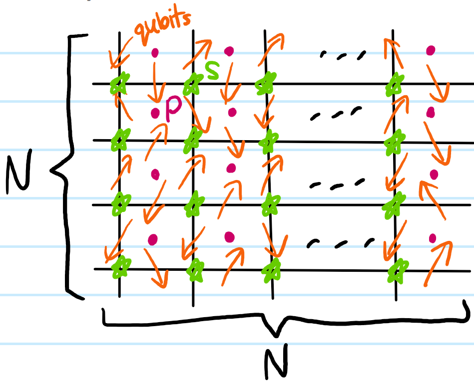
To begin, consider an \(N\times N\) square lattice \(\Lambda\) with a qubit placed at each edge as follows:
The vertices of the lattice \(\Lambda\) are called stars \(S\) while its faces are called plaquettes \(P\) (which can also be viewed as the vertices of the dual lattice \(\Lambda^*\), etc.). Since \(\Lambda\) is an \(N\times N\) square lattice, one might initially think that there are \(2N(N+1)\) qubits; however the catch is that opposite ends of the lattice are identified with each other, so that there are in fact only \(2N^2\) qubits. More importantly, this imposition of periodic boundary conditions endows \(\Lambda\cong S^1\times S^1\) with the topology of a torus, hence the name “toric code”.
A priori, the state space \(\mathcal H\) of \(2N^2\) qubits has dimension \(\text{dim}\mathcal H=2^{2N^2}\) (though if some/all of these qubits are identical then it may be less than this). Using the notation \(\sigma_i^x\) as a shorthand for the operator \(1_1\otimes…\otimes 1_{i-1}\otimes\sigma^x\otimes 1_{i+1}\otimes…\otimes 1_{2N^2}\) acting on \(\mathcal H\) and similarly for \(\sigma_i^y\) and \(\sigma_i^z\), one can define star and plaquette four-body interaction operators \(A_S,B_P\) associated respectively to stars \(S\) or plaquettes \(P\) in \(\Lambda\) by:
\[A_S:=\prod_{i\in S}\sigma_i^z\]
\[B_P:=\prod_{i\in P}\sigma_i^x\]
where the notation “\(i\in S\)” denotes the set of \(4\) qubits nearest to a given star \(S\), and similarly for “\(i\in P\)”; the notation \(\prod_{i\in S}\) or \(\prod_{i\in P}\) does not suffer from any operator ordering ambiguity because Pauli operators on distinct qubits (regardless of their \(x,y,z\) nature) trivially commute.
For any two stars \(S,S’\), and any two plaquettes \(P,P’\), one can check (without any motivation yet at this point) that:
\[[A_S,A_{S’}]=[B_{P},B_{P’}]=[A_S,B_P]=0\]
Specifically, if the stars or plaquettes are well-separated from each other then these are always trivially true so it suffices to just check the “edge cases” so to speak when the stars or plaquettes are close enough to share qubits. Then, for each such shared qubit, one just has to apply the anticommutation relation \(\{\sigma^{\alpha},\sigma^{\beta}\}=2\delta^{\alpha\beta}1\). Notably, the commutation relation \([A_S,B_P]=0\) relies on the fundamental fact that a star \(S\) and plaquette \(P\) which are adjacent to each other always share only \(2\) qubits, and \(2\) is even so \((-1)^2=1\).
Finally, suppose one thinks of the lattice of qubits as a spin lattice such that the spins interact via the following Hamiltonian:
From the above discussion, it follows that for any star \(S\) or plaquette \(P\), one has:
\[[H,A_S]=[H,B_P]=0\]
There are \(N^2\) stars and \(N^2\) plaquettes, so this would suggest that one is free to specify the however, using a “Stokes theorem” type of argument (basically a more refined version of earlier arguments for showing \([A_S,A_{S’}]=[B_P,B_{P’}]=0\)), one can convince oneself inductively (i.e. playing around with small \(N=1,2,…\) etc.) that it is precisely thanks to the toric topology of \(\Lambda\) that one has the constraints:
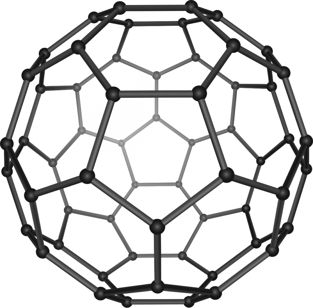
The purpose of this post is to explain why, experimentally, one only observes \(4\) electric dipole transitions in the IR spectrum of buckminsterfullerene, also known as \(\text C_{60}\) or informally as the buckyball:
Buckyball Basics
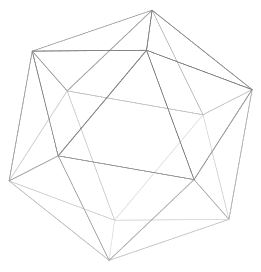
The simplest conceptual way to construct a buckyball is to start with a regular icosahedron:
which has \(F=20\) equilateral triangular faces, \(V=12\) vertices, and \(E=30\) edges; notice this obeys Euler’s formula \(F+V=E+2\). Then, by simply “shaving off” each of the \(V=12\) vertices; it is clear from the picture these \(12\) vertices would transform into \(12\) pentagonal faces, each surrounded by \(5\) hexagonal faces so that no \(2\) pentagonal faces share an adjacent edge, yielding a buckyball topology (and geometrically, all \(\text C-\text C\) covalent bonds should be of equal length). This shaving process increases the number of faces to \(F’=32\) (of which \(12\) are pentagonal and \(20\) are hexagonal), the number of vertices to \(V’=60\) (i.e. just the number of carbon atoms), and the number of edges to \(E’=90\) such that Euler’s formula is maintained \(F’+V’=E’+2\).
IR Spectroscopy Selection Rules
Recall that within the Born-Oppenheimer approximation, the \(N\) nuclei of some molecule are “clamped” at positions \(\textbf X:=(\textbf X_1,…,\textbf X_N)\) and are regarded as moving in the effective potential \(V_{\text{eff}}(\textbf X)\) due to the electrons \(e^-\), so that the molecular Hamiltonian is:
\[H=T_{\text n}+V_{\text{eff}}(\textbf X)\]
If in addition one approximates \(V_{\text{eff}}(\textbf X)\) by a harmonic potential about the (stable) equilibrium configuration \(\textbf X_0\) of the nuclei:
then, upon diagonalizing the Hessian \(\left(\frac{\partial^2 V_{\text{eff}}}{\partial\textbf X^2}\right)_{\textbf X_0}\) into the orthonormal eigenbasis of its normal modes, one obtains \(3N\) decoupled simple harmonic oscillators so the spectrum of \(H\) is just that of an anisotropic harmonic oscillator in \(\textbf R^{3N}\), at least within all the assumptions made so far (e.g. ignoring anharmonicity of \(V_{\text{eff}}(\textbf X)\)). Each Fock eigenstate \(|n_1,n_2,…,n_{3N}\rangle\) of \(H\) (thought of as a vibrational eigenstate because one can view \(H\) as a Hamiltonian governing vibrations/SHM of the nuclei about equilibrium) is thus a product \(|n_1,n_2,…,n_{3N}\rangle=\otimes_{i=1}^{3N}|n_i\rangle\) of suitable \(1\)D quantum harmonic oscillator wavefunctions.
IR radiation is just like any other electromagnetic radiation in that (within the dipole approximation, which is fair for long-wavelength IR radiation despite the larger size of molecules) it stimulates electric dipole transitions via the time-dependent perturbation \(\Delta H=\Delta H(t)\) to the molecular Hamiltonian \(H\):
and the molecule is assumed to be neutral \(\sum_{\text{nuclei }i}Z_i=\sum_{\text{electrons }i}\). By Fermi’s golden rule, the molecular transition rate between two distinct vibrational \(H\)-eigenstates \(|n_1,…,n_{3N}\rangle\to|n’_1,…,n’_{3N}\rangle\) is proportional to the mod-square of the matrix element of the (time-independent amplitude of the) perturbation:
However, most IR spectroscopy experiments (e.g. IR laser sources in FTIR spectrometers) use unpolarized IR radiation, so this means one should really replace by an isotropic averaging factor of \(1/3\) and forget about (as far as selection rules are concerned) a factor of \(|\textbf E_0|^2\), so just focus on:
Similar to what was done earlier for the effective potential \(V_{\text{eff}}(\textbf X)\), one can also Taylor expand the dipole moment operator \(\boldsymbol{\pi}\) withinthe configuration space \(\textbf X\) of the nuclei about the equilibrium configuration \(\textbf X_0\):
Sandwiching this in the matrix element, the constant term \(\boldsymbol{\pi}(\textbf X_0)\) (which represents the possibility of a permanent electric dipole like in a water molecule) vanishes by orthogonality of the distinct vibrational \(H\)-eigenstates, so the quantity of interest is just:
This immediately leads to a “gross selection rule” for two vibrational \(H\)-eigenstates to be coupled by the IR perturbation \(\Delta H\), namely that the Jacobian \(\left(\frac{\partial\boldsymbol{\pi}}{\partial\textbf X}\right)_{\textbf X_0}\) must be non-vanishing; physically, this means that only the normal modes of the nuclear vibration that experience a change in \(\boldsymbol{\pi}\) when the nuclei are slightly displaced from \(\textbf X_0\) will be IR-active.
…main point of this section is to explain that IR transitions are low-energy excitations require a change in electric dipole moment b/w initial and final states, which, factoring out the charge e, means the matrix element of the position observable b/w two states must be non-zero by Fermi’s golden rule. There are actually \(2\) selection rules for IR spectroscopy; the gross selection rule is that \(\partial\boldsymbol{\pi}/\partial\) must be zero.
Character Tables of Finite Group Representations
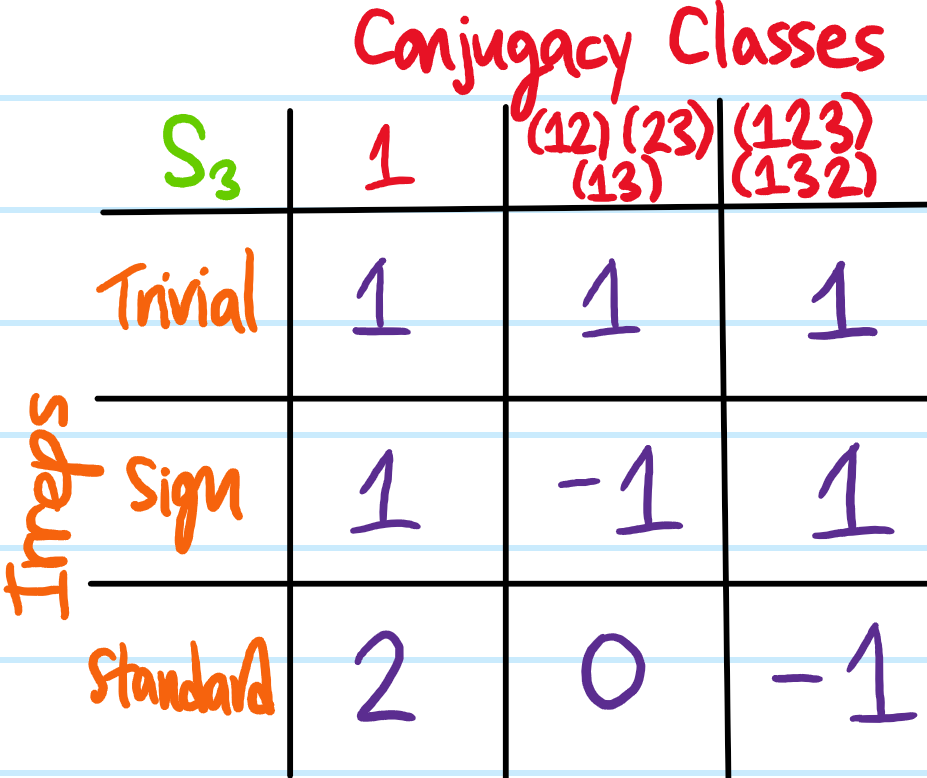
As a warmup, consider the symmetric group \(S_3=\{1, (12), (13), (23), (123), (132)\}\) of order \(|S_3|=3!=6\). Then \(S_3\) can be partitioned into \(3\) conjugacy classes, namely \(S_3=\{1\}\cup\{(12), (13), (23)\}\cup\{(123), (132)\}\). Each \(S_3\) conjugacy class maps onto an \(S_3\)-irrep, so there will also be three \(S_3\)-irreps. One of them is always just the trivial irrep whereby the permutations do nothing to all vectors. For symmetric groups, there is also always the sign irrep \(1,(123),(132)\mapsto 1\) and \((12),(13),(23)\mapsto -1\) such that odd permutations do nothing to all vectors but even \(A_3\)-permutations flip vectors across the origin. Finally, there is the standard \(S_3\)-irrep that one might intuitively think about as acting on the vertices of an equilateral triangle which rigidly drags the whole Cartesian plane \(\textbf R^2\) along with it. Note the dimensions of these \(S_3\)-irreps are the only ones that could have been compatible with its order \(6=1^2+1^2+2^2\).
Each \(S_3\)-irrep is associated with its own character class function which can be evaluated on an arbitrary representative of each conjugacy class. For instance, the trivial irrep is \(1\)-dimensional and its character always evaluates to \(1\) on all conjugacy classes. The sign irrep is also \(1\)-dimensional but its character evaluated on each conjugacy class is instead the sign of the permutations in that conjugacy class. Finally, noting that \(\cos(2\pi/3)=-1/2\) and that the trace of a rotation in \(\textbf R^2\) by angle \(\theta\) is \(2\cos\theta\), the following character table for \(S_3\) may be obtained:
So far this example has been fairly abstract. To bridge this “abstract nonsense” with chemistry, consider the specific example of the ammonia molecule \(\text{NH}_3\):
In this case, rather than pulling a random group (like \(S_3\)) out of thin air, here one can use the ammonia molecule to motivate studying the specific group of actions on \(\textbf R^3\) that leave it looking like nothing happened. In chemist jargon, one is interested in the point group of the ammonia molecule, the adjective “point” implying that any such action on \(\textbf R^3\) must have at least one fixed point in space (commonly chosen to be the origin) so that e.g. translations of the ammonia molecule are disregarded (cf. the distinction in special relativity between the Poincare group and its Lorentz subgroup). Note that this is indeed a group thanks to its very definition (if one action leaves ammonia looking like nothing happened, and a second action also leaves ammonia looking like nothing happened, then composing them will also leave ammonia looking like nothing happened).
So what is the point group of the ammonia molecule? For this, there isn’t really any super rigorous/systematic way to do it, one just has to stare hard at the molecule and think…
Clearly, one way to leave ammonia looking like nothing happened is to literally do nothing. There is also manifestly \(C_3\) rotational symmetry (by \(120^{\circ}\) or \(240^{\circ}\)). Finally, there are \(3\) reflection symmetries about “vertical” mirror planes. As a mathematician, it is thus easy to recognize that the point group of the ammonia molecule is just the dihedral group \(D_3\) (which happens to be isomorphic to \(S_3\)). However, as a chemist one would instead refer to this as the “\(C_{3v}\) point group”, where the \(C\) and the \(3\) subscript are meant to emphasize the \(C_3\) subgroup of rotational symmetries mentioned above, while the “\(v\)” subscript is meant to emphasize that the mirror planes are “vertical”. Strictly speaking, one should also check that there are no horizontal mirror planes, inversion centers, or improper rotation axes in order to be able to confidently assert that the point group of ammonia really is \(C_{3v}\) rather than \(C_{3v}\) merely being a subgroup of an actually larger point group.
The isomorphism \(C_{3v}\cong D_3\cong S_3\) means that by happy chance the character table for the ammonia point group \(C_{3v}\) is already known. For instance, the transpositions \((12),(23),(13)\) in \(S_3\) map onto vertical mirror plane reflections in \(C_{3v}\), while the \(3\)-cycles \((123),(132)\) are simply \(C_3\) rotations. Indeed, the \(3\)-dimensional \(C_{3v}\)-representation on the ammonia molecule itself embedded rigidly in \(\textbf R^3\) is reducible into a direct sum of the trivial irrep acting on the \(1\)-dimensional \(z\)-axis and the standard irrep acting on the \(2\)-dimensional \(xy\)-plane. It is also worth verifying that the columns of the character table satisfy orthonormality \(\sum_{\text{ccl}\text{ of }C_{3v}}|\text{ccl}|\chi_{\phi}(\text{ccl})\chi_{\phi’}(\text{ccl})=|C_{3v}|\delta_{\phi\cong\phi’}\) for any \(2\) \(C_{3v}\)-irreps \(\phi,\phi’\).
One can also consider how various scalar-valued and vector-valued polynomials on \(\textbf R^3\) transform passively under the \(C_{3v}\) point group. For instance, any function \(f=f(\rho)\) of the cylindrical coordinate \(\rho:=\sqrt{x^2+y^2}\) only, such as \(f(\rho)=\rho^2\), will transform under the trivial \(C_{3v}\)-irrep.
Making the reasonable assumption that all \(60\) carbon atoms are specifically of the \(^{12}\text C\) isotope, and are therefore identical bosons, so something about the permutation group \(S_{60}\)? (formalize the earlier comment about “looking the same” via the idea of identical quantum particles/ bosons and fermions where in that case the vectors are not in \(\textbf R^3\) but state vectors in the symmetrized tensor product Hilbert space of identical bosons)
The purpose of this post is to explain several techniques for laser cooling and laser trapping of atoms. In order to better emphasize key conceptual points, it will take the approach of posing problems, followed immediately by their solutions.
Problem #\(1\): Recall that any locally conserved field is associated to a continuity equation \(\dot{\rho}+\partial_{\textbf x}\cdot\textbf J=0\). In particular, the local flow of the corresponding conserved quantity can always be interpreted in terms of a velocity field \(\textbf v\) (with SI units of meters/second) by enforcing that \(\textbf J=\rho\textbf v\). Interpret this in the context of fluid mechanics and electromagnetism.
Solution #\(1\): In fluid mechanics, mass is locally conserved, so \(\rho\) could represent mass density while \(\textbf J\) represents mass flux. Momentum is also locally conserved provided there are no external body forces acting on the fluid, so in that case \(\rho\) would be a vector field representing momentum density while \(\textbf J\) would be the stress tensor field representing momentum transport (this is just the Navier-Stokes equations). Similar comments can be made about energy, angular momentum, etc.
In electromagnetism, electric charge is locally conserved, so in that case \(\rho\) represents charge density while \(\textbf J\) represents an electric current. Similarly, the total energy stored in both electromagnetic fields and electric charges is locally conserved. In that case, the continuity equation in linear dielectrics takes the form:
where the electromagnetic field energy density is \(\mathcal E:=(\textbf D\cdot\textbf E+\textbf H\cdot\textbf B)/2\) and the Poynting vector \(\textbf S:=\textbf E\times\textbf H\). If an electromagnetic wave propagates with group velocity \(|\textbf v|\leq c\) in some linear dielectric, it follows that \(\textbf S=\mathcal E\textbf v\) (similar comments apply to momentum density; indeed they are unified in the Maxwell stress tensor).
Problem #\(2\): Within the framework of classical electromagnetism, what is the formula for the radiation pressure \(p_{\gamma}\) exerted at normal incidence to an absorbing surface \(\hat{\textbf n}\) with reflection coefficient \(R\)?
Solution #\(2\): Just as \(\textbf S=\mathcal E\textbf v\) (from Solution #\(1\)), so the radiation pressure is a certain projection of an isotropic current for the momentum density \(\boldsymbol{\mathcal P}\):
The photon dispersion relation \(\mathcal E=|\boldsymbol{\mathcal P}||\textbf v|\) in a linear dielectric then implies that the radiation pressure \(p_{\gamma}=(1+R)\mathcal E\cos^2\theta\) is given by a Malusian proportionality with the energy density stored in the EM field (aside: how is this related to the equation of state \(p=\mathcal E/3\) for a photon gas?).
Problem #\(3\): An atom moving at (nonrelativistic) speed \(v\) (in the lab frame) and meets a counter-propagating laser beam of incident intensity \(I\) and frequency \(\omega\) (both in the lab frame, where of course it is assumed that the laser source is also at rest in the lab frame). Estimate the velocity-dependent scattering force \(F_{\gamma}(v)\) exerted on the atom and its maximum possible value \(F_{\gamma}^*> F_{\gamma}(v)\).
Solution #\(3\): Heuristically, the scattering force might also be called the radiation force as it’s roughly just the radiation pressure \(p_{\gamma}\) exerted on the cross-section \(\sigma(\omega_D)\) of the atom (evaluated at the Doppler-shifted frequency \(\omega_D:=\omega\sqrt{(1+\beta)/(1-\beta)}\approx \omega+kv\)):
where in the last expression it is assumed that the Doppler detuning \(\delta_D=\omega_D-\omega_{01}\) is small so in particular both \(I\) and \(\sigma_{01}\) are taken to be independent of \(\omega_D\). This is from the perspective of stimulated absorption. On the other hand, because all the analysis is implicitly in the steady state, one can also view this from the perspective of spontaneous emission:
Note that these two formulas for \(F_{\gamma}(v)\) are not exactly equal, but approximately so at low irradiance \(s\ll 1\) (how to rationalize why?). Meanwhile, on resonance \(\delta_D=0\), in the high-irradiance \(s\to\infty\) limit, the theoretical max scattering force achievable is \(F_{\gamma}^*=\hbar k\Gamma/2\).
Problem #\(4\): Atoms flying out of an oven at temperature \(T\) are collimated to form an atomic beam which meets a counterpropagating laser \(s,\omega\). Without any frequency compensation on the laser \(\omega\), show how to determine the terminal velocity \(v_{\infty}\) of the atoms.
Solution #\(4\): The idea is that when one is far detuned from \(\omega_D\), there is hardly any scattering force and so the atoms move at roughly constant velocity. It is only in a small window \(\omega_D\in[\omega_{01}-\Gamma/2,\omega_{01}+\Gamma/2]\) that there is any significant scattering force. In this near-resonance regime, one can therefore set up an equation of motion \(M\dot v=-F_{\gamma}(v)\) whose solution is:
where the initial speed can be taken as the most probable one \(v_0=\sqrt{2k_BT/M}\), and the time \(\Delta t\) can be estimated by considering the situation where \(\omega+kv_0=\omega_{01}+\Gamma/2\) and \(\omega+kv_{\infty}=\omega_{01}-\Gamma/2\) (actually not sure about this).
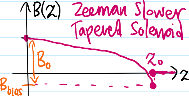
Problem #\(5\): If the atomic beam emerging from the oven along with the counterpropagating laser are oriented along some “\(z\)-axis”, write down the magnetic field \(\mathbf B(z)=B(z)\hat{\textbf k}\) required to make a Zeeman slower.
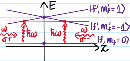
Solution #\(5\): Assuming one is working at relatively low magnetic field strengths, the low-field basis which diagonalizes the perturbative hyperfine Hamiltonian \(\Delta H_{\text{HFS}}\propto\textbf I\cdot\mathbf J\) is \(|f,m_f\rangle\). In this basis, the expectation of the perturbative Zeeman Hamiltonian \(\Delta H_{\text{Zeeman}}\) is approximately:
Thus, if one is exploiting an electric dipole transition from a “ground state” \(|fm_f\rangle\) to an “excited state” \(|f’m’_f\rangle\), then one requires the difference in the Zeeman shifts experienced by these \(2\) levels to precisely compensate for the Doppler detuning \(\delta_D=\omega+kv-\omega_{01}\):
In practice, one would like to achieve a constant deceleration \(a>0\) so that \(v^2=v_0^2-2az\). This requires a magnetic field from e.g. a tapered solenoid of the form:
where \(z_0:=v_0^2/2a\) is the stopping distance, \(B_0:=\frac{\hbar kv_0}{\mu_B(g_{f’}m’_f-g_fm_f)}\) can be interpreted as \(B_0=B(0)-B(z_0)\), and the bias field is \(B_{\text{bias}}=\frac{\hbar(\omega-\omega_{01})}{\mu_B(g_{f’}m’_f-g_fm_f)}\); or at least, if one wishes to completely stop the atoms at \(z=z_0\) (if not, then one may need to experimentally lower \(B_{\text{bias}}\) until one obtains a desired terminal velocity; in that case one should then discontinuously turn off the magnetic field \(B(z):=0\) for \(z>z_0\) so that the E\(1\) transition would again be substantially detuned from resonance and so experience a negligible scattering force \(F_{\gamma}\) after the atoms exit the Zeeman slower).
Problem #\(6\): For the specific case of say sodium atoms \(\text{Na}\) (analogous remarks apply to any alkali atom), explain why electric dipole transitions between the stretched states \(|fm_f\rangle=|22\rangle\) in \(3s_{1/2}\) and \(|f’m’_f\rangle=|33\rangle\) in \(3p_{3/2}\) are a good choice for laser cooling via the scattering force \(F_{\gamma}\)? In this case, what should be the corresponding value of \(B_0\) used in a Zeeman slower (the transition has \(\lambda_{01}=589\text{ nm}\))? What should be the polarization of the incident laser light?
Solution #\(6\): This E\(1\) transition is not only allowed but also forms a closed cycle thanks to the usual E\(1\) selection rules, ensuring no optical pumping into dark states that would prevent a given atom from experiencing any further scattering. One can check that \(B_0\approx 0.12\text{ T}=1200\text{ G}\) is reasonable to achieve in the lab. The incident photons should be \(\sigma^+\) circularly-polarized along the quantization axis \(\hat{\textbf k}\) defined by the \(\textbf B\)-field along which the atomic beam is also propagating.
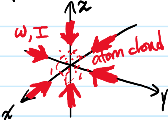
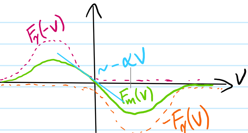
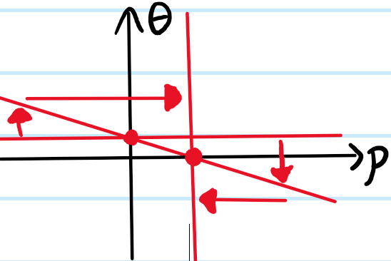
Problem #\(7\): Show, stating any assumptions made, that the velocity-dependent optical molasses force \(F_m(v)\approx -\alpha v\) along an arbitrary axis looks like linear damping with some damping coefficient \(\alpha>0\) for an appropriately-chosen laser detuning \(\delta\). Hence, show that the atom’s kinetic energy \(T(t)=T(0)e^{-t/\tau}\) (supposedly) decays exponentially with time constant \(\tau=m/2\alpha\).
Solution #\(7\): Along any of the \(3\) Cartesian axies, the component of the optical molasses force \(F_m(v)\) along that axis is a superposition of two opposite (but not necessarily equal) scattering forces:
So in order for \(\alpha>0\) to actually be damping, one requires \(\delta<0\) to be red-detuned as suggested in the picture. It turns out that in order to treat the two laser beams independently (as has been implicitly done above), they both have the same low \(s\ll 1\) so that neither one saturates the E\(1\) transition too much. In this simple model of optical molasses, one should therefore really take:
In some sense, the fact that it looks like linear damping near \(v=0\) is not really conceptually any different from the fact that e.g. systems looks like simple harmonic oscillators near stable equilibria; it’s just taking the \(1\)-st order term in a Taylor series in \(v\).
Kinetic energy is lost through the dissipative power of the molasses force:
where \(\tau=m/2\alpha\) is usually on the order of microseconds. This suggests that there is no cooling limit, i.e. that one can quickly cool down arbitrarily close to \(T\to 0\), but this turns out to be impossible, see Problem #\(9\).
Problem #\(8\): For a random walk \(\textbf X_1,\textbf X_2,…,\textbf X_N\) of \(N\) steps, each of identical length \(L=|\textbf X_1|=|\textbf X_2|=…=|\textbf X_N|\), what is the expectation of the total displacement squared \(\langle|\textbf X_1+\textbf X_2+…+\textbf X_N|^2\rangle\)?
Problem #\(9\): Conceptually, what is the issue with the approach taken in Solution #\(7\)? Upon amending it, show that there is actually a Doppler cooling limit, namely a minimum temperature \(T_D\) that can be achieved using the optical molasses technique, given by:
\[k_BT_D=\frac{\hbar\Gamma}{2}\]
Solution #\(9\): The issue with Solution #\(7\) is that, while it accounts for the momentum kick given to the atom during stimulated absorption of photons and also recognizes that spontaneous emission averages to no momentum kick, it neglects fluctuations in both the number of photons absorbed and in the number of photons scattered. Using the result of Problem #\(8\), except here conceptually it’s not a random walk in real space but rather in momentum space with \(\langle p_z^2\rangle(t)=2(\hbar k)^2(2\gamma)t\), the kinetic energy \(T_z\) of an atom in the optical molasses now evolves as (see Foote textbook for the detailed arguments, some sketchy assumptions involved too, and turns out ultimately wrong, see Problem #\(10\)):
is minimized for red-detuned \(\delta<0\) at \(2\delta/\Gamma=-1\), yielding the Doppler cooling limit \(k_BT_D=\hbar\Gamma/2\) as claimed.
Problem #\(10\): Explain why, even after accounting for Poissonian fluctuations in the stimulated absorption and spontaneous emission of photons, the Doppler cooling limit for the optical molasses technique above rests on a “spherical cows in vacuum” foundation.
Solution #\(10\): Simply put, the assumption of a \(2\)-level atom has been implicitly lurking in the discussion the whole time, but it turns out that if one leverages the existence of other sublevels, one can do even better than the Doppler cooling limit above would suggest. Note also that the optical molasses laser cooling technique only provides confinement in \(\textbf k\)-space, but not so much in \(\textbf x\)-space which is also relevant; in other words, laser trapping is to \(\textbf x\) what laser cooling is to \(\textbf k\).
Problem #\(11\): In light of Problem #\(10\), draw \(3\) pictures that summarize how a magneto-optical trap (MOT) works. In particular, it should be clear that the MOT could not work with just a \(2\)-level atom. Also write down explicitly a formula for the MOT force \(F_{\text{MOT}}(z,v)\).
Solution #\(11\):
The MOT force \(F_{\text{MOT}}(z,v)\) is conceptually identical to the optical molasses force \(F_m(v)\) only now the detuning includes not only the \(v\)-dependent Doppler shift but also the \(z\)-dependent Zeeman shift (more precisely, the formula \(F_{\text{MOT}}(z,v)\) that will be given below is the component of the net MOT force \(\textbf F_{\text{MOT}}(\textbf x,\textbf v)\) along the quantization \(z\)-axis of the quadrupolar anti-Helmholtz MOT \(\textbf B\)-field near the origin \(\textbf x\approx\textbf 0\) whose purpose is to generate a nearly uniform magnetic field gradient; a similar equation holds in the \(\rho\)-direction except one should note from \(\frac{\partial}{\partial\textbf x}\cdot\textbf B=0\) that \(\frac{\partial B_{\rho}}{\partial\rho}=-\frac{1}{2}\frac{\partial B_z}{\partial z}\)).
Making the same low Doppler shift assumption \(kv\ll\Gamma\) but now also a low Zeeman shift assumption \(\frac{g’_f\mu_B}{\hbar}\frac{\partial B_z}{\partial z}z\ll\Gamma\), one can check that this reduces to the previous linear damping force of the optical molasses together with a Hookean spring force:
\[F_{\text{MOT}}(z,v)=-\alpha v-\beta z\]
where the spring constant is \(\beta=\frac{\alpha g’_f\mu_B}{\hbar k}\frac{\partial B_z}{\partial z}\) and the damping coefficient \(\alpha\) is as before in Problem #\(7\). Usually, the atom will be overdamped (as is desirable) \(\alpha^2>4\beta m\).
Problem #\(12\): State one advantage and one disadvantage of a MOT compared with just the optical molasses technique.
Solution #\(12\): The advantage of a MOT is that its capture velocity \(v_{c,\text{MOT}}\gg v_{c,m}\) is much greater than that of optical molasses so it is a better trapper, hence its name (indeed, one can load a MOT simply by firing a room-\(T\) vapor, or to get more atoms one can first Zeeman slow them). The disadvantage is that it is not as good of a laser cooler; optical molasses is able to reach much colder temperatures, surpassing the naive Doppler cooling limit \(k_BT_D=\hbar\Gamma/2\) mentioned earlier (this is because of various sub-Doppler cooling mechanisms, notably Sisyphus cooling, that are elaborated upon in the next problem; all that matters for now is that such sub-Doppler cooling mechanisms are effectively disabled when the Zeeman shift exceeds the light shift as in a MOT).
Problem #\(13\): In a MOT, where does the trapping come from?
Solution #\(13\): It does not come from the quadrupolar \(\textbf B\)-field, but rather
Problem #\(14\): Draw a picture to explain how Sisyphus cooling allows. What is the new cooling limit?
Problem #\(15\): Show that the magnetic field strength \(|\textbf B(\textbf x)|\) in free space can never have a strict local maximum provided \(\dot{\textbf E}=\textbf 0\) (this is one version of Earnshaw’s theorem).
But thanks to the assumptions of the problem the term on the left vanishes, and in addition to the absence of magnetic monopoles, one concludes that \(\left|\frac{\partial}{\partial\textbf x}\right|^2\textbf B=\textbf 0\).
Now, \(|\textbf B(\textbf x)|\) satisfies the claim if and only if \(|\textbf B(\textbf x)|^2\) satisfies it. In turn, one just has to check that the Hessian \(\frac{\partial^2|\textbf B|^2}{\partial\textbf x^2}\) does not have \(3\) negative eigenvalues anywhere. A sufficient (but not necessary) condition for this would be if \(\text{Tr}\frac{\partial^2|\textbf B|^2}{\partial\textbf x^2}\geq 0\) everywhere. But the trace of the Hessian is just the Laplacian of the original scalar field:
Problem #\(16\): What is the high-level mechanism of magnetic trapping? What are the \(3\) most common kinds of magnetic traps? (just draw a picture of each one with some annotations, no need for long explanations)
Solution #\(16\): Just as in the Stern-Gerlach experiment, magnetic dipoles in non-uniform magnetic fields experience a force that pushes them towards weaker or stronger magnetic field depending on their orientation relative to the magnetic field. The difference is that in the Stern-Gerlach experiment the atoms are flying in at hundreds of meters/second and getting deflected, way beyond capture velocity, whereas in magnetic trapping they have already been laser cooled. The diThe \(3\) most common magnetic traps are the quadrupole trap (made from a pair of anti-Helmholtz coils as in a MOT), a time-averaged orbiting potential (TOP)trap, and an Ioffe-Pritchard trap, the last of which is the most common and simply consists of \(4\) long cylindrical bars (which form a “linear quadrupole” in direct analogy with an electrostatic quadrupole) and \(2\) Helmholtz-like coils. Key words: radial/\(\rho\)-trapping and axial/\(z\)-trapping. Due to the result of Problem #\(14\), it follows that one can only trap atoms in low-field seeking states (such atoms are called low-field seekers).
Good overview here: https://arxiv.org/pdf/1310.6054
The purpose of this post is to review the theory behind several standard amplitude-splitting interferometers.
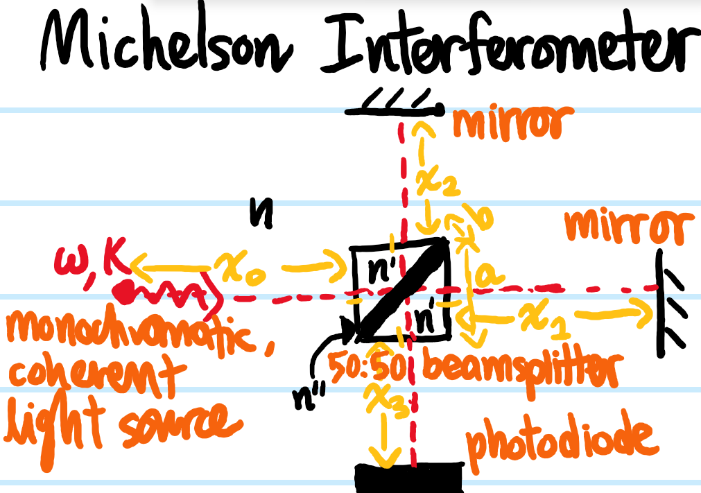
Michelson Interferometer
The simplest possible version of a Michelson interferometer is the following:
For now, consider for simplicity a monochromatic light source of frequency \(\omega=ck=nvk=n’v’k=n^{\prime\prime}v^{\prime\prime}k\). In “chronological order”, the phases accrued by \(2\) amplitude-split reflected and transmitted rays in their respective journeys from the light source to the photodiode are explicitly:
where it has been assumed that \(n'<n^{\prime\prime}\) and that \(n<n_{\text{mirrors}}\), though as far as their relative phase difference \(\Delta\phi\) is concerned, because \(\textbf R\) is an additive abelian group it will always just be:
\[\Delta\phi=|\phi_2-\phi_1|=2nk\Delta x\]
where the arm-length difference is \(\Delta x:=|x_2-x_1|\) (to get a \(50:50\) beam splitter there should also be some constraint on \(a,b,n,n’,n^{\prime\prime}\) coming from the Fresnel equations). If the photodiode has sampling period \(T_s>0\), then one expects that the signal it measures will be a time-averaged irradiance of the form (it is being assumed here that the beam splitter really is exactly \(50:50\)):
where \(\cos\Delta\phi\) is the interference term which is sensitive to the relative phase difference\(\Delta\phi\) between the two interfering waves of identical frequency \(\omega\).
On the other hand then, given two distinct frequencies \(\omega<\omega’\) separated by \(\Delta\omega:=\omega’-\omega>0\), one can repeat the story above, this time measuring an irradiance:
is only non-negligible in the limit \(\Delta\omega T_s\ll 1\) which is typically not satisfied, and so here is taken to vanish. The key takeaway from this is that, while any two waves will interfere, waves of distinct frequencies \(\omega’\neq\omega\) do not in general interfere in an easy-to-measure way, i.e. only interference between waves of the same frequency \(\omega\) tends to be measurable.
That being said, it is essential to stress that interference between waves of the same \(\omega\) is interference nonetheless, and the resultant interference pattern \(I(\Delta\phi,\Delta\phi’)\) is readily measured in experiments and still extremely useful. One example of this is in the case where \(\Delta\omega\) is small, such as between \(2\) atomic fine or hyperfine transitions. Then the interference pattern can be written as a function of the Michelson interferometer arm-length difference \(\Delta x\):
This is analogous to the phenomenon of beats in the \(t\)-domain; here in a spatial domain \(\Delta x\), the low-frequency envelope \(\cos n(k’-k)\Delta x\) is modulated by high-frequency fringes \(\cos n(k+k’)\Delta x\). By finding a \(\Delta x=\Delta x_0\) where fringes disappear due to vanishing of the envelope \(\Delta k:=k’-k=\pi/2n\Delta x_0\), one can thereby obtain the frequency difference \(\Delta\omega=nv\Delta k\) assuming \(n\) is non-dispersive. The envelope is sometimes phrased in terms of the fringe visibility:
As its name suggests, when the fringes become invisible (i.e. fringe visibility becomes \(V(\Delta x_0)=0\)), then one again recovers the same frequency difference \(\Delta\omega\) as above.
Another point implicitly assumed above and worth stressing is that the relative phase difference \(\Delta\phi\) of the two interfering waves have to maintain temporal coherence \(\frac{\partial\Delta\phi}{dt}=0\) at the photodiode position.
More generally, assuming that waves of any two distinct frequencies, no matter how close, do not interfere, a highly polychromatic signal containing irradiance \(2\hat I(k)dk\) in the wavenumber interval \([k,k+dk]\) would be expected to exhibit a Michelson interference pattern of the form:
Or equivalently, because \(\hat I(\Delta x)\in\textbf R\) is expected to be real-valued for all \(\Delta x\), it follows that its Fourier transform \(\hat I(k)\) needs to be Hermitian \(\hat I(-k)=\hat I^{\dagger}(k)\). This means one can rewrite this as an inverse Fourier transform:
and is the basis of the Fourier transform infrared spectrometer(FTIR) where a Michelson interferometer is employed along with one mirror on a motorized translation stage to vary \(\Delta x\) and a photodiode to measure the corresponding total interference pattern \(I(\Delta x)\) from all the wavenumbers \(k\in(0,\infty)\).
Note in all of the above discussion it has been implicitly assumed that all the beams in the Michelson interferometer are perfectly collimated, etc. so that the photodiode observes an interference pattern \(I(\Delta x)\) which would vary with arm-length difference \(\Delta x\) but spatially across the photodiode surface would be uniform; in practice, due to misalignment (accidental or deliberate) or imperfect collimation because the light source is not a point but extended, etc. there is not only an interference pattern in \(\Delta x\)-space, but in real space \((x,y)\) across the photodiode surface too; this whole interference profile \(I(x,y,\Delta x)\) would then change as \(\Delta x\) were to evolve (this is best understood by putting one’s eye at the photodiode location and looking into the beam splitter; one would then see \(2\) virtual images of the light source behind a mirror sitting around \(\sim 2 x_2\) away, separated by \(\sim 2\Delta x\). Conceptually, one can then just forget about the whole Michelson interferometer setup and pretend as if one just had \(2\) coherent light sources interfering with each other on a distant screen. Using this perspective, it is clear that the spatial fringes one observes will be sections of hyperbolae.
Finally, it is worth mentioning that sometimes a minor variant of the Michelson interferometer (called a Twyman-Green interferometer) is used for better collimation of the incident light beam. In addition, if instead of a beam splitter one were to use a half-silvered mirror, then a compensator may also need to be added (this would compensate not only for the optical path length difference in monochromatic incident light but also for optical dispersion in the case of polychromatic incident light).
Mach-Zehnder Interferometer
The setup is the following:
Kinda similar to Michelson except light never retravels its path.
Also, instead of a single photodiode on which equal-frequency waves interfere, have two photodiodes to measure the intensities on each output port of the last beamsplitter.
Idea is that for a \(50:50\) beamsplitter, a unitary (probability-conserving) to describe action on photon probability amplitudes for going down each arm of the Mach-Zehnder.
Fabry-Perot Interferometer
Miscellaneous: Thin Film Interferometer, Haidinger Fringes & Newton’s Rings
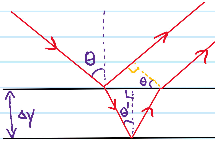
Problem: Write down the conditions for maximum constructive and destructive interference in a thin-film interferometer.
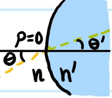
Solution: For a light wave incident at angle \(\theta\):
This is the phase shift between the amplitude-split waves arising solely from their path length difference and the magnitude of the impedance mismatch between the \(2\) dielectrics. However, depending on the sign of this impedance mismatch (i.e. whether \(k>k’\) or \(k<k’\)), one of the waves will, at one of the reflections, also accrue an additional \(\pi\) phase shift. So the total phase shift is actually:
\[\Delta\phi=2k_y’\Delta y+\pi\]
and from this the condition for maximum constructive interference \(\Delta\phi=2\pi m\) or maximum destructive interference \(\Delta\phi=2\pi m+\pi\) can be written. To actually compute the resultant light wave’s electric and magnetic fields, one would have to use the Fresnel equations, separately looking at \(s\) and \(p\)-polarized light.
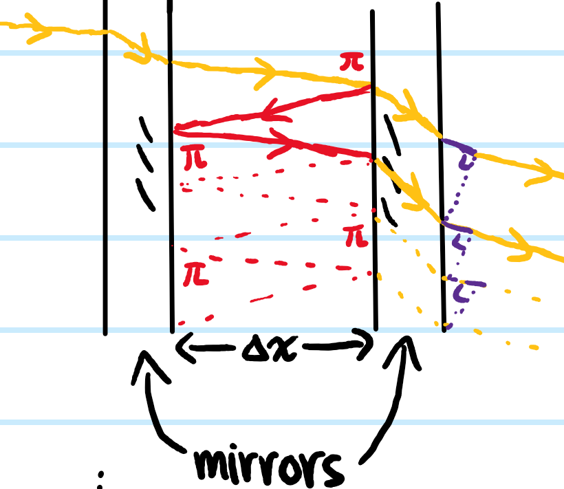
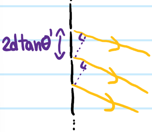
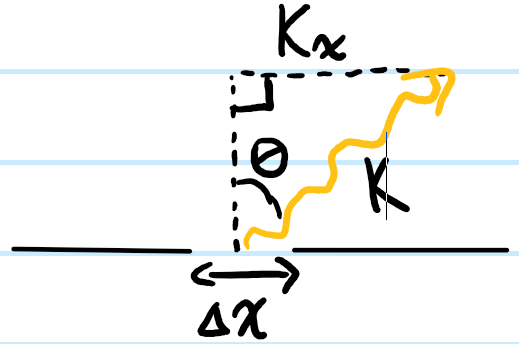
Problem: Show geometrically that the same result applies in a Fabry-Perot interferometer, except the only difference now is that the amplitude is split at transmission/reflection from a low-\(Z\) to high-\(Z\) dielectric, contributing an additional \(\pi\) phase shift not present in the thin-film interferometer, so in total it’s \(2\pi\equiv 0\).
Solution:
One can also view the Fabry-Perot interferometer as a black box in which case it just behaves like a diffraction grating with slit spacing \(2\Delta x\tan\theta’\), though one also has to account for the extra optical path length traversed inside the optical cavity which can be modelled by an effective glass wedge that phase shifts each beam by a constant \(2k’\Delta x/\cos\theta’\) with respect to its nearest neighbours):
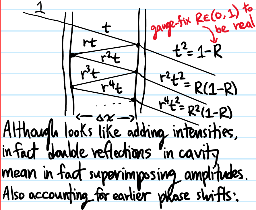
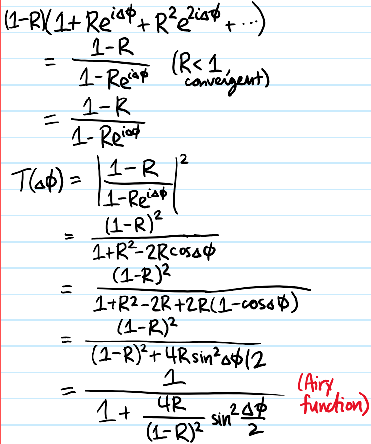
Problem: Now one would like to do better, improving on the previous result. Specifically, one would not only like to know when maxima occur, but also the shape of the FPI’s transmission function \(T(\Delta\phi)\) (i.e. the fraction of the incident power transmitted as a function of the phase shift \(\Delta\phi\) between nearest neighbour reflections). To this end, show that such a transmission function is given by the Airy formula:
where \(R\) is the reflectivity of either mirror (assumed to be identical), and \(\Delta\phi=2k_x’\Delta x\).
Solution:
Problem: Verify using the Airy transmission function the earlier claim in Problem … that maximum constructive interference occurs when \(\Delta\phi=2\pi m\).
Solution: The Airy transmission function \(T(\Delta\phi)\) is maximized when its denominator is minimized, which occurs when the positive semi-definite part is \(0\), i.e. \(\sin\Delta\phi/2=0\Rightarrow\Delta\phi/2=m\pi\Rightarrow\Delta\phi= 2\pi m\).
Problem: From the plot, it is clear that as one polishes the mirrors more, increasing their reflectivity \(R\), the transmission resonances of the Fabry-Perot occurring (as verified in the previous part) at \(\Delta\phi=2\pi m\) are getting sharper and sharper. Quantify this phenomenon by writing down a formula for the width of the peak.
Solution: The peak clearly has a Lorentzian feel to it, and indeed this can be made explicit by Taylor expanding the \(\sin\) function, choosing the \(m=0\) resonance for simplicity (periodicity ensures they are all identical):
Problem: In analogy to the quality factor \(Q\) of a damped harmonic oscillator, define the finesse \(\mathcal F\) of the Fabry-Perot interferometer (it similarly measures the “quality” of the FPI).
Solution: Just as \(Q=\omega_0/\Delta\omega\), one can analogously define:
where the \(2\pi\) can be interpreted in analogy to \(\omega_0\) as being where the first transmission resonance lies (apart from the one at \(\Delta\phi=0\)), though of course this is actually the separation between any pair of nearest neighbour transmission resonances (which one can loosely refer to as the free spectral range \(\Delta\phi_{\text{FSR}}=2\pi\)).
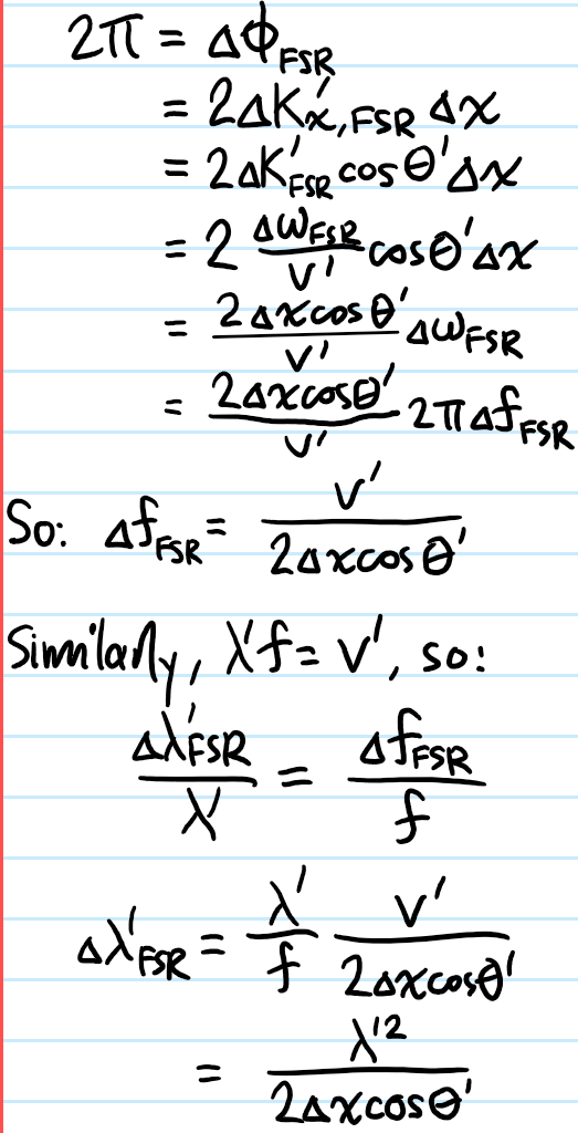
Problem: It is customary to speak of the free spectral range not in \(\Delta\phi\)-space, but when the FPI’s transmission comb is plotted in \(f\)-space or \(\lambda’\)-space. Using \(\Delta\phi_{\text{FSR}}=2\pi\) as the starting point, find expressions for \(\Delta f_{\text{FSR}}\) and \(\Delta\lambda_{\text{FSR}}\) (strictly speaking, a bunch of places where \(\Delta\phi\) is written should really be written as \(\Delta\Delta\phi\) and read as “the difference in delta-phis”)
Solution:
Problem: Although the finesse \(\mathcal F\) was defined in analogy to a \(Q\)-factor in \(\Delta\phi\)-space, show that it also behaves more intimately like a genuine \(Q\)-factor in \(\omega\)-space (and hence also \(f\)-space)!
Problem: The line width \(\Delta\lambda’_{\text{FWHM}}\) is often taken to define a “resolution element” of the FPI in \(\lambda’\)-space. This is because, if the incident light is not monochromatic, but say contains \(2\) closely spaced wavelengths \(\lambda’_1,\lambda’_2\), then the FPI will be able to resolve them at the \(m^{\text{th}}\) order iff:
Now write \(f=f_m\) for the frequency of the \(m^{\text{th}}\) order of the FPI in \(f\)-space. Clearly this is just \(f_m=m\Delta f_{\text{FSR}}\) a sequence of \(m\) hops of the free spectral range \(\Delta f_{\text{FSR}}\). This yields the desired result.
Problem: What does the phrase “spectral line shape” mean?
Solution: A spectrum is typically a plot of the intensity \(I(\omega)\sim|E(\omega)|^2\) of some underlying time domain signal \(E(t)\).
Problem: What are the \(2\) most prominent kinds of spectra one encounters?
Solution: There are both emission spectra and absorption spectra (and also, it seems there are only broadening mechanisms, no such thing as narrowing mechanisms).
Problem: Distinguish between homogeneousbroadening mechanisms and inhomogeneous broadening mechanisms.
Solution: Homogeneous broadening mechanisms affect all atoms indistinguishably, giving rise to a Lorentzian spectral line shape. By contrast, inhomogeneous broadening mechanisms affect atoms distinguishably; this leads to non-Lorentzian spectral broadening.
Problem: In the presence of Doppler broadening alone, what is the spectral line shape?
Solution:Along \(1\)-dimension, the Maxwell-Boltzmann distribution of velocities is normally distributed (no factor of \(4\pi v^2\)):
The non-relativistic Doppler shift gives the angular frequency random variable \(\omega\) as an affine transformation of the velocity random variable \(v\):
In particular it is also a Gaussian (hence Doppler broadening is inhomogeneous) but with expectation \(\omega_0\) and standard deviation (aka line width) \(\Delta\omega\):
(slogan: variance proportional to temperature) so the quality factor \(Q:=\omega_0/\Delta\omega_D\) of depends on the ratio of rest mass energy \(mc^2\) of each particle to their thermal energy \(k_BT\).
Problem: In the presence of natural/lifetime/radiative broadening alone, what is the spectral line shape?
Solution: For a \(2\)-level system with ground state \(|0\rangle\) and excited state \(|1\rangle\) associated to a lifetime \(\tau\) of spontaneous emission, then the natural line width is:
\[\Gamma\sim\omega\sim\frac{1}{\tau}\]
and the spectral line shape is a Lorentzian \(\sim\frac{1}{(\omega-\omega_0)^2+\Gamma^2}\) (is there a clear way to understand why? From optical Bloch equations for instance…). So natural broadening is a homogeneous broadening mechanism.
Problem: In the presence of pressure/collisional broadening alone, what is the spectral line shape?
Solution: Also a Lorentzian as with natural broadening (so also homogeneous), but the line width is determined from the relaxation time \(\tau=\ell/\langle v_{\text{rel}}\rangle\) between collisions. Using the fact that the mean free path is \(\ell=1/n\sigma\), this yields the line width due to pressure broadening:
\[\Delta\omega=n\sigma\langle v\rangle\]
Problem: What does the overall spectral line shape look like when multiple broadening mechanisms are at play?
Solution:
sum of independent random variables yields convolution.
Power Broadening
This is also homogeneous.
Doppler Broadening
Need to use that formula for converting a probability distribution of one random variable into another function of it with the derivative…(this is how you can experimentally verify the Maxwell distribution btw).
Problem: Draw a DNA molecule. Annotate the terms nucleotides, phosphate group, deoxyribose, phosphodiester linkage, adenine, thymine, cytosine, guanine, nitrogenous bases.
Problem: Draw an RNA molecule, and make similar annotations as for DNA.
Problem: What is the typical length scale \(x_{\text{cell}}\) of a cell? How does that compare with the typical width \(x_{\text{hair}}\) of a human hair?
Solution: One has \(x_{\text{cell}}\sim 10\space\mu\text m\), whereas \(x_{\text{hair}}\sim 100\space\mu\text m\), so \(x_{\text{hair}}/x_{\text{cell}}\sim 10\) (though exact values vary!).
Problem: Draw a cartoon cross-section of a typical eukaryotic cell. Annotate the terms nucleus, mitochondria, ribosome, rough endoplasmic reticulum, smooth endoplasmic reticulum, golgi bodies, lysosomes, and (for plants) chloroplasts.
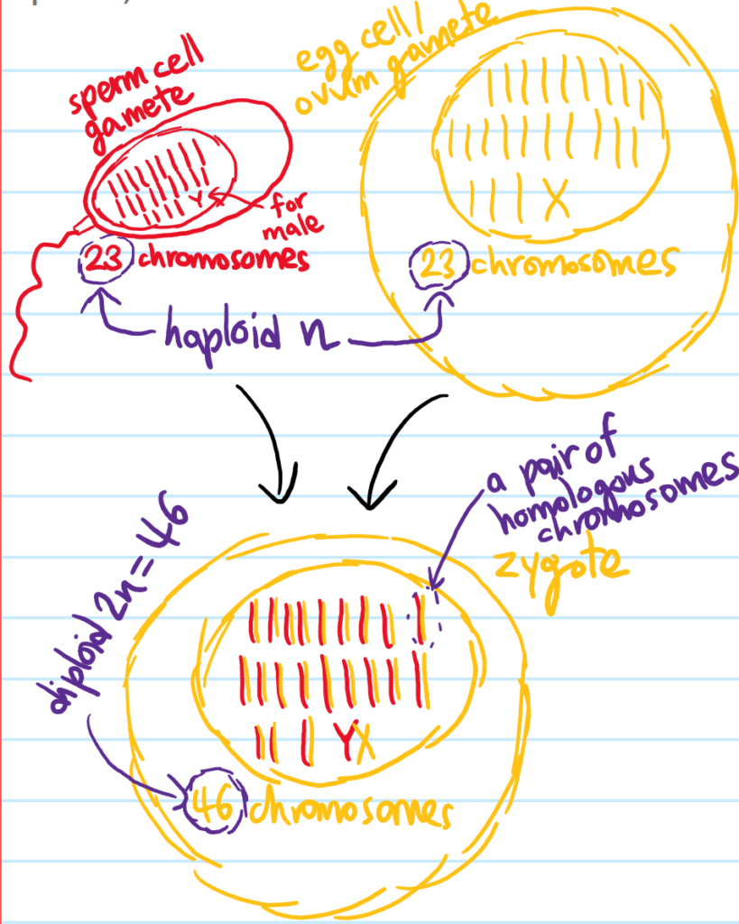
Problem: Draw a diagram depicting the process of fertilization. Annotate the terms gamete, zygote, pair of homologous chromosomes, haploid number, and diploid number on the diagram.
The initial \(t=0\) Bose gas momentum space distribution \(n_{|k\rangle}(t=0)\) is sharply peaked at some \(k=k_0\), with the low-energy bosons of \(k<k_0\) in the so-called IR regime and the high-energy bosons of \(k>k_0\) in the UV regime.
The strongly interacting regime corresponds to bosons with \(k\xi\ll 1\) with \(\xi\propto a^{-1/2}\) the healing length, whereas the weakly interacting regime is \(k\xi\gg 1\).
In the UV regime, if it starts weakly interacting then it will remain like that because \(k\) just grows, pushing further into weakly interacting.
In the IR regime, there is a transition from strongly to weakly interacting, so more interesting to study.
Gevorg’s speed limit paper showed that the coherent coarsening dynamics as quantified by the speed limit \(3\hbar/m\) is, after an initial transient, independent of the (dimensionless) interaction strength \(1/(k\xi)\).
WWT applies to the weakly interacting \(k\xi\gg 1\) regime.
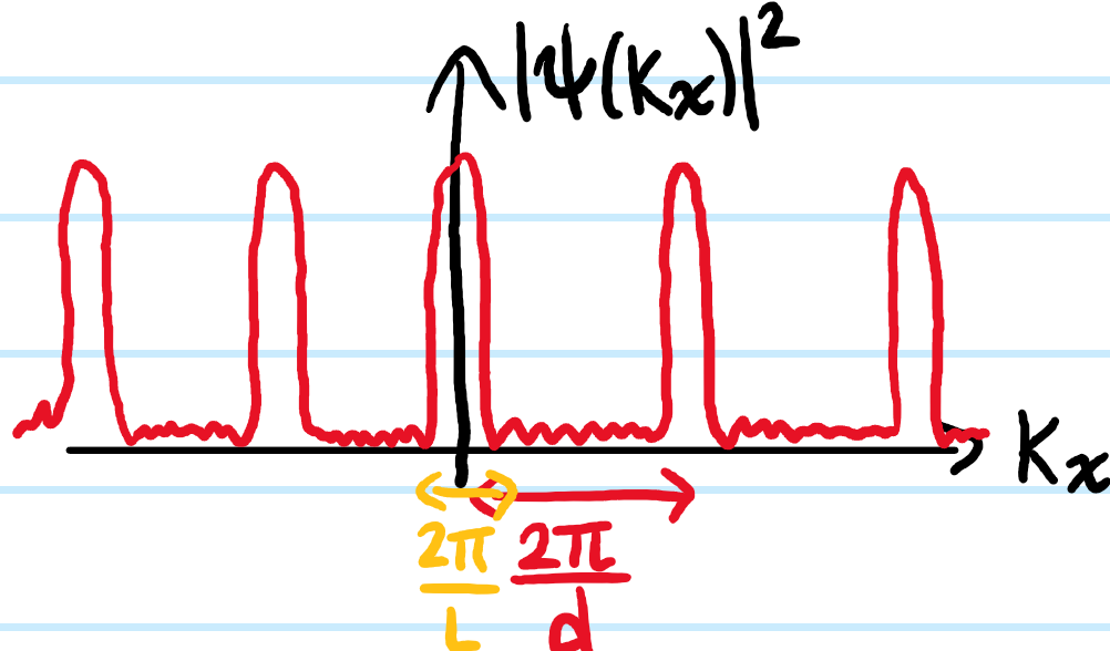
# the wiggles at the end are due to diffraction off the BEC, not the sinc momentum space contribution from the BEC which is approximately(need to crop them from the data)
# a homogeneous top hat in real space.
# Each experimental cycle lasts about 30 seconds, the first 25 seconds is just the standard steps (MOT, evaporation, Sisyphus cooling, molasses, etc.), the last 5 seconds
# only like a few seconds is actually the physics.
# Right now, Gevorg & Simon decided to have 15 increasing TOFs, in order to probe the momentum space distribution n_k of the BEC.
# The idea is that you measure a 2D momentum space distribution of the BEC along your line of sight, then inverse Abel transform (involves a derivative)
# it to get the 3D momentum space distribution. But also, the only part you can reliably inverse Abel transform is the part that is not diffracted
# off the BEC and doesn’t saturate the optical density OD at 3, so can only reliably measure in sort of the “outskirt” regions of the cylinder so to speak
# where the BEC is not too dense (i.e. OD < 3). Also this is why it’s hard to measure the low-k part of the momentum space distribution, b/c the BEC is so dense
# there (OD > 3) that it saturates the imaging system.
# Numerical differentiation is much less robust than numerical integration (Gevorg gave example of a monotonic function like exp(x)),
# so it’s much harder to get the 3D momentum space distribution. In the case of the inverse Abel transform, you have to differentiate by subtracting the
# of neighbouring pixels.
# Need to be on the Cambridge VPN to “SSH” into the VNC viewer to see Analysis GpUI (imaging computer), Cicero, Origin, or any of the office computers
# each of the lab computers has a IP address, and you can only access them from the Cambridge network. Also a remote Toptica software for
# relocking the laser if it drifts/unlocks overnight (somehow not so easy to just automate this b/c need to manually play with the current and piezo voltage in the AOMs).
# Ground state wavefunction of BEC in k-space is not exactly a sinc, rather a Bessel b/c it’s a cylinder.
# one-body loss, evaporative loss, usually temperatures too high cf. box trap depth, in that case lose a lot of energy but not many particles
# b/c only particels you lose are the high-energy ones, so you lose a lot of energy but not many particles
# another worry is counting worry, the n_rad_k distributions might overestimate or underestimate the number of particles
# e.g. the 350000 atoms seems too high…truncate integrals as well to avoid the noisy region at high-k.
# for n_k use log-log, for k**2*n_k or k**4*n_k use lin-lin maybe? or log-lin… advantage of lin-lin is that area you visually see is proportional to the
# integral of the function and for k**2 and k**4 this is nice to see.
#try playing around with some different definition of “speed of thermalization”, see if they give a monotonic thing or not
# also compare with the GPE & WWT theory of the paper (which plots k**2*n_k) see if it matches…
# change energy to temperature scale (nK), also get E/N for each set
Problem: Explain what is meant by a classical field.
Solution: A classical field is any function \(\phi(x)\) (denoted as \(\phi\) because “phi” sounds like “field”) on spacetime \(x:=(ct,\mathbf x)\in\mathbf R^{1,3}\) which is a \(c\)-number, that is to say \(\phi(x)\in\mathbf R\) or \(\phi(x)\in\mathbf C\) or \(\phi(x)\in\mathbf R^4\) or \(\mathbf C^4\) or something like that. Classical fields stand in sharp contrast to quantum fields which are no longer (necessarily) \(c\)-numbers but in general \(q\)-numbers (operator-valued).
Problem: Explain why the words “theory” and “action” are interchangeable, so e.g. if someone says “Klein-Gordan field theory is Lorentz invariant” or “Maxwell’s field theory of classical electromagnetism is both Lorentz invariant and gauge invariant”, it is respectively synonymous with “the Klein-Gordan action is Lorentz invariant” or “the Maxwell action is both Lorentz invariant and gauge invariant”.
Solution: Because once an action \(S\) is written down for a classical field theory, it defines what classical fields are involved in the theory, their dynamics, etc. in other words, a complete specification of all the relevant information.
Problem: Write down the action \(S\) of a classical field theory in terms of its Lagrangian density \(\mathcal L\). State the Lagrangian density \(\mathcal L_{\text{KG}}\) of Klein-Gordan field theory and the Lagrangian density \(\mathcal L_{\text{EM}}\) of Maxwell field theory.
Solution: From classical particle mechanics, \(S=\int dt L\) where \(L=\int d^3\mathbf x\mathcal L\) is the classical Lagrangian. Thus, overall \(S=c^{-1}\int d^{1+3}x\mathcal L\) where the extra factor of \(c\) is to remove the factor of \(c\) in the spacetime measure \(d^{1+3}x=cdtd^3\mathbf x\). Klein-Gordon field theory governs the dynamics of a single real scalar field \(\phi(x)\):
where \(k_c=2\pi/\lambda_c\) is the Compton wavenumber associated to the Compton wavelength \(\lambda_c=h/mc\). The important point is that \(k_c\propto m\). By contrast, Maxwell field theory governs the dynamics of a \(4\)-vector field \(A^{\mu}(x)\):
where the electromagnetic field tensor \(F_{\mu\nu}=\partial_{\mu}A_{\nu}-\partial_{\nu}A_{\mu}\).
Problem: What does it mean for a classical field theory to be Lorentz invariant (aka relativistic)? How can one often instantly tell if a classical field theory is compatible with special relativity or not?
Solution: Loosely speaking, a classical field theory is Lorentz invariant iff its action \(S\) is a Lorentz scalar:
\[\frac{\delta S}{\delta SO^+(1,3)}=0\]
Both Klein-Gordan and Maxwell are relativistic field theories. The giveaway is the presence of Greek spacetime indices like \(\mu,\nu=0,1,2,3\), etc. in their Lagrangian densities \(\mathcal L_{\text{KG}},\mathcal L_{\text{EM}}\) (one calls this phenomenon manifest Lorentz invariance). More precisely, such spacetime indices must be contracted appropriately, thus putting space and time on equal footing.
Problem: More generally, any transformation \((x,\phi_i)\mapsto (x’,\phi’_i)=(x+\delta x,\phi_i+\delta\phi_i)\) of the spacetime coordinates and fields that leaves the action \(S\) invariant is called a symmetry of the classical field theory (perhaps that’s why the action is denoted by the letter \(S\) because it’s screaming “\(S\)ymmetry!”). Explain why finding symmetries is useful.
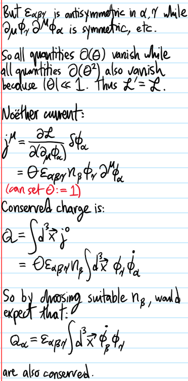
Solution: If the symmetry is continuous, then Noether’s theorem asserts existence of a conserved \(4\)-current. Moreover, the proof is constructive:
where the Jacobian determinant is \(\det\left(\frac{\partial x’}{\partial x}\right)\approx 1+\partial_{\mu}\delta x^{\mu}\) and \(\delta\mathcal L=\frac{\partial\mathcal L}{\partial\phi_i}\delta\phi_i+\frac{\partial\mathcal L}{\partial(\partial_{\mu}\phi_i)}\partial_{\mu}\phi_i+\frac{\partial \mathcal L}{\partial x^{\mu}}\delta x^{\mu}=\partial_{\mu}(\pi^{\mu}_i\delta\phi_i)+(\partial_{\mu}\mathcal L)\delta x^{\mu}\) (where \(\pi^{\mu}_i:=\frac{\partial\mathcal L}{\partial (\partial_{\mu}\phi_i)}\)). Hence, the action variation is the spacetime integral of a spacetime divergence:
Here, \(\delta\phi_i:=\phi’_i(x)-\phi_i(x)\) is the local variation of \(\phi_i\) at a fixed event \(x\in\mathbf R^{1,3}\). It can be related to the net variation \(\Delta\phi_i:=\phi’_i(x’)-\phi_i(x)\) due to both internal transformations and induced variation arising from the coordinate transformation \(\delta x\) using \(\delta\phi_i=\Delta\phi_i-\delta x^{\mu}\partial_{\mu}\phi_i\). This allows the Noether current to be rewritten:
with canonical stress-energy tensor field \(T^{\mu}_{\nu}=\pi^{\mu}_i\partial_{\nu}\phi_i-\delta^{\mu}_{\nu}\mathcal L\) or equivalently \(T^{\mu\nu}=\pi^{\mu}_i\partial^{\nu}\phi_i-g^{\mu}_{\nu}\mathcal L\)
(in particular, notice that \(\delta\mapsto g\)).
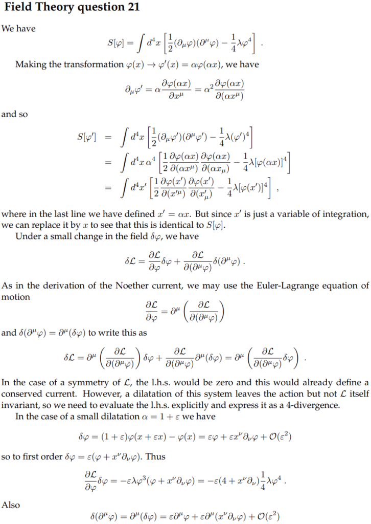
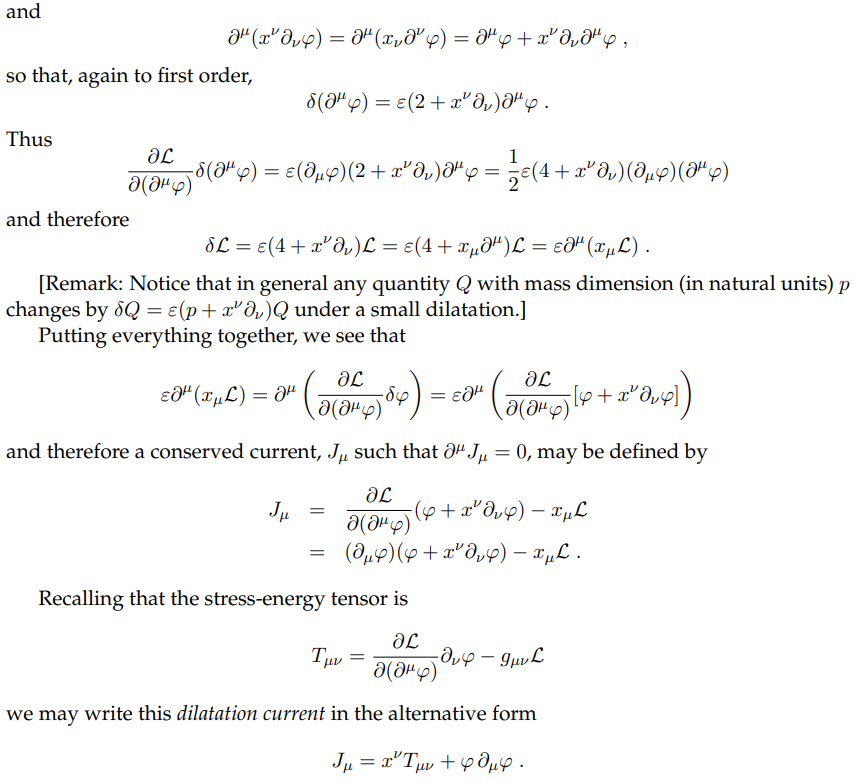
Problem: Consider a classical field theory (massless \(\phi^4\)) involving a single real scalar field \(\phi(x)\) with action:
Show that the conformal dilatation transformation \(\phi(x)\mapsto\alpha\phi(\alpha x)\) for \(\alpha\in\mathbf R\) is a continuous symmetry of this classical field theory, and hence compute the associated Noether current.
Solution: The hardest part of this problem is to understand precisely what the notation \(\phi(x)\mapsto\alpha\phi(\alpha x)\) means. The answer is that it simultaneously defines a spacetime transformation \(x\mapsto x’=x/\alpha\) and a corresponding active field transformation \(\phi(x)\mapsto \phi'(x)=\alpha\phi(\alpha x)\), so in particular \(\phi'(x’)=\alpha\phi(x)\). To check invariance of the action \(S\):
which is consistent with \(\Delta\phi=\delta\phi+\delta x^{\nu}\partial_{\nu}\phi\). The conserved Noether current is thus (using the form with the stress-energy tensor):
(aside: it is instructive to explicitly check \(\partial_{\mu}j^{\mu}=0\) by working on-shell \(\partial^{\mu}\partial_{\mu}\phi=-\lambda\phi^3\) and also invoking spacetime translational symmetry \(\partial_{\mu}T^{\mu}_{\nu}=0\)).
Problem: Continuing with the classical massless \(\phi^4\) field theory:
also preserve the action \(S\), hence are symmetries of the theory. Compute their associated Noether currents.
Solution:
This perspective is implicitly adopted in the Cambridge Theoretical Physics course official solution for this problem:
However, since \(\delta x=0\), this approach suggests an incorrect Noether current \(j^{\mu}=\pi^{\mu}\delta\phi=\phi\partial^{\mu}\phi+x^{\nu}\partial_{\nu}\phi\partial^{\mu}\phi\). Rather, as the solution above suggests, one has to compute the corresponding change in the infinitesimal action \(d^{1+3}x’\mathcal L’-d^{1+3}x\mathcal L=d^{1+3}x(\alpha-1)\partial_{\mu}(x^{\mu}\mathcal L)\), hence giving the required subtractive correction.
2. This transformation is just a trivial renaming of the integration dummy variable from \(x\) to \(x’=\alpha x\) (indeed, it could be renamed to any reasonable \(x’=f_{\alpha}(x)\) with corresponding \(\phi'(x’)=\phi(f_{\alpha}(x))\)):
In particular, \(\phi'(x)=\phi(x)\) and thus \(\delta\phi=0\). The transformation of course has nothing to do with the conformal dilatation of the massless \(\phi^4\) field. Contrary to the previous situation, the formula now predicts an incorrect Noether current \(j^{\mu}=x^{\mu}\mathcal L\). Applying the same correction as above yields the trivial Noether current \(0\).
The lesson here is that one should always write the transformed field \(\phi'(x’)\) in terms of \(\phi(x)\), and in particular not \(\phi(\alpha x)\) or any other \(\phi(f(x))\). Then the earlier Noether current result applies.
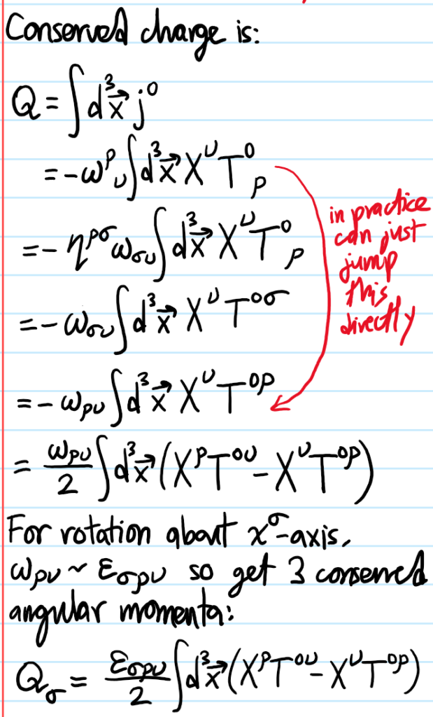
Problem: Explain how to calculate the orbital angular momentum pseudovector \(\mathbf L\) of a classical field.
Solution: Recall that spatial rotations \(SO(3)\) form a subgroup of the Lorentz group \(SO^+(1,3)\). Thus, when traditionally working with an infinitesimal Lorentz transformation \(\Lambda^{\mu}_{\nu}=\delta^{\mu}_{\nu}+\omega^{\mu}_{\nu}\), this procedure simultaneously yields conservation laws for both spatial rotations and Lorentz boosts. One has \(\Lambda\in SO^+(1,3)\) iff the generator \(\omega_{\mu\nu}=-\omega_{\nu\mu}\) is antisymmetric (hence denoted by the symbol “\(\omega\)”). Thus, \(x’^{\mu}=\Lambda^{\mu}_{\nu}x^{\nu}\approx x^{\mu}+\omega^{\mu}_{\nu}x^{\nu}\) and \(\Delta\phi=0\) because \(\phi'(x’)=\phi(x)\) is a scalar field. One has:
where the orbital angular momentum density tensor field is \(L^{\mu\nu\rho}:=c^{-1}(x^{\nu}T^{\mu\rho}-x^{\rho}T^{\mu\nu})\). There are \(6\) combinations of \(\nu,\rho\in\{0,1,2,3\}\) for which \(\omega_{\nu\rho}\neq 0\), giving \(6\) conserved currents \(\partial_{\mu}L^{\mu\nu\rho}=0\), with the conserved charge \(L^{\mu\nu}=\int d^3\mathbf x L^{0\mu\nu}(x)\). By antisymmetry \(L^{\nu\mu}=-L^{\mu\nu}\), the spatial parts can be identified with a \(3\)-vector in the usual way \(L^i:=\frac{\varepsilon_{ijk}}{2}L^{jk}\); this is the orbital angular momentum pseudovector \(\mathbf L\) of the field.
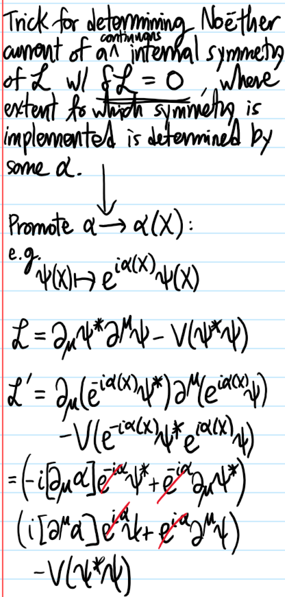
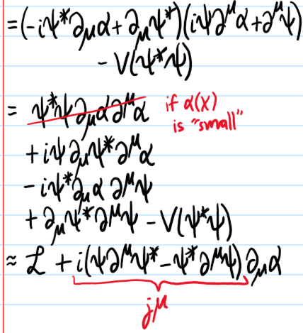
Problem: Consider a classical field theory involving a complex scalar field \(\psi(x)\). Write down the Lagrangian density \(\mathcal L(\psi)\) for \(\psi\) such that:
where the Klein-Gordon Lagrangian density for a real scalar field \(\phi(x)\) is \(\mathcal L_{\text{KG}}(\phi):=\frac{1}{2}\partial^{\mu}\phi\partial_{\mu}\phi-\frac{1}{2}k_c^2\phi^2\). Suppose \(\psi\) is coupled to an electromagnetic field \(A^{\mu}\); describe how \(\mathcal L(\psi)\) needs to be modified to account for this.
Solution: It’s just a “Hermitian” version of Klein-Gordon, without the factors of \(1/2\):
Typically one just writes \((\partial^{\mu}\psi)^{\dagger}=\partial^{\mu}\psi^{\dagger}\) because \((\partial^{\mu})^{\dagger}=\) is Hermitian, but it will soon be important to remember that the dagger \(\dagger\) is meant to act on the entire object.
When \(\psi\) is coupled to an electromagnetic \(4\)-potential \(A^{\mu}\), there are \(2\) changes one must make to \(\mathcal L(\psi)\); the obvious one is to also tack on \(\mathcal L_{\text{EM}}=-F^{\mu\nu}F_{\mu\nu}/4\mu_0\). The more subtle one is the minimal coupling substitution in the kinetic term \(\partial\mapsto\mathcal D:=\partial-iqA/\hbar\) with \(\mathcal D\) the gauge covariant derivative.
Although inspired by the classical minimal coupling \(\mathbf p\mapsto\mathbf p-q\mathbf A\), the reason for this has to do with desiring \(\mathcal L\) to be invariant under a simultaneous local \(U(1)\) phase transformation of the complex scalar field \(\psi(x)\mapsto\psi'(x’)=e^{i\theta(x)}\psi(x)\) in conjunction with a gauge transformation of \(A(x)\mapsto A'(x’)=A(x)+\frac{\hbar}{q}\partial\theta(x)\) (in both cases, \(x’=x\)), then:
\[\mathcal D’\psi’=e^{i\theta}\mathcal D\psi\]
Thus, the kinetic term is invariant \((\mathcal D’\psi’)^{\dagger}\mathcal D’\psi’=e^{-i\theta}e^{i\theta}(\mathcal D\psi)^{\dagger}\mathcal D\psi=(\mathcal D\psi)^{\dagger}\mathcal D\psi\). Equivalently, one can say that if the gauge field is transformed as \(A\mapsto A+\partial\Gamma\), then the scalar field must transform with a local phase \(\psi\mapsto e^{iq\Gamma/\hbar}\psi\).
Problem: Consider the ungauged Lagrangian density:
Consider using the Mexican hat potential \(V(\psi)=-k_c^2|\psi|^2+\frac{\lambda}{2}|\psi|^4\) with \(k_c^2,\lambda>0\). Explain both of these inequalities.
Write down the general ground state \(\psi_0\), and “quadraticize” (cf. “linearize”) \(\mathcal L\) about \(\psi_0\). Identify the massless Goldstone field. By promoting global to local \(U(1)\) phase symmetry to hold for the theory, the idea of coupling to a gauge field \(A(x)\) emerges naturally (scalar electrodynamics):
Show that the gauge field \(A(x)\) acquires a mass by eating the Goldstone field via the abelian Higgs mechanism.
Solution: The need to make \(\lambda>0\) arises from insisting that \(V(\psi)\in\mathbf R\) is bounded from below (otherwise \(|\psi|\to\infty\) would be unphysical), so in particular at least \(1\) global minimum exists (called a ground field/”state”). In addition, the negative coefficient \(-k_c^2\) on the quadratic term is the opposite of the positive coefficient \(k_c^2\) that normally appears in Klein-Gordan type Lagrangian densities; this is to mimic ordering behavior in contexts like continuous phase transitions where \(T<T_c\)).
By insisting \(\partial V/\partial |\psi|^2=0\), one obtains \(\psi_0=\frac{k_c}{\sqrt{\lambda}}e^{i\phi}\) for arbitrary phase \(\phi\in\mathbf R\). By settling into a specific angle \(\phi\), the system spontaneously breaks the continuous rotational symmetry of \(V(\psi)\). Due to the global \(U(1)\) phase symmetry of the theory, one can simply rotate away the phase \(\phi\) and henceforth w.l.o.g. work with a real vacuum expectation value \(\psi_0=\frac{k_c}{\sqrt{\lambda}}\in\mathbf R\). However, this is just an expectation value; there will be fluctuations about it. One can consider both radial fluctuations \(h(x)\) and azimuthal fluctuations \(g(x)\), leading to the ansatz \(\psi(x)=\psi_0+h(x)+ig(x)\). Plugging into \(\mathcal L\) and discarding cubic or higher-order terms:
So the radial fluctuation field \(h(x)\) (called the Higgs field) is massive in the sense that after quantization, its particles will have mass \(m_h=\sqrt{2}m\) (where \(m=\hbar k_c/c\)) and dispersion relation \(\omega_k=c\sqrt{k^2+2k_c^2}\). By contrast, the azimuthal fluctuation field \(g(x)\) (called the Goldstone field) is massless \(m_g=0\) because of the absence of an associated \(g^2\) term in \(\mathcal L\). It is therefore like a photon \(\omega_k=ck\) (except it is spin-\(0\) whereas photons are spin-\(1\)). These notions are all pretty intuitive if one conceptualizes mass as a kind of “stiffness” of moving in certain directions in the potential energy landscape \(V(\psi)\); clearly it requires more energy to move radially rather than azimuthally in a Mexican hat \(V(\psi)\) when sitting at the trough \(\psi_0\).
The Higgs mechanism essentially amounts to FOILing the gauge-invariant kinetic term:
and noticing that it gives an \(\sim A^2\) mass-like term.
Problem: Outline the isomorphism between classical particle mechanics and classical field theory (indeed, leveraging one’s prior experience with classical particle mechanics is the best way to bridge towards an understanding of classical field theory).
Solution: In classical particle mechanics, the dynamical degrees of freedom are the particle trajectories \(\mathbf x_1(t),…,\mathbf x_N(t)\). By contrast, in classical field theory, the dynamical degrees of freedom are the classical fields \(\phi_1(x),…,\phi_N(x)\). The analogy is thus:
\[t\Leftrightarrow x=(ct,\mathbf x)\]
\[\mathbf x\Leftrightarrow\phi\]
In particular, whereas \(\mathbf x\) is the dynamical degree of freedom in particle mechanics, it is demoted to a mere label in classical field theory for the fields \(\phi_i=\phi_i(\mathbf x,t)\).
Problem: The \(i=1,…,N\) Euler-Lagrange equations of motion for a classical field theory governed by a \(1^{\text{st}}\)-order Lagrangian density \(\mathcal L\) are typically written:
Does the presence of the Greek spacetime index \(\mu=0,1,2,3\) imply that this field theory is relativistic?
Defining the Lagrangian \(L:=\int d^3\mathbf x\mathcal L\), write down the analog of the Euler-Lagrange equations for \(L\) rather than \(\mathcal L\). Similarly, given the Hamiltonian density \(\mathcal H:=\pi^0_i\dot{\phi}_i-\mathcal L\) and the Hamiltonian \(H:=\int d^3\mathbf x\mathcal H\), write down Hamilton’s equations at the level of both \(\mathcal H\) and \(H\); is there an analog of the Legendre transform that relates \(L\) and \(H\)?
Solution: The presence of the Greek spacetime index \(\mu=0,1,2,3\) does not imply anything relativistic about the corresponding field theory, it’s merely a convenient way to write the spacetime divergence that emerges naturally from the chain rule. Thus, it’s unfortunately very misleading.
The Euler-Lagrange equations for \(L\) look very similar to their classical counterpart:
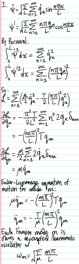
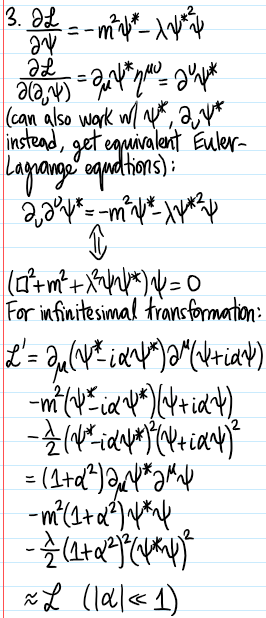
Problem: A string of length \(L\), mass per unit length \(\mu\), under uniform tension \(T\) is fixed at each end. The Lagrangian \(\mathcal L\) governing the time evolution of the transverse displacement \(\psi(x,t)\) is:
Write down the Euler-Lagrange field equations for this system. Verify that the Lagrangian density \(\mathcal L\) is invariant under the infinitesimal transformation:
\[\delta\psi=i\alpha\psi\]
\[\delta\psi^*=-i\alpha\psi^*\]
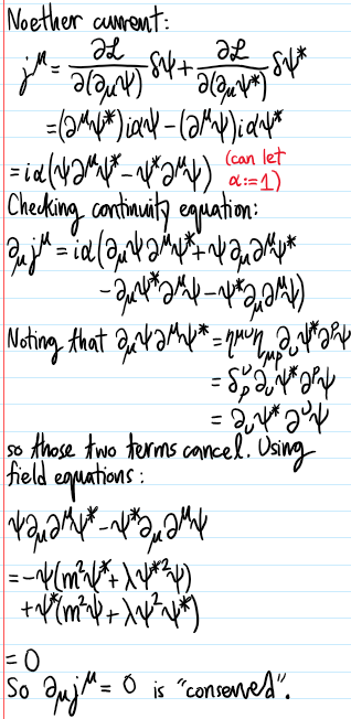
Derive the Noether current \(j^{\mu}\) associated with this transformation and verify explicitly that it is conserved using the field equations satisfied by \(\psi\).
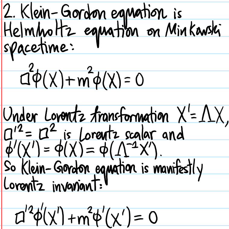
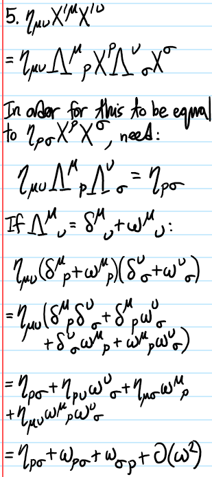
Problem: By requiring that Lorentz transformations \(\Lambda^{\mu}_{\space\space\nu}\) should preserve the Minkowski norm of \(4\)-vectors \(\eta_{\mu\nu}X’^{\mu}X’^{\nu}=\eta_{\mu\nu}X^{\mu}X^{\nu}\), show that this implies:
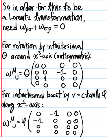
Show that an infinitesimal transformation of the form \(\Lambda^{\mu}_{\space\space\nu}=\delta^{\mu}_{\space\space\nu}+\omega^{\mu}_{\space\space\nu}\) is specifically a Lorentz transformation iff \(\omega_{\mu\nu}=-\omega_{\nu\mu}\) is antisymmetric.
Write down the matrix for \(\omega^{\mu}_{\space\space\nu}\) corresponding to an infinitesimal rotation by angle \(\theta\) around the \(x^3\)-axis. Do the same for an infinitesimal Lorentz boost along the \(x^1\)-axis by velocity \(v\).
Solution:
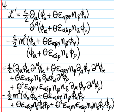
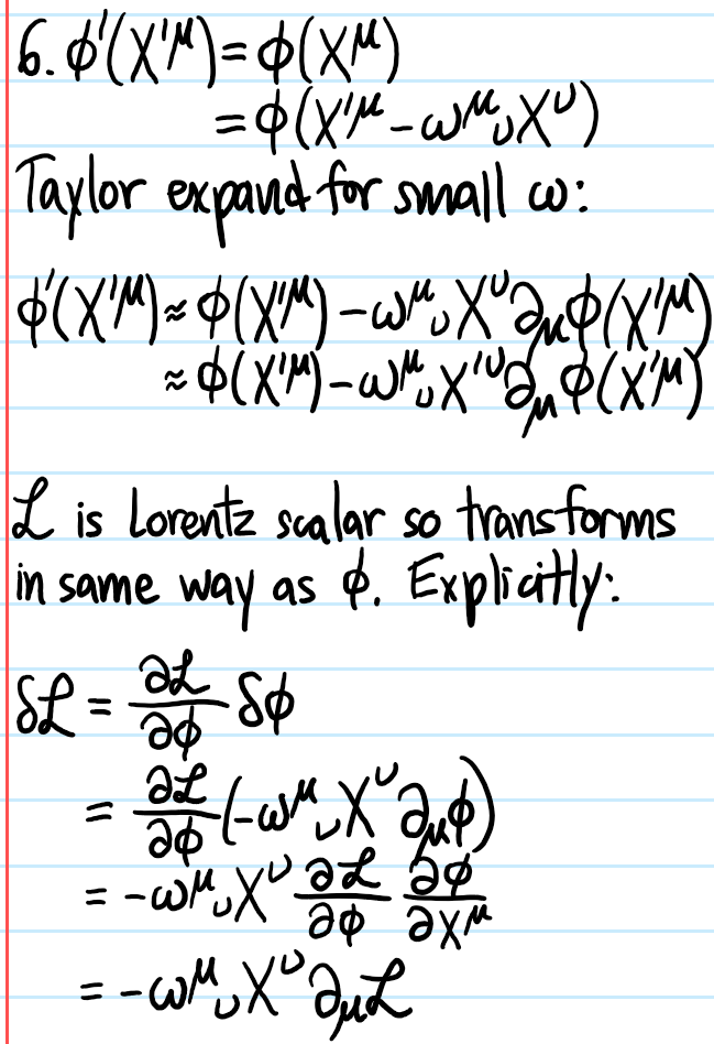
Problem: Consider a general infinitesimal Lorentz transformation \(X^{\mu}\mapsto X’^{\mu}=X^{\mu}+\omega^{\mu}_{\space\space\nu}X^{\nu}\) acting at the level of the \(4\)-vector \(X\). How does this perturbation manifest at the level of a scalar field \(\phi=\phi(X)\)? What about at the level of the Lagrangian density \(\mathcal L=\mathcal L(\phi)\)? What about at the level of the action \(S=S(\mathcal L)\)? In particular, show that the perturbation \(\delta\mathcal L\) at the level of \(\mathcal L\) is a total spacetime derivative, and hence describe the Noetherian implication of this.
Solution:
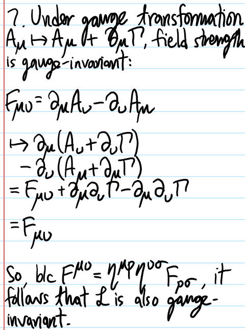
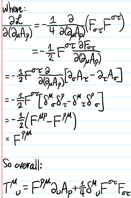
Problem: Maxwell’s Lagrangian for the electromagnetic field is:
\[\mathcal L=-\frac{1}{4}F_{\mu\nu}F^{\mu\nu}\]
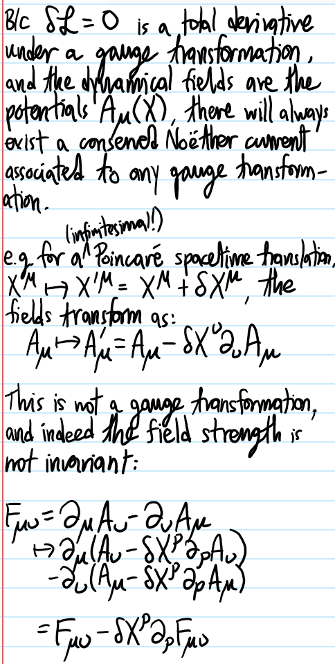
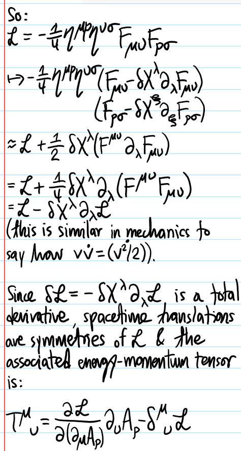
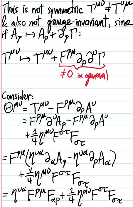
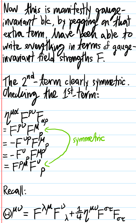
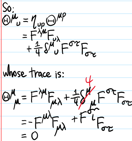
where \(F_{\mu\nu}=\partial_{\mu}A_{\nu}-\partial_{\nu}A_{\mu}\) and \(A_{\mu}\) is the \(4\)-vector potential. Show that \(\mathcal L\) is invariant under gauge transformations \(A_{\mu}\mapsto A_{\mu}+\partial_{\mu}\Gamma\) where \(\Gamma=\Gamma(X)\) is a scalar field with arbitrary (differentiable) dependence on \(X\). Use Noether’s theorem, and the spacetime translational invariance of the action \(S\) to construct the energy-momentum tensor \(T^{\mu\nu}\) for the electromagnetic field. Show that the resulting object is neither symmetric nor gauge invariant. Consider a new tensor given by:
was analyzed (there the potential \(V\) was taken to be analytic in \(\psi^*\psi\) and so Taylor expanded to quadratic order). In particular, the Noether current \(j^{\mu}\) was obtained explicitly for the continuousglobal, internal \(U(1)\) \(\mathcal L\)-symmetry \(\psi\mapsto e^{i\alpha}\psi\) for a constant \(\alpha\in\textbf R\). By promoting \(\alpha=\alpha(X)\) but still acting infinitesimally across \(X\) in spacetime, recompute the Noether current \(j^{\mu}\), and notice in particular that the Noether current \(j^{\mu}\) doesn’t care about the potential terms \(V(\psi^*\psi)\), only the kinetic terms.
Consider an atomic two-level system with ground state \(|0\rangle\) and excited state \(|1\rangle\). Recall that in the interaction picture, after making the rotating wave approximation and boosting into a steady-state rotating frame, one had the resultant time-independent steady-state Hamiltonian:
Invoking the identity of Pauli matrices \((\tilde{\boldsymbol{\Omega}}\cdot\boldsymbol{\sigma})^2=|\tilde{\boldsymbol{\Omega}}|^21\), it is clear that the eigenvalues of this Hamiltonian are thus \(E_{\pm}=\pm\frac{\hbar|\tilde{\boldsymbol{\Omega}}|}{2}=\frac{\hbar\sqrt{\Omega^2+\delta^2}}{2}\), and this is known as the light shift resulting from the AC Stark effect (also called the Autler-Townes effect). In particular, if \(\Omega=0\) then \(E_{\pm}=\).
It is not a coincidence that this light shift calculated from time-independent perturbation theory, after a first-order binomial expansion, to the result of first-order nondegenerate time-independent perturbation theory applied to … turns out in the framework of QED that these correspond to so-called dressed states of the atom-photon system.
The purpose of this post is to explain the \(2\) key models of classical optics, namely geometrical optics (also known as ray optics) and physical optics (also known as wave optics). Although historically geometrical optics came before physical optics, and indeed this is also usually the order in which they are conventionally taught, this post will take the more unconventional approach of presenting physical optics first, and then showing how it reduces to geometrical optics in the \(\lambda\to 0\) limit.
Physical Optics
Discuss:
Fourier optics in the Fraunhofer regime.
Gaussian (pilot) beams
TE/TM/TEM modes in EM waveguides
How Fresnel diffraction is an exact solution to the paraxial Helmholtz equation and what this has to do with the eikonal approximation/Hamilton-Jacobi equation from classical dynamics.
Maxwell’s equations assert that the electric and magnetic field \(\textbf E,\textbf B\) satisfy vector wave equations in vacuum:
Any of their \(6\) components (denoted \(\psi\)) thus satisfy the scalar wave equation \(|\frac{\partial}{\partial\textbf x}|^2\psi+\frac{1}{c^2}\ddot{\psi}=0\). The spacetime Fourier transform yields the trivial dispersion relation \(\omega=ck\) from which it is evident that performing just a temporal Fourier transform (to avoid the minutiae of \(t\)-dependence) leads to the scalar Helmholtz equation for \(\psi(\textbf x)\):
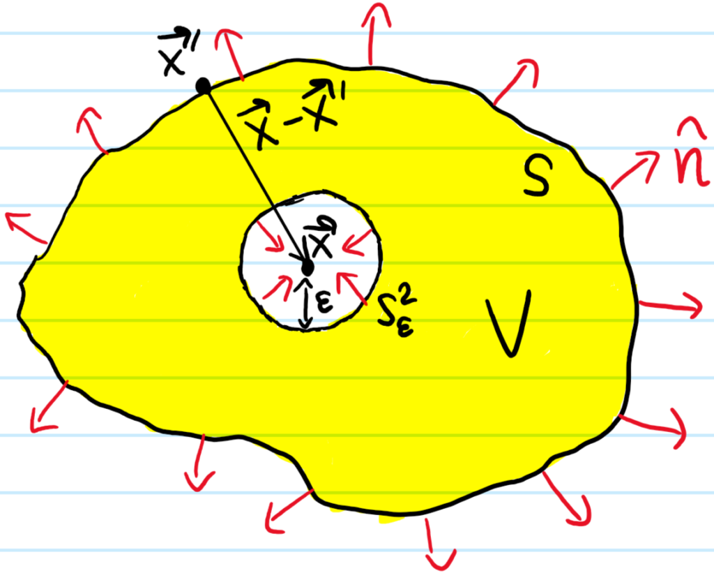
In other words, one is looking for eigenfunctions of the Laplacian \(\biggr|\frac{\partial}{\partial\textbf x}\biggr|^2\) with eigenvalue \(-k^2\). To begin, consider one of Green’s identities, valid for arbitrary scalar fields \(\psi(\textbf x’),\tilde{\psi}(\textbf x’)\) which are \(C^2\) everywhere in the volume \(V\):
(it’s just the divergence theorem applied to the vector field \(\psi\frac{\partial\tilde{\psi}}{\partial\textbf x’}-\tilde{\psi}\frac{\partial\psi}{\partial\textbf x’}\)). It is now obvious that the volume integral will vanish if one then imposes that both \(\psi(\textbf x’)\) and \(\tilde{\psi}(\textbf x’)\) also satisfy the scalar Helmholtz equation. Given any point \(\textbf x\in\textbf R^3\), it is physically clear that the spherical wave Green’s function \(\tilde{\psi}(\textbf x’|\textbf x)=e^{ik|\textbf x-\textbf x’|}/|\textbf x-\textbf x’|\) is one possible (though certainly not a unique) solution to the scalar Helmholtz equation, provided one stays away from thesingularity at \(\textbf x’=\textbf x\). This motivates the choice of volume \(V\) to be some arbitrary region but with an \(\varepsilon\)-ball cut around \(\textbf x\), in which case the volume integral can legitimately be taken to vanish over this choice of \(V\). In that case, the surface \(\partial V=S^2_{\varepsilon}\cup S\) can be partitioned into an inner surface \(S^2_{\varepsilon}\) and an outer surface \(S\):
The flux through these two surfaces \(S^2_{\varepsilon},S\) must thus be equal:
The integral over \(S^2_{\varepsilon}=\{\textbf x’\in\textbf R^3:|\textbf x’-\textbf x|=\varepsilon\}\) is straightforward in the limit \(\varepsilon\to 0\):
As an aside, Kirchoff’s integral formula is very similar in spirit to another more well-known integral formula, namely the Cauchy integral formula \(f(z_0)=\frac{1}{2\pi i}\oint_{z\in\gamma:z_0\in\text{int}(\gamma)}\frac{f(z)}{z-z_0}dz\) from complex analysis; the constraint of complex analyticity is analogous to constraining \(\psi\) to obey the Helmholtz equation; if one specifies both Dirichlet and Neumann boundary conditions for \(\psi(\textbf x’)\) everywhere on \(\textbf x’\in S\), then in principle this is enough to uniquely determine \(\psi(\textbf x)\) everywhere in the interior \(V\) of the enclosing surface \(S\).
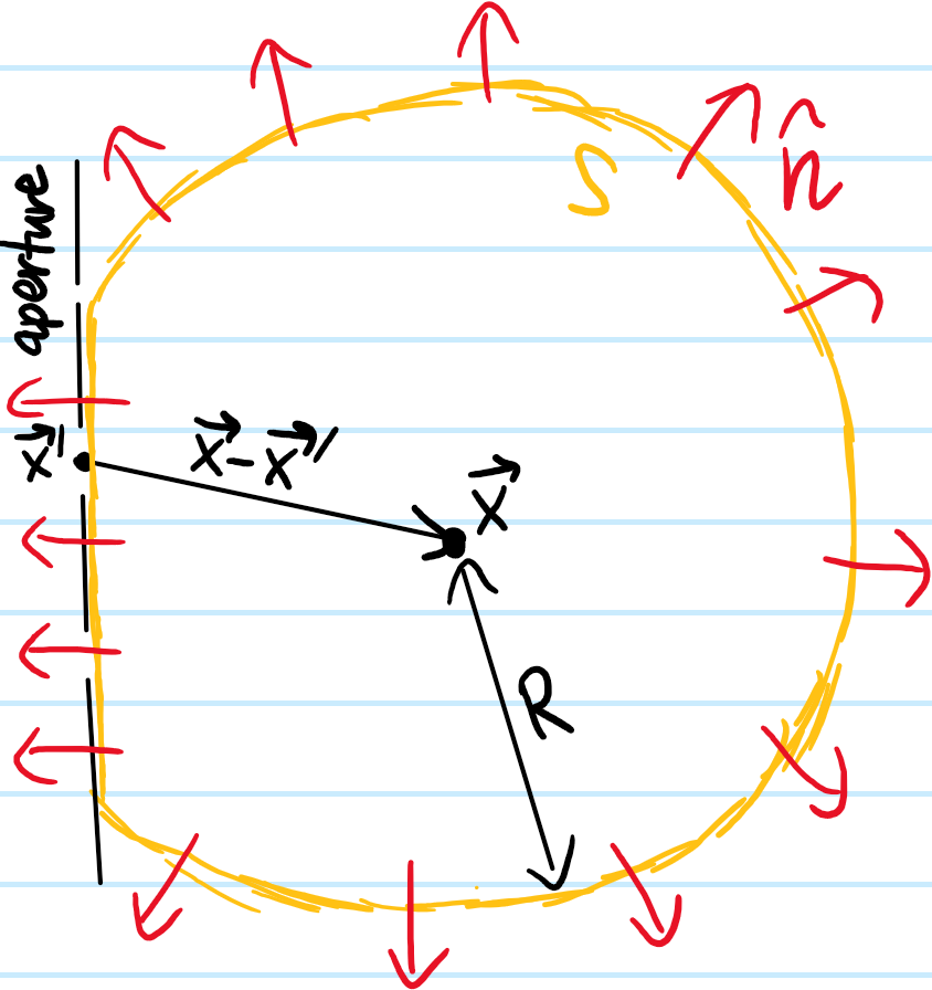
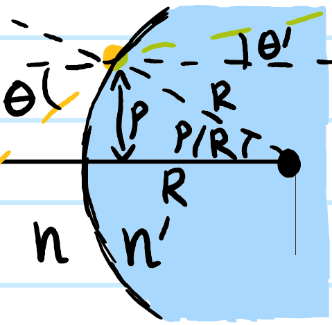
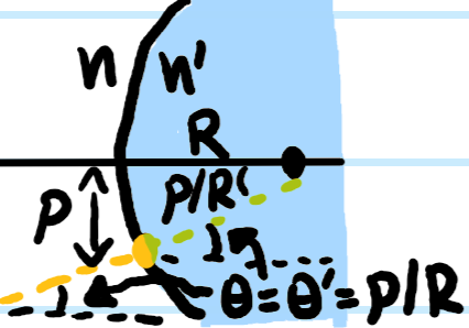
Now consider the following standard diffraction setup:
Here the surface \(S\) is chosen to be a sphere of radius \(R\) centered at \(\textbf x\), except where it flattens along the aperture with some distribution of slits. As one takes \(R\to\infty\), then in analogy to Jordan’s lemma from complex analysis, one can argue that the flux through this spherical cap portion of \(S\) in Kirchoff’s integral formula vanishes like \(\sim 1/R\to 0\) (this is admittedly still a bit handwavy, for a rigorous argument see the Sommerfeld radiation condition). Thus, the behavior of \(\psi\) on the aperture alone is sufficient to determine its value \(\psi(\textbf x)\) at an arbitrary “screen location” \(\textbf x\) beyond the aperture. Supposing a monochromatic plane wave \(\psi(\textbf x’)=\psi(x’,y’,0)e^{ikz’}\) of momentum \(k\) (hence solving the scalar Helmholtz equation) is normally incident on the aperture \(z’=0\) and that \(k|\textbf x-\textbf x’|\gg 1\) (easily true in most cases), this imposes the boundary condition \(-\frac{\partial\psi}{\partial z’}(x’,y’,0)=-ik\psi(x’,y’,0)\) so one can check that Kirchoff’s integral formula simplifies to:
where the obliquity kernel is \(K(\textbf x-\textbf x’):=\frac{1+\cos\angle(\textbf x-\textbf x’,\hat{\textbf k})}{2}=\cos^2\frac{\angle(\textbf x-\textbf x’,\hat{\textbf k})}{2}\). This is nothing more than a mathematical expression of the Huygens-Fresnel principle.
Fresnel vs. Fraunhofer Diffraction
In general the Huygens-Fresnel integral is difficult to evaluate analytically for an arbitrary point \(\textbf x\) on a screen. Thus, one often begins by making the paraxial approximation \(K(\textbf x-\textbf x’)\approx 1\iff |\textbf x-\textbf x’|\approx z\), except in the complex exponential (otherwise all Huygens wavelets would interfere constructively which is silly). Here instead, one implements a less strict version of the paraxial approximation in the form of a \(z^2\gg |\textbf x-\textbf x’|^2-z^2\) binomial expansion:
In practice the quadratic term is negligible in the paraxial limit, so neglecting it and all higher-order terms yields the Fresnel diffraction integral:
where \(\textbf k=k\textbf x/z\). If in addition one also assumes that \(k|\textbf x’|^2/2z\ll 1\), then one obtains the Fourier optics case of far-field/Fraunhofer diffraction:
The reason that Fraunhofer diffraction is only considered to apply in the far-field is that the above condition for its validity can be rewritten as \(z\gg z_R\) where \(z_R:=\rho’^2/\lambda\) is the Rayleigh distance of an aperture of typical length scale \(\rho’\sim\sqrt{x’^2+y’^2}\) when illuminated by monochromatic light of wavelength \(\lambda\). In other words, the precise meaning of “far-field” is “farther than the Rayleigh distance \(z_R\)”. Otherwise, when \(z≲z_R\) then such a term cannot be neglected and one simply refers to it as Fresnel diffraction. Notice that \(z≲z_R\) is not saying the same thing as \(z\ll z_R\); it is often said that Fresnel diffraction is the regime of near-field diffraction but that phrase can be misleading because it suggests that \(z\) can be arbitrarily small, yet clearly at some point if one kept decreasing \(z\) then eventually the higher-order terms in the binomial expansion would also start to matter (moreover, the paraxial approximation would also start to break down). Instead of calling it “near-field diffraction”, a more accurate name for Fresnel diffraction would be “not-far-enough diffraction” \(z≲z_R\). By contrast, Fraunhofer diffraction truly is arbitrarily far-field \(z\gg z_R\). Of course nothing stops one from also considering the case \(z\ll z_R\), there just doesn’t seem to be any special name given to this regime and in practice it’s not as relevant. Finally, sometimes one also encounters the terminology of the Fresnel number \(F(z):=z_R/z\); in this jargon, Fraunhofer diffraction occurs when \(F(z)\ll 1\) whereas Fresnel diffraction occurs when \(F(z)≳1\).
In practice, one typically ignores the pre-factor in front of the aperture integrals since it is the general profile of the irradiance \(|\psi(\textbf x)|^2\) that is mainly of interest. In this case, particular for Fraunhofer diffraction, one can write \(\hat{\psi}(\textbf k)\equiv\psi(\textbf x)\) as just the \(2\)D spatial Fourier transform of the aperture.
Diffraction Through a Single Slit
Consider a single \(y\)-invariant slit of width \(\Delta x\) centered at \(x’=0\). Then the Fraunhofer interference pattern has the form:
Although in general such an integral needs to be evaluated numerically, there is a simple geometric way to gain some intuition for how \(\psi(x)\in\textbf C\) behaves at fixed \(z≲z_R\sim\Delta x^2/\lambda\) via the Cornu spiral (also called the Euler spiral in contexts outside of physical optics). The idea is to shift the \(x\)-dependence from the integrand into the limits via the substitution \(\pi t’^2/2:=k(x-x’)^2/2z\iff t’=\sqrt{\frac{2}{\lambda z}}(x-x’)\). Then, ignoring chain rule factors, one has:
where the limits are \(t’_1(x)=\sqrt{\frac{2}{\lambda z}}(x+\Delta x/2)\) and \(t’_2(x)=\sqrt{\frac{2}{\lambda z}}(x-\Delta x/2)\). Written in terms of the normalized Fresnel integral \(\text{Fr}(t):=\int_0^{t}e^{i\pi t’^2/2}dt’\):
The object \(\text{Fr}(t)\) is a trajectory in \(\textbf C\) which is the aforementioned Cornu spiral:
where one can check the limits \(\lim_{t\to\pm\infty}\text{Fr}(t)=\pm(1+i)/2\). Noting that \(\dot{\text{Fr}}(t)=e^{i\pi t^2/2}\), it follows that the speed \(|\dot{\text{Fr}}(t)|=1\) is uniform and thus the distance/arc length traversed in time \(\Delta t\) is always just \(\Delta t\). Moreover, the curvature \(\kappa(t)=\Im(\dot{\text{Fr}}^{\dagger}\ddot{\text{Fr}})/|\dot{\text{Fr}}|^3=\pi t\) increases linearly in the arc length \(t\) (essentially what defines a spiral!). The point is that the irradiance \(|\psi(x)|^2\sim|\text{Fr}(t’_2(x))-\text{Fr}(t’_1(x))|^2\) is now visually just the length (squared) of a vector between the points \(\text{Fr}(t’_1(x))\) and \(\text{Fr}(t’_2(x))\) on the Cornu spiral. The idea is to first trek a distance \(\frac{t’_1(x)+t’_2(x)}{2}=\sqrt{\frac{2}{\lambda z}}x\) from the origin to some central \(x\)-dependent point on the spiral, and then extend around it by the \(x\)-independent amount \(t’_1-t’_2=\sqrt{\frac{2}{\lambda z}}\Delta x\sim\sqrt{F(z)}\) to get a corresponding line segment whose length will be \(|\psi(x)|\).
Diffraction Through a Circular Aperture
Given a circular aperture of radius \(R\), its \(2\)D isotropic nature means that the Fraunhofer interference pattern is just proportional to the Hankel transform of the aperture:
with \(k_{\rho}=k\sin\theta\). This is sometimes called a sombrero or \(\text{jinc}\) function, being the polar analog of the \(\text{sinc}\) function. It has its first zero at \(k_{\rho}R\approx 3.8317\) which defines the boundary of the Airy disk (cf. \(\text{sinc}(k_x\Delta x/2)\) having its first zero at \(k_x\Delta x/2=\pi\approx 3.1415\)). This is often expressed paraxially via the angular radius of the Airy disk \(\theta_{\text{Airy}}\approx 1.22\frac{\lambda}{D}\) with \(D=2R\) the diameter of the aperture (cf. \(\theta_{\text{central max}}\approx\frac{\lambda}{\Delta x}\) for the single slit).
For the same circular aperture setup, one can also ask what happens in the Fresnel regime \(z≲z_R\). In general, the integral is complicated:
This is essentially the topologist’s favorite pathological sine function, but of course it was already mentioned that this solution is only reliable when the argument \(kR^2/4z\sim F(z)≳1\). For this specific on-axis case, it turns out one can significantly relax the paraxial assumption, namely, although one still assumes the obliquity kernel \(K(\textbf x-\textbf x’)\approx 1\), otherwise one acknowledges that \(r^2=\rho’^2+z^2\):
where if one were to binomial expand \(\sqrt{R^2+z^2}\approx z+R^2/2z\) one would just recover the Fresnel solution. If one fixes a given on-axis observation distance \(z\) and instead views \(|\psi(0,z)|^2\) as a function of the aperture radius \(R\) (and not \(z\)), then clearly it alternates between bright maxima and dark minima at aperture radii \(R\equiv\rho’_n\) given by:
Thus, in general for a fixed aperture radius \(R\), there will be \(\sim F(z)\) concentric annuli of the form \(\rho’\in[\rho’_{n-1},\rho’_n]\) that can be made to partition the aperture disk; the annulus \([\rho’_{n-1},\rho’_n]\) is called the \(n\)-thFresnel half-period zone. Note that the area of each Fresnel half-period zone is a constant \(\pi\lambda z\) in the Fresnel regime thus providing equal but alternating contributions to \(\psi(0,z)\) that lead to the observed oscillatory behavior in \(|\psi(0,z)|^2\). The existence of this Fresnel half-period zone structure motivates the construction of Fresnel zone plates which are vaguely like polar analogs of diffraction gratings, except rather than being regularly spaced, they block alternate Fresnel half-period zones with some opaque material to reinforce constructive interference for a given \(z\) and \(\lambda\) (thus, in order to design such a zone plate, one has to already have in mind a \(z\) and a \(\lambda\) ahead of time in order to compute the radii \(\rho’_n\approx\sqrt{n\lambda z}\) to be etched out). If a given \((z,\lambda)\) zone plate has already been constructed, but one then proceeds to move \(z\mapsto z/m\) for some \(m\in\textbf Z^+\), then in each of the Fresnel half-period zones associated to \(z\), there would now be \(m\) Fresnel half-period zones associated to \(z/m\), and so each transparent region of the \((z,\lambda)\) zone plate would allow through \(m\) of the \(z/m\) Fresnel half-period zones. Thus, if \(m\in 2\textbf Z^+-1\) is odd, then one would still expect a net constructive interference on-axis at \(z/m\), whereas if \(m\in 2\textbf Z^+\) then destructive interference of pairs of adjacent Fresnel half-period zones wins out (this parity argument is easy to remember because if \(m=1\) then nothing happens and the whole point of constructing the zone plate was to amplify the constructive interference at \(z\)). Finally, it is sometimes said that a given \((z,\lambda)\) Fresnel zone plate acts like a lens of focal length \(z\); however, due to the dependence on \(\lambda\), such a lens suffers from chromatic aberration.
Now consider the complimentary problem of calculating \(\tilde{\psi}(0,z)\) for a circular obstruction of radius \(R\), rather than a circular aperture of radius \(R\) carved into an infinitely-extending obstruction. Clearly, the two are related by subtracting the solution \(\psi(0,z)\) of the circular aperture of radius \(R\) from the free, unobstructed plane wave \(e^{ikz}\); this obvious corollary of the linearity of the scalar Helmholtz equation is an instance of Babinet’s principle. This leads to the counterintuitive prediction of Poisson’s spot (also called Arago’s spot):
where, taking into account the obliquity kernel \(K(\textbf x-\textbf x’)\), this holds as long as one doesn’t wander too close to the aperture. Note from the earlier case of the circular aperture that there was the complementary (and equally counterintuitive) prediction that one could get a dark on-axis spot at certain \(z\) (i.e. those for which the aperture \(R=\rho’_{2m}\) partitions into an even number \(2m\) of Fresnel half-period zones as evident from the formula \(|\psi(0,z)|^2\sim\sin^2k(\sqrt{R^2+z^2}-z)/2\)).
Talk about how, by working with a scalar \(\psi\), have basically neglected polarization which only comes about from the vectorial nature of the electromagnetic field; forms basis of so-called scalar wave theory or scalar diffraction theory. Connect all this to the Lippman-Schwinger equation in quantum mechanical scattering theory (specifically, this is basically the first-order Born approximation solution to LS equation).
Fraunhofer is taxicab, treats wavefronts as planar, Fresnel is \(\ell^2\), actually considers their curvature. Actually, anywhere that Fraunhofer works, Fresnel also works.
Geometrical Optics
Consider a spherical glass of index \(n’\) and radius \(R>0\) placed in a background of index \(n\), and a paraxial light ray incident at angle \(\theta\) and distance \(\rho\) (where both \(\theta\) and \(\rho\) are measured with respect to some suitable choice of principal \(z\)-axis):
The incident angle of the yellow ray is \(\theta+\rho/R\) while its refracted angle is \(\theta’+\rho/R\) so Snell’s law asserts (paraxially) that:
There is no need to memorize such a matrix; instead, because it is \(2\times 2\), it can always be quickly rederived by finding two linearly independent vectors on which the action of such a matrix is physically obvious. The natural choice are its eigenvectors, which correspond physically to the following two “eigenrays”:
In the limit \(R\to\infty\) of a flat interface (e.g. in a plano-convex lens), the paraxial ray transfer matrix reduces to the diagonal matrix \(\begin{pmatrix}1&0\\ 0&n/n’\end{pmatrix}\).
Welding two such spherical glasses (of the same index \(n’\) and radii \(R>0,R'<0\) in the usual Cartesian sign convention) together back-to-back and assuming the usual thin-lens approximation (otherwise one would also need to include a propagation ray transfer matrix \(\begin{pmatrix}1&\Delta z\\ 0&1\end{pmatrix}\) if the thickness \(\Delta z>0\) were non-negligible), one obtains the paraxial ray transfer matrix of a thin convex lens (indeed any thin lens):
As a check of this formula’s self-consistency, consider the special case of a thin plano-convex lens (where the convex side has radius \(R>0\)). According to the lensmaker’s equation, this should have focal length \(1/f=(n’-n)/nR\). On the other hand, if one were to flip this plano-convex lens around (and call the radius of the convex side \(R'<0\)), then the lensmaker’s formula says it should now have focal length \(1/f’=-(n’-n)/nR’\). But, since both plano-convex lenses are thin, if one simply puts them next to each other then one would reform the thin convex lens as before, with effective focal length:
In other words, the optical powers are additive \(P_{\text{eff}}=P+P’\). Note that this holds for any \(2\) thin lenses placed next to each other to form an “effective lens”, not just for the example of \(2\) plano-convex lenses given above. More generally, because the group of shears on \(\textbf R^2\) along a given direction is isomorphic to the additive abelian group \(\textbf R\), it holds for any \(N\in\textbf Z^+\) thin lenses arranged in an arbitrary order:
It’s worth quickly clarifying why these are even thin lenses in the first place and why the claimed \(f\) really is a suitable notion of focal length. One can proceed axiomatically, demanding that a thin lens be any optical element which:
Focuses all incident light rays parallel to the principal \(z\)-axis to a focal point \(f\) (i.e. \((\rho,0)\mapsto(\rho,-\rho/f)\)).
Doesn’t affect any light rays that pass through the principal \(z\)-axis (i.e. \((0,\theta)\mapsto(0,\theta)\)).
These are two linearly independent vectors (though only the latter is an eigenvector, as shear transformations are famous for being non-diagonalizable), so these \(2\) axioms are sufficient to fix the form \(\begin{pmatrix}1&0\\-1/f&1\end{pmatrix}\) of the paraxial ray transfer matrix of a thin lens.
Often, one would like to use thin lenses to image various objects. Consider an arbitrary point in space sitting a distance \(\rho\) above the the principal \(z\)-axis and a distance \(z>0\) away from a thin lens. If a light ray is emitted from this point at some angle \(\theta\), and this light ray refracts through the thin lens (of focal length \(f\)), and ends up at some point \(\rho’,z’\) after the lens during its trajectory, then one has:
where the composition of those \(3\) matrices evaluates to \(\begin{pmatrix}1-z’/f&z+z’-zz’/f\\-1/f&1-z/f\end{pmatrix}\). But this has an important corollary; if one were to specifically choose the distance \(z’>0\) such as to make the top-right entry vanish \(z+z’-zz’/f=0\iff f^2=(z-f)(z’-f)\iff 1/f=1/z+1/z’\), then \(\rho’=(1-z’/f)\rho=\rho/(1-z/f)\) would be independent of \(\theta\)! The condition \(1/f=1/z+1/z’\) is sometimes called the (Gaussian) thin lens equation, though a better name would simply be the imaging condition. The corresponding linear transverse magnification is \(M_{\rho}:=\rho’/\rho=-z’/z=1/(1-z/f)\). One sometimes also sees the linear longitudinal magnification \(M_{z}:=\partial z’/\partial z=-1/(1-z/f)^2=-M_{\rho}^2<0\) which is always negative.
A magnifying glass works by placing an object at \(z\approx f\) so as to form a virtual image at a distance \(z’\to -\infty\). In that case, both \(M_{\rho},M_z\to\infty\) exhibit poles at \(z=f\), so what does it mean when a company advertises a magnifying glass as offering e.g. \(\times 40\) magnification? It turns out this is actually a specification of the angular magnification \(M_{\theta}:=\theta’/\theta=(\rho/f)/(\rho/d)=d/f\) of the convex lens when viewed at a distance \(d=25\text{ cm}\) from the object (not from the lens). So the statement that \(M_{\theta}=40\) is really a statement about the focal length \(f=d/M_{\theta}=0.625\text{ cm}\) of the lens. In turn, if the glass of the magnifier has a typical index such as \(n=1.5\) and is intended to be symmetric, then the lensmaker’s equation requires one to use \(R=-R’=0.625\text{ cm}\) in air (coincidentally the same as \(f\)).
The set of paraxial rays \((\rho,\theta)\) constitute a real, \(2\)-dimensional vector space on which optical elements such as lenses act by linear transformations. For instance, a collection of parallel rays incident on the lens (represented by the horizontal line below) is first sheared vertically by the lens, and subsequently free space propagation by a distance \(f\) shears the resultant line horizontally to the point that it becomes vertical, indicating that all the parallel rays have been focused to the same point (thus, this is an instance of the general identity \(\arctan f+\arctan 1/f=\text{sgn}(f)\pi/2\) for arbitrary \(f\in\textbf R-\{0\}\)).
An important corollary of this is that, if one wishes to observe the Fraunhofer interference pattern of some aperture at any distance \(f\) of interest, not necessarily just in the far-field \(f\gg z_R\), a simple way to achieve this is to just place a thin convex lens of focal length \(f\) into the aperture. Recalling that the Fraunhofer interference pattern arises by the superposition of (essentially) parallel Huygens wavelet contributions from each point on the aperture (parallel because one is working in the far-field), and recalling that a lens focuses all incident parallel rays onto a given point in its back focal plane \(f\), this provides a geometrical optics way of seeing why one can form the Fraunhofer interference pattern at an arbitrary distance \(f\) simply by choosing a suitable convex lens.
There is also a more physical optics way of seeing the same result. Recall that, at the end of the day, a lens is just two spherical caps of radii \(R,R’\) that have been welded together. In Cartesian coordinates, the equations of such caps are \(z=-\sqrt{R^2-x’^2-y’^2}\) and \(z=\sqrt{R’^2-x’^2-y’^2}\), but in the paraxial approximation, these look like the paraboloids \(z\approx -R+(x’^2+y’^2)/2R\) and \(z\approx -R’+(x’^2+y’^2)/2R’\) (where \(R'<0\) for a convex lens, etc.). Here, despite using a “thin” lens approximation, one cannot completely ignore the thickness profile across the lens (also a paraboloid):
It is important to understand that \(k\) here is the free space wavenumber, but that in a medium \(n\) it becomes \(k\mapsto nk\) because \(\omega=ck=vnk\) is fixed. This corresponds to a spatially-varying \(U(1)\) modulation of the aperture field:
where the lensmaker’s equation has been used. But notice that, when inserted into the Fresnel diffraction integral (with \(k\mapsto nk\) and hence \(\lambda\mapsto\lambda/n\)), if one places the screen exactly at \(z=f\), then the quadratic phase terms cancel out and one is left with precisely the Fraunhofer interference pattern:
More generally, for an arbitrary optical component with ray transfer matrix \(\begin{pmatrix}A&B\\C&D\end{pmatrix}\) in the geometrical optics picture, its corresponding operator in the physical optics picture is \(e^{}\).
Problem: Show that \(2\) closely-spaced wavenumbers \(k,k’\) separated by \(\Delta k:=|k-k’|\) can be resolved by a diffraction grating with \(N\) slits at the \(m^{\text{th}}\)-order iff:
\[\frac{\Delta k}{k}\geq \frac{1}{mN}\]
(note the spectral resolution can also be expressed in terms of wavelengths \(\Delta k/k=\Delta\lambda/\lambda\) because \(k\lambda=2\pi\)).
Solution: Although not relevant to the final result, it is useful to introduce the length \(L\) of the entire grating as well as the separation \(d\) between adjacent slits (each considered infinitely thin) so that \(L=Nd\).
Now, for all wavenumbers \(k\), the Fraunhofer interference pattern in \(k_x\)-space looks the same:
The maxima only appear to split in \(\sin\theta\)-space, where more precisely the \(m^{\text{th}}\)-order maxima of the \(2\) wavenumbers \(k,k’\) are now separated by:
And the Rayleigh criterion considers these maxima to be resolved iff \(\Delta\sin\theta\) is at least the width (again in \(\sin\theta\)-space) of any one of the maxima \(\frac{2\pi}{kL}=\frac{\lambda}{L}\). So:
Lenses, sign conventions (basically, one key point is that an optical element which tends to converge light rays has positive focal length).
Real objects are a source of rays, real images are a sink of rays, virtual images are a source of rays (probably all of this can be made precise in the eikonal approximation).
Gaussian optics as paraxial geometrical optics
No notion of \(\lambda\) (can view geometrical optics as the \(\lambda\to 0\) limit of physical optics)
Ray tracing algorithms.
Spherical aberration
Chromatic aberration due to optical dispersion \(n(\lambda)\) as the only time where \(\lambda\) shows up, sort of ad hoc.