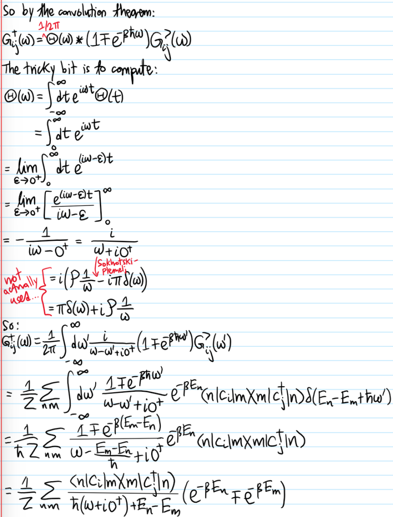
Problem: At a high level, what is the goal of classical hydrodynamics?
Solution: The program of classical hydrodynamics seeks to bridge the physics of a many-body system at different length scales. The idea is to start from microscopics (i.e. Newton’s laws) and derive mesoscopics (i.e. Boltzmann equation), and from there to derive macroscopics (i.e. Navier-Stokes equations). Of course, there is also a field of quantum hydrodynamics, but that’s for another day…
Problem: In light of the above, it is useful to start with Newton’s laws, but in their Hamiltonian formulation. In order to coarse grain from this microscopic description to a mesoscopic description, the natural way to achieve such a coarse graining is to construct (i.e. pull out of thin air!) a probability density function \(\rho(\textbf x_1,…,\textbf x_N,\textbf p_1,…,\textbf p_N,t)\) defined on the joint phase space \(\cong\textbf R^{6N}\) of the \(N\)-body system. Give a more precise interpretation to \(\rho\).
Solution: The precise interpretation is that \(\rho(\textbf x_1,…,\textbf x_N,\textbf p_1,…,\textbf p_N,t)d^3\textbf x_1…d^3\textbf x_Nd^3\textbf p_1…d^3\textbf p_N\) is the probability (purely due to classical ignorance) that the system of \(N\) (in general not necessarily identical) particles is, at some time \(t\), living within an infinitesimal volume \(d^3\textbf x_1…d^3\textbf x_Nd^3\textbf p_1…d^3\textbf p_N\) centered around the (micro)state \((\textbf x_1,…,\textbf x_N,\textbf p_1,…,\textbf p_N)\) in the joint phase space.
Problem: State the equation of motion obeyed by \(\rho\) (i.e. Liouville’s equation).
Solution: Remembering the intuition that \(\{\space\space,H\}\) implements an advective derivative on the joint phase space (the essence of Hamilton’s equations):
\[\left(\frac{D\rho}{Dt}\right)_H=0\Rightarrow\dot{\rho}+\{\rho,H\}=0\]
so probability flows incompressibly throughout phase space under \(H\).
Problem: From this joint probability density function \(\rho\), explain how to marginalize to obtain the single-particle probability density function \(\rho_1(\textbf x,\textbf p,t)\) for say “particle #\(1\)”.
Solution: Simply integrate away the \(6(N-1)\) degrees of freedom of the other \(N-1\) particles:
\[\rho_1(\textbf x,\textbf p,t)=\int d^3\textbf x_2…d^3\textbf x_Nd^3\textbf p_2…d^3\textbf p_N\rho(\textbf x,…\textbf x_N,\textbf p,…,\textbf p_N,t)\]
Thus, \(\rho_1(\textbf x,\textbf p,t)d^3\textbf x d^3\textbf p\) represents the probability (again due to classical ignorance) that “particle \(1\)” will, at some time \(t\), be found in the infinitesimal cell \(d^3\textbf xd^3\textbf p\) centered around the state \((\textbf x,\textbf p)\) in its (single-particle) phase space.
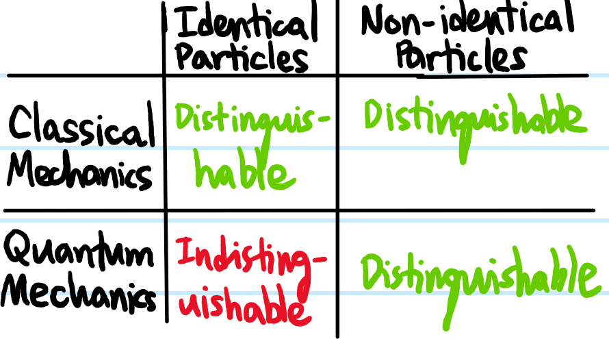
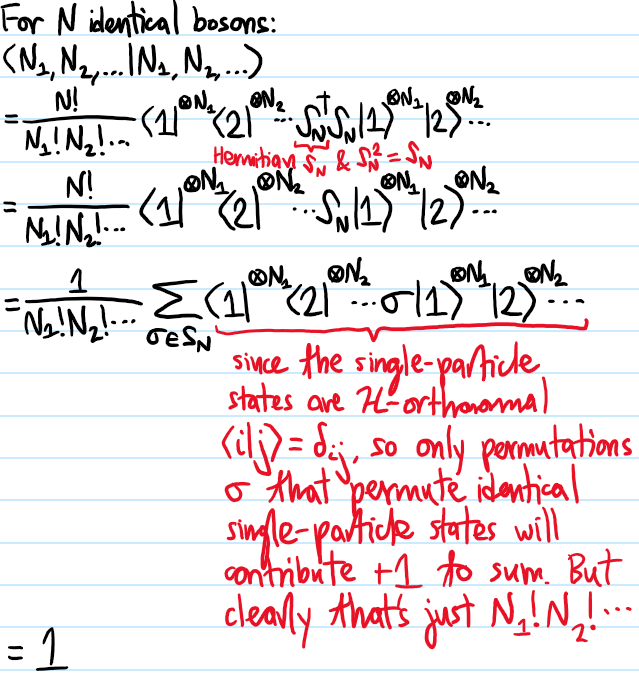
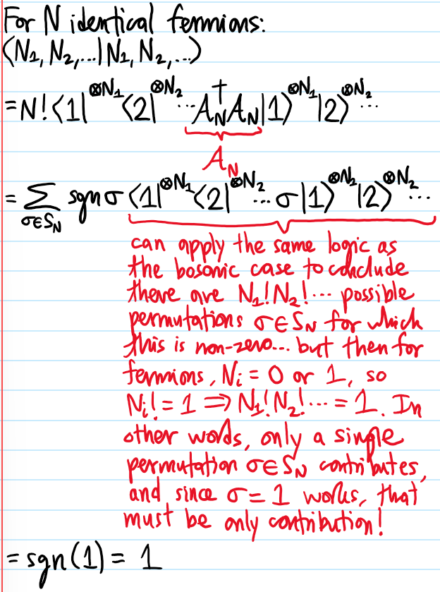
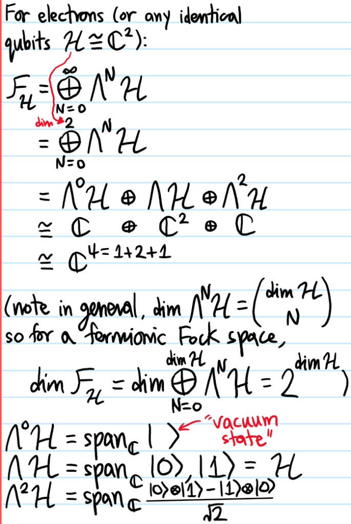
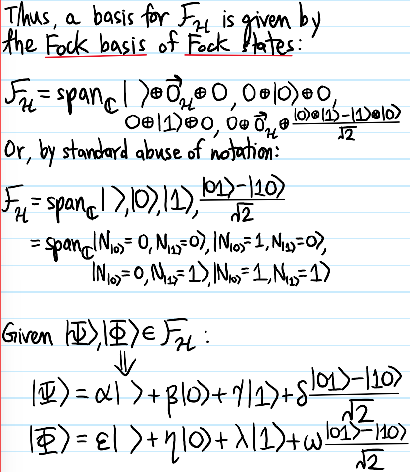
Problem: Henceforth suppose (as is often the case) that the \(N\) particles are identical. Explain what the best way is to exploit this additional assumption of indistinguishability.
Solution: Rather than working with \(\rho_1\), work with \(n_1:=N\rho_1\); this sort of like a classical analog of the quantum mechanical passage from first quantization (Slater permanent/determinants) to second quantization (occupation numbers) in many-body quantum mechanics of identical bosons/fermions.
Problem: Derive the analog of the Liouville equation for \(n_1(\textbf x,\textbf p,t)\) (a.k.a. the Boltzmann equation):
\[\left(\frac{Dn_1}{Dt}\right)_{H_1}=(\dot n_1)_c\]
where the collision integral source term \((\dot n_1)_c\) is given by:
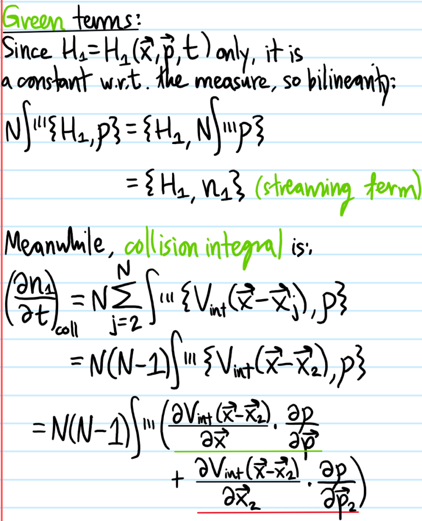
\[(\dot n_1)_c=\int d^3\textbf x_2 d^3\textbf p_2\frac{\partial V_{\text{int}}(\textbf x-\textbf x_2)}{\partial\textbf x}\cdot\frac{\partial n_2}{\partial\textbf p}\]
where \(n_2:=N(N-1)\int d^3\textbf x_3…d^3\textbf x_Nd^3\textbf p_3…d^3\textbf p_N\rho\). Specify the actual physics by assuming the Hamiltonian \(H\) has the generic dispersion:
\[H=\sum_{i=1}^NH_i+\sum_{1\leq i<j\leq N}V_{\text{int}}(\textbf x_i-\textbf x_j)\]
where \(H_i:=\frac{|\textbf p_i|^2}{2m}+V_{\text{ext}}(\textbf x_i)\), and in general for \(i=1\) one writes \(\textbf x:=\textbf x_1\) and \(\textbf p:=\textbf p_1\).
Solution: Using the Liouville equation for \(\rho\) as a springboard, the Boltzmann equation for \(n_1\) looks like:
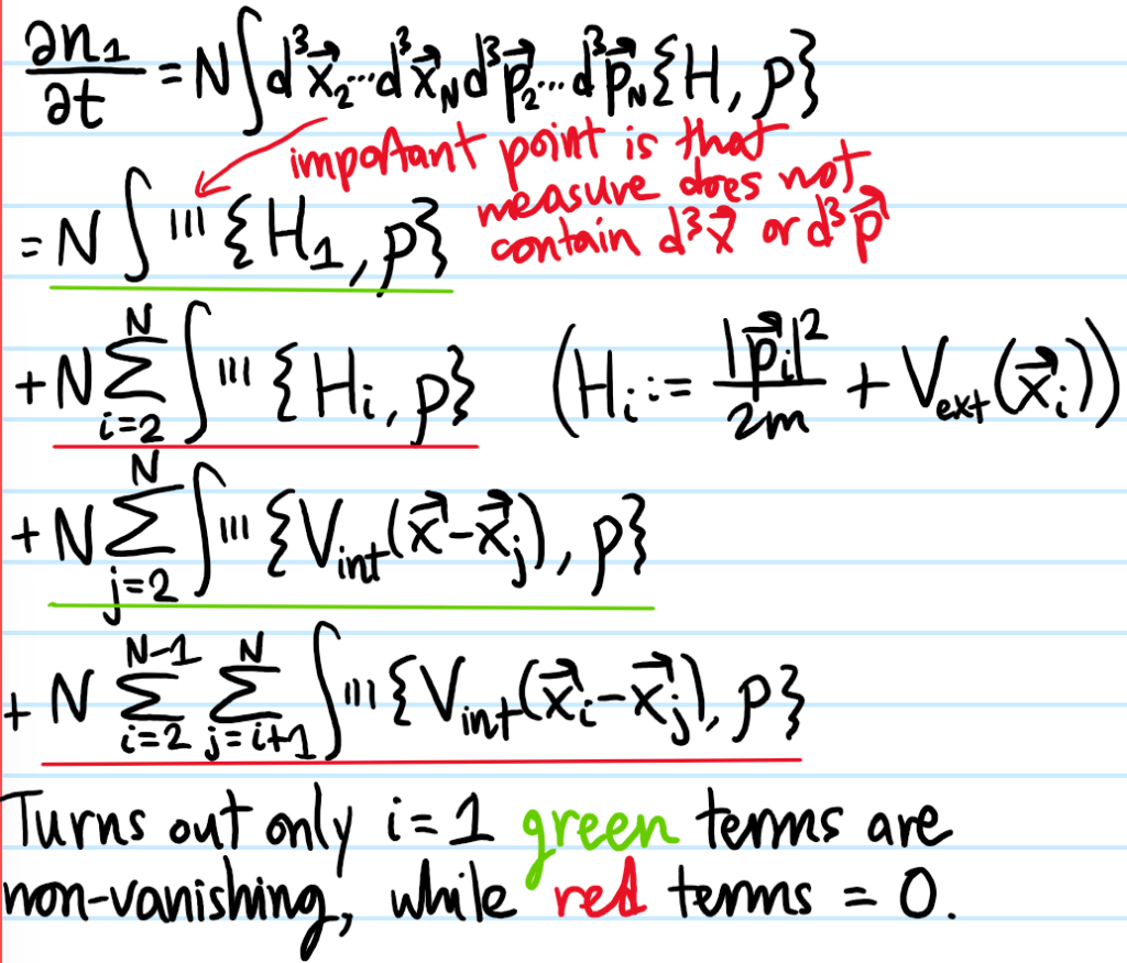


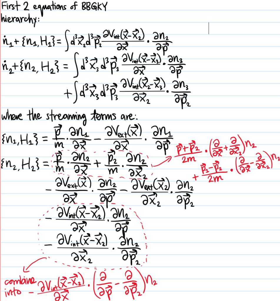
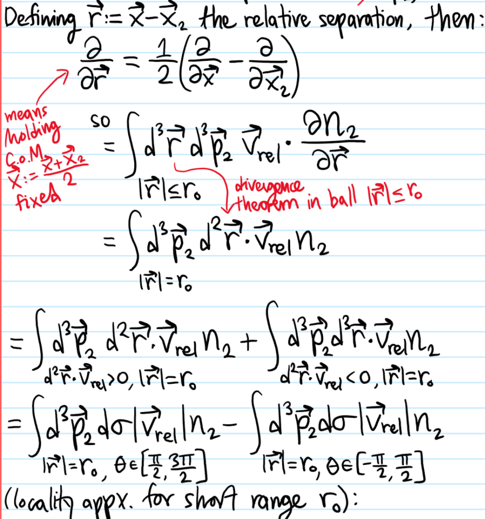
Problem: In writing the Boltzmann equation for \(\dot n_1\) above, it was natural to introduce the quantity \(n_2(\textbf x,\textbf x_2,\textbf p,\textbf p_2,t)\). If one were to repeat the above derivation, namely evaluate \(\dot n_2\) using Liouville’s equation for \(\dot{\rho}\) again, what result would one find?
Solution: One would get a result most naturally expressed in terms of a quantity \(n_3:=N(N-1)(N-2)\int d^3\textbf x_4…d^3\textbf x_Nd^3\textbf p_4…d^3\textbf p_N\rho\), and so forth. This ladder of \(N\) equations forms the BBGKY hierarchy:
\[\frac{\partial n_k}{\partial t}=\{H_k,n_k\}+\sum_{i=1}^{k}\int d^3\textbf x_{k+1}d^3\textbf p_{k+1}\frac{\partial V_{\text{int}}(\textbf x_i-\textbf x_{k+1})}{\partial\textbf x_i}\cdot\frac{\partial n_{k+1}}{\partial\textbf p_i}\]
where the \(k\)-body distribution function is:
\[n_k(\textbf x_1,…\textbf x_k,\textbf p_1,…,\textbf p_k,t)=\frac{N!}{(N-k)!}\int d^3\textbf x_{k+1}…d^3\textbf x_Nd^3\textbf p_{k+1}…d^3\textbf p_N n(\textbf x_1,…,\textbf x_N,\textbf p_1,…,\textbf p_N,t)\]
and \(k\)-particle Hamiltonian \(H_k\) including both \(V_{\text{ext}}\) and interactions \(V_{\text{int}}\) among the first \(k\) particles but ignores interactions with the other \(N-k\) particles:
\[H_k=\sum_{i=1}^{k}\left(\frac{|\textbf p_i|^2}{2m}+V_{\text{ext}}(\textbf x_i)\right)+\sum_{1\leq i<j\leq k}V_{\text{int}}(\textbf x_i-\textbf x_j)\]
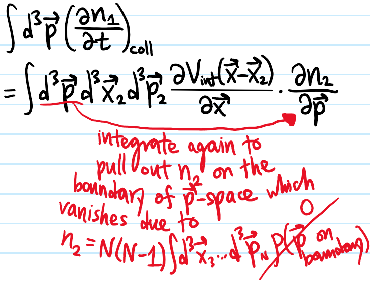
Problem: Define the real space number density \(n(\textbf x,t)\) in terms of \(n_1(\textbf x,\textbf p,t)\) and show that it’s not influenced by the collision integral.
Solution: One has \(n(\textbf x,t):=\int d^3\textbf p n_1(\textbf x,\textbf p,t)\). So:
\[\dot n=\int d^3\textbf p\{H_1,n_1\}+\int d^3\textbf p(\dot n_1)_c\]
but the \(d^3\textbf p\)-integral over the collision integral vanishes for the same kind of reasons as above:
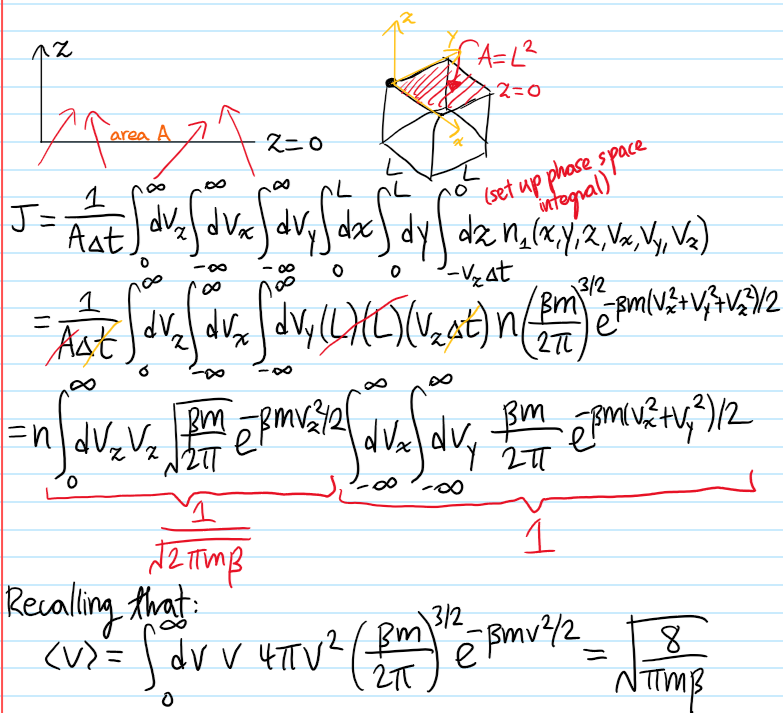
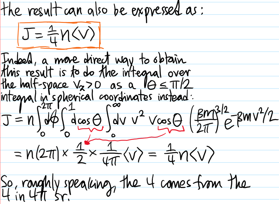
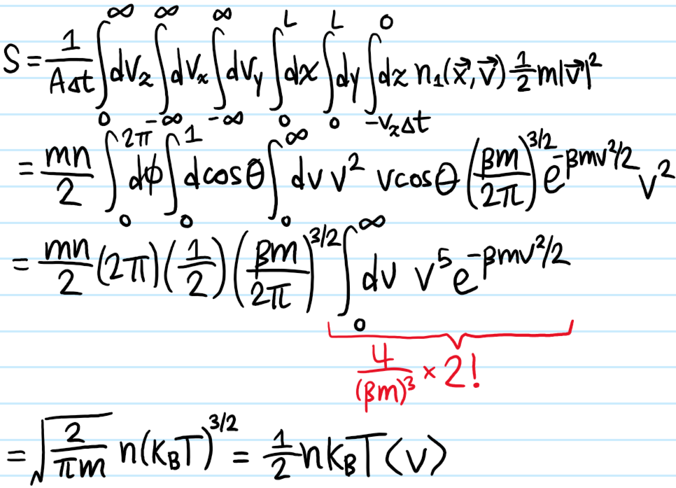
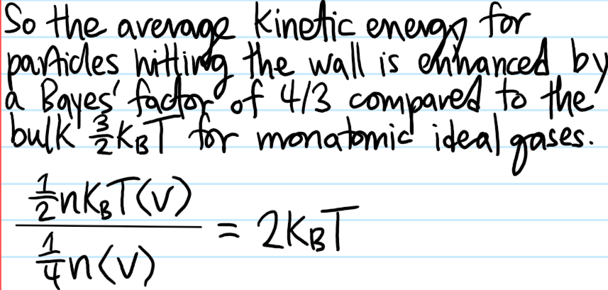
Problem: What about for the momentum space number density \(n(\textbf p,t):=\int d^3\textbf x n_1(\textbf x,\textbf p,t)\)? What about for the real space momentum density \(\int d^3\textbf p\textbf pn_1\) or the real space kinetic energy density \(\int d^3\textbf p|\textbf p|^2n_1/2m\)?
Solution: In all these cases, the collision integral will contribute!
Problem: Show that a classical elastic \(2\)-body collision between equal-mass particles implies (though is not equivalent to) an \(O(3)\) isometry on their relative momentum.
Solution: Conservation of momentum:
\[\textbf p+\textbf p_2=\textbf p’_1+\textbf p’_2\]
\[|\textbf p+\textbf p_2|^2=|\textbf p’_1+\textbf p’_2|^2\]
\[|\textbf p|^2+|\textbf p_2|^2+2\textbf p\cdot\textbf p_2=|\textbf p’_1|^2+|\textbf p’_2|^2+2\textbf p’_1\cdot\textbf p’_2\]
Using conservation of kinetic energy for equal masses \(|\textbf p|^2+|\textbf p_2|^2=|\textbf p’_1|^2+|\textbf p’_2|^2\):
\[\textbf p\cdot\textbf p_2=\textbf p’_1\cdot\textbf p’_2\]
So:
\[|\textbf p|^2+|\textbf p_2|^2-2\textbf p\cdot\textbf p_2=|\textbf p’_1|^2+|\textbf p’_2|^2-2\textbf p’_1\cdot\textbf p’_2\]
\[|\textbf p-\textbf p_2|^2=|\textbf p’_1-\textbf p’_2|^2\]
\[|\textbf p-\textbf p_2|=|\textbf p’_1-\textbf p’_2|\]
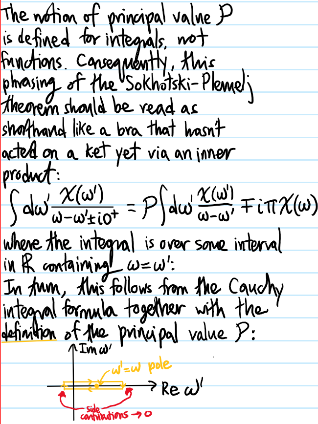
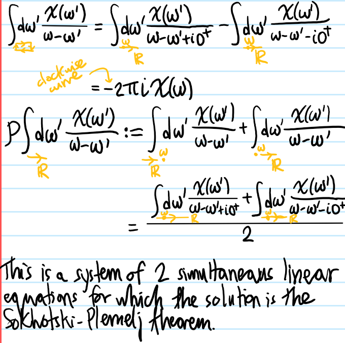
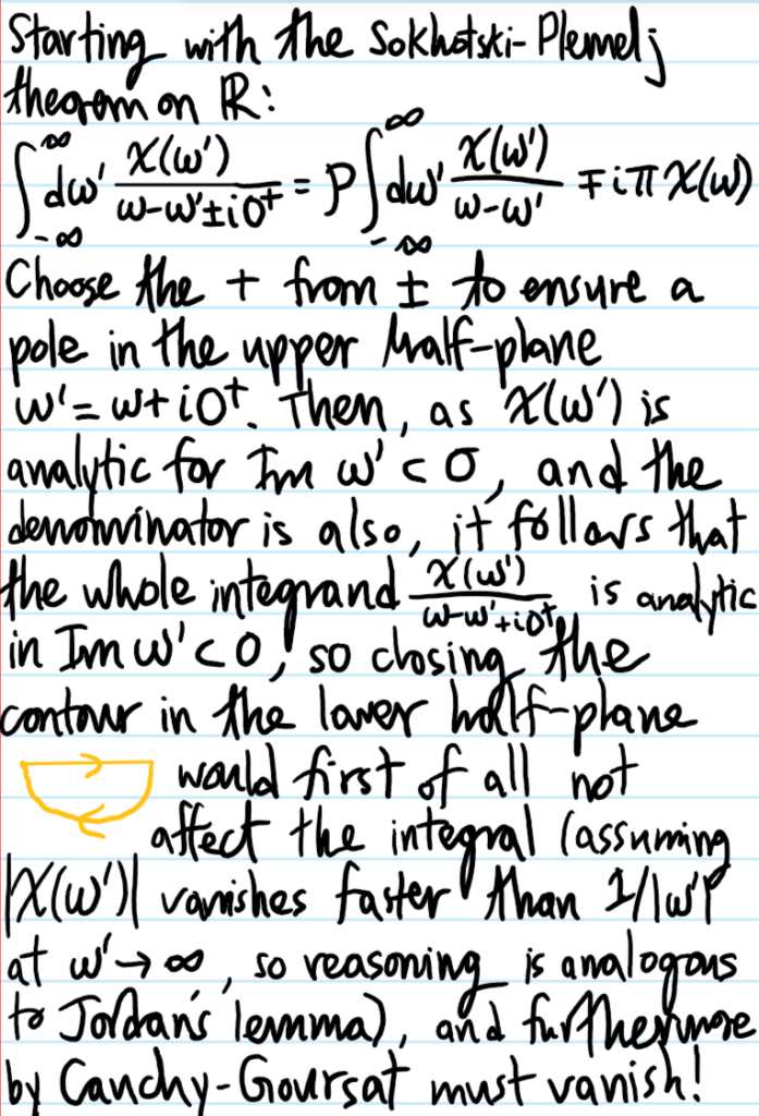
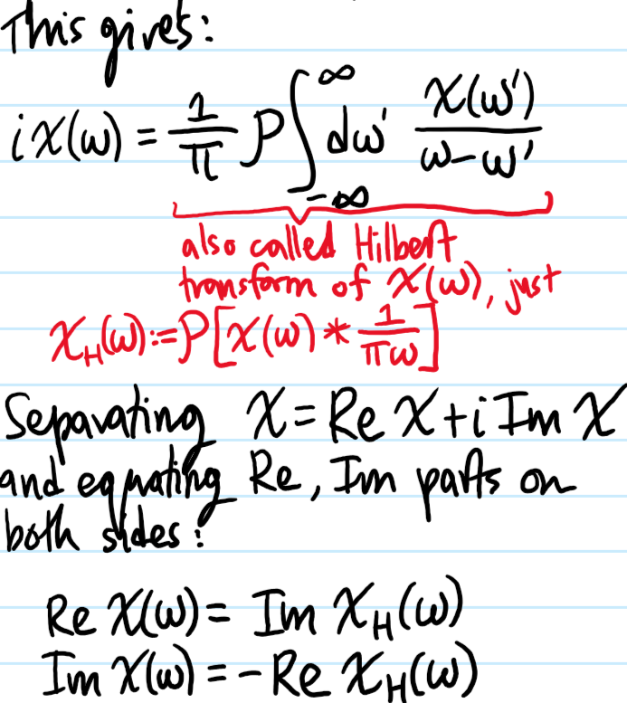
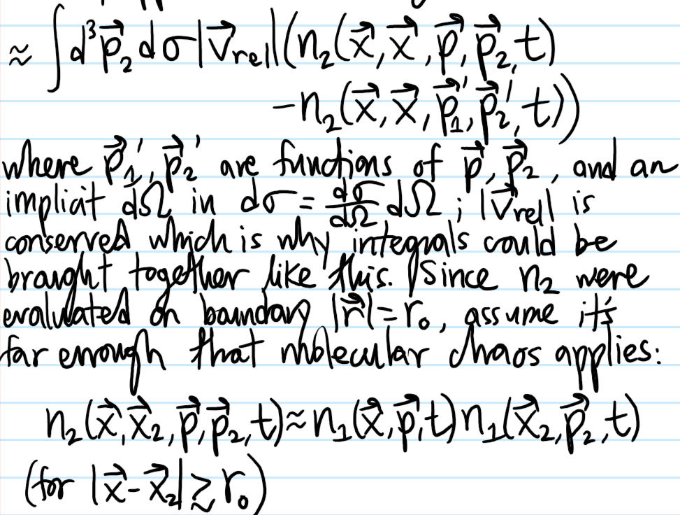
Problem: Strictly speaking, the above is actually a precursor to the actual Boltzmann equation. So then, how does the actual Boltzmann equation arise from the BBGKY hierarchy? Make sure to clearly identify all assumptions.
Solution:
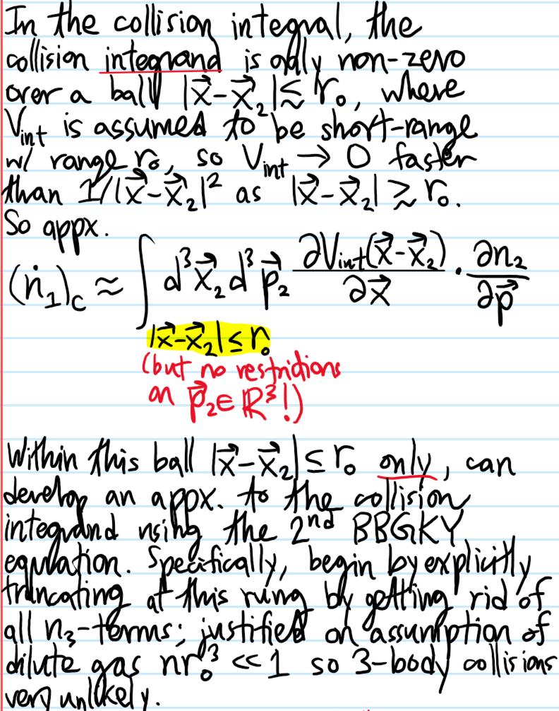
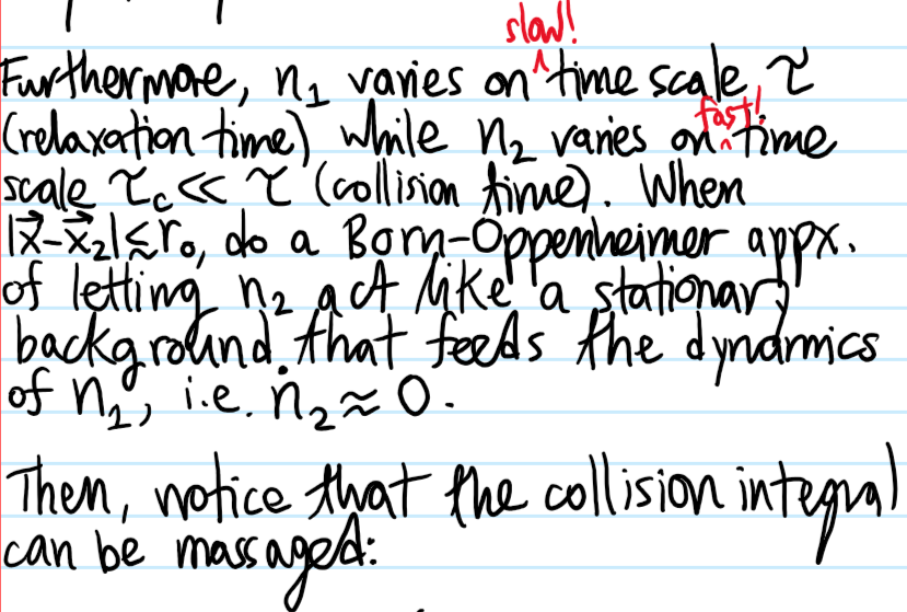
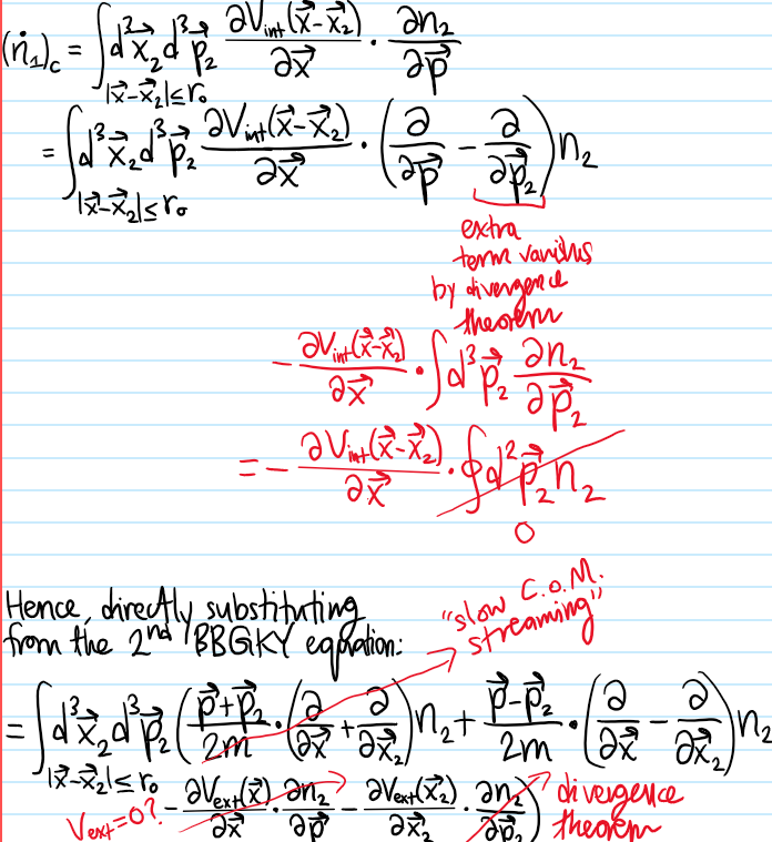
One thus obtains the actual Boltzmann (integrodifferential!) equation for \(n_1\), which still asserts that:
\[\left(\frac{Dn_1}{Dt}\right)_{H_1}=(\dot n_1)_c\]
but now with the collision integral expressed solely in terms of \(n_1\):
\[(\dot n_1)_c=\int d^3\textbf p_2d\sigma|\textbf v_{\text{rel}}|(n_1(\textbf x,\textbf p’_1,t)n_1(\textbf x,\textbf p’_2,t)-n_1(\textbf x,\textbf p,t)n_1(\textbf x,\textbf p_2,t))\]
where \(|\textbf v_{\text{rel}}|:=|\textbf p-\textbf p_2|/m=|\textbf p’_1-\textbf p’_2|/m\) is conserved, and in practice one should compute the differential cross-section \(d\sigma=\frac{d\sigma}{d\Omega}d\Omega\) from the interaction potential \(V_{\text{int}}\), and both post-collision momenta \(\textbf p’_1,\textbf p’_2\) are determined from \(\textbf p_1,\textbf p_2\) and \(d\Omega\) by elasticity.
On dimensional analysis grounds, the way to read the collision integral is as follows:
\[(\dot n_1)_c=\text{momentum}^3\times\frac{\text{volume}}{\text{time}}\frac{1}{\text{volume}^2\text{momentum}^6}=\frac{1/(\text{volume}\times\text{momentum}^3)}{\text{time}}\]
Problem: Elaborate more on the molecular chaos assumption and how it resolves Loschmidt’s paradox concerning the arrow of time \(t\).
Solution: The molecular chaos assumption essentially is the assertion that the pre-collision velocities are uncorrelated. The prefix “pre” is what breaks time reversal symmetry, despite the underlying Hamiltonian mechanics being time reversible.
Problem: Prove that the quantity:
\[-\frac{S(t)}{k_B}:=\int d^3\textbf xd^3\textbf pn_1\ln n_1\]
never increases with time \(t\).
Solution: Taking the time derivative:
\[-\frac{\dot S}{k_B}=\int d^3\textbf xd^3\textbf p\dot n_1(1+\ln n_1)\]
but \(N=\int d^3\textbf xd^3\textbf pn_1\) is conserved so that \(\dot N=\int d^3\textbf xd^3\textbf p\dot n_1=0\). Then of course, one should invoke Boltzmann’s equation:
\[=-\int d^3\textbf xd^3\textbf p\left(\frac{\textbf p}{m}\cdot\frac{\partial n_1}{\partial\textbf x}-\frac{\partial V_{\text{ext}}(\textbf x)}{\partial\textbf x}\cdot\frac{\partial n_1}{\partial\textbf p}\right)\ln n_1\]
\[+\int d^3\textbf xd^3\textbf pd^3\textbf p_2d\sigma|\textbf v_{\text{rel}}|(n_1(\textbf x,\textbf p’_1,t)n_1(\textbf x,\textbf p’_2,t)-n_1(\textbf x,\textbf p,t)n_1(\textbf x,\textbf p_2,t))\ln n_1(\textbf x,\textbf p,t)\]
Now integrate the first row above by parts:
\[\int d^3\textbf xd^3\textbf p\left(\frac{\textbf p}{m}\cdot\frac{\partial n_1}{\partial\textbf x}-\frac{\partial V_{\text{ext}}(\textbf x)}{\partial\textbf x}\cdot\frac{\partial n_1}{\partial\textbf p}\right)\ln n_1\]
\[=\int d^3\textbf p\frac{\textbf p}{m}\cdot\int d^3\textbf x\frac{\partial n_1}{\partial\textbf x}\ln n_1-\int d^3\textbf x\frac{\partial V_{\text{ext}}(\textbf x)}{\partial\textbf x}\cdot\int d^3\textbf p\frac{\partial n_1}{\partial\textbf p}\ln n_1\]
where:
\[\int d^3\textbf x\frac{\partial n_1}{\partial\textbf x}\ln n_1=\oint d^2\textbf x n_1\ln n_1-\int d^3\textbf x\frac{\partial n_1}{\partial\textbf x}=\oint d^2\textbf x n_1(\ln n_1-1)=0\]
and similarly for the other term.
To complete the proof, one just has to show that the collision integral term is \(\leq 0\). This is slightly more delicate, requiring one to first symmetrize between the particles \(\textbf p\Leftrightarrow\textbf p_2\) to obtain:
\[\frac{1}{2}\int d^3\textbf xd^3\textbf pd^3\textbf p_2d\sigma|\textbf v_{\text{rel}}|(n_1(\textbf x,\textbf p’_1,t)n_1(\textbf x,\textbf p’_2,t)-n_1(\textbf x,\textbf p,t)n_1(\textbf x,\textbf p_2,t))(\ln n_1(\textbf x,\textbf p,t)+\ln n_1(\textbf x,\textbf p_2,t))\]
and then further symmetrizing between past and future \((\textbf p,\textbf p_2)\Leftrightarrow(\textbf p’_1,\textbf p’_2)\) to get:
\[-\frac{1}{4}\int d^3\textbf xd^3\textbf pd^3\textbf p_2d\sigma|\textbf v_{\text{rel}}|(x-y)(\ln x-\ln y)\]
where \(x:=n_1(\textbf x,\textbf p’_1,t)n_1(\textbf x,\textbf p’_2,t)\) and \(y:=n_1(\textbf x,\textbf p,t)n_1(\textbf x,\textbf p_2,t)\). But the integrand is positive for all \(x,y>0\):
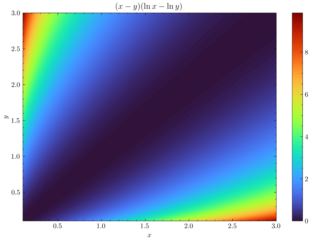
and “Boltzmann’s \(H\)-theorem” is proven.
Problem: A given single-particle phase space number density distribution \(n_1(\textbf x,\textbf p,t)\) is said to be in detailed balance iff for all locations \(\textbf x\in\textbf R^3\) and momenta \(\textbf p,\textbf p_2,\textbf p’_1,\textbf p’_2\in\textbf R^3\) obeying \(\textbf p+\textbf p_2=\textbf p’_1+\textbf p’_2\) and \(|\textbf p|^2+|\textbf p_2|^2=|\textbf p’_1|^2+|\textbf p’_2|^2\) (i.e. elastic collisions), one has the identity:
\[n_1(\textbf x,\textbf p,t)n_1(\textbf x,\textbf p_2,t)=n_1(\textbf x,\textbf p’_1,t)n_1(\textbf x,\textbf p’_2,t)\]
With this definition, show that the following statements are logically equivalent:
- \(n_1\) is in detailed balance.
- Collisions produce no entropy.
- \(\ln n_1\) is a collisional invariant, i.e.
\[\ln n_1(\textbf x,\textbf p,t)+\ln n_1(\textbf x,\textbf p_2,t)=\ln n_1(\textbf x,\textbf p’_1,t)+\ln n_1(\textbf x,\textbf p’_2,t)\]
- \(n_1(\textbf x,\textbf p,t)=n(\beta/2\pi m)^{3/2}\exp(-\beta|\textbf p-m\textbf v|^2/2m)\) for some functions \(n(\textbf x,t),\textbf v(\textbf x,t),\beta(\textbf x,t)\) (this is also called the Maxwell-Boltzmann distribution or, more profoundly, local equilibrium, which reduces to the usual thermodynamic case of global equilibrium iff \(n, \textbf v, \beta\) are constant parameters rather than spatiotemporally varying).
Solution: First, assume that \(n_1\) is in detailed balance (aside: the adjective detailed in this context is roughly synonymous with the adjective pairwise; it emphasizes that the balance doesn’t just come from e.g. \(5\) people standing in a circle and each person passing an apple to the person on their left, but that if Alice gives Bob \(3\) apples then Bob will also give Alice \(3\) apples). Then clearly, this is just the \(y=x\) diagonal in the graph! Thus, \(\dot S=0\). #2 is also clearly seen to imply #1 thanks to Boltzmann’s \(H\)-theorem. It is also trivial to check #1 is equivalent to #3.
In addition, \(n_1\) is in detailed balance if and only if \(\ln n_1\) is a collisional invariant. Finally, #3 can be argued to imply #4 by the fact that, since \(\ln n_1\) is a collisional invariant, it must be a linear combination of other collisional invariants \(\ln n_1\in\text{span}_{\textbf R}(1,\textbf p,|\textbf p|^2\}\), so there exist parameters \(\mu, \beta, \textbf v\) such that:
\[\ln n_1(\textbf x,\textbf p,t)=\beta(\mu+\textbf v\cdot\textbf p+|\textbf p|^2/2m)\]
\[n_1(\textbf x,\textbf p,t)=ze^{\beta(|\textbf p|^2/2m+\textbf v\cdot\textbf p)}\]
where the “fugacity” \(z:=e^{\beta\mu}\) is fixed by the normalization \(n=\int d^3\textbf pn_1\), and results in the form stated. The converse is of course trivial to show.