Problem: Distinguish between the terms “intrinsic semiconductor” and “extrinsic semiconductor“.
Solution: An intrinsic semiconductor is pretty much what it sounds like, i.e. a “pure” semiconductor material like \(\text{Si}\) that is undoped with any impurity dopants. An extrinsic semiconductor is then basically the negation of an intrinsic semiconductor, i.e. one which is doped with impurity dopants, although conceptually one can think of it as being doped with charge carriers (either holes \(h^+\) in a \(p\)-type extrinsic semiconductor or electrons \(e^-\) in an \(n\)-type extrinsic semiconductor).
Problem: In the phrases \(p\)-type semiconductor and \(n\)-type semiconductor, what do the \(p\) and \(n\) represent?
Solution: In both cases, the extrinsic semiconductor (isolated from anything else) is neutral, even when doped. Rather, the \(p\) and \(n\) refer to the majoritymobile/free charge carriers in the corresponding semiconductor; i.e. holes in the valence band and electrons in the conduction band respectively.
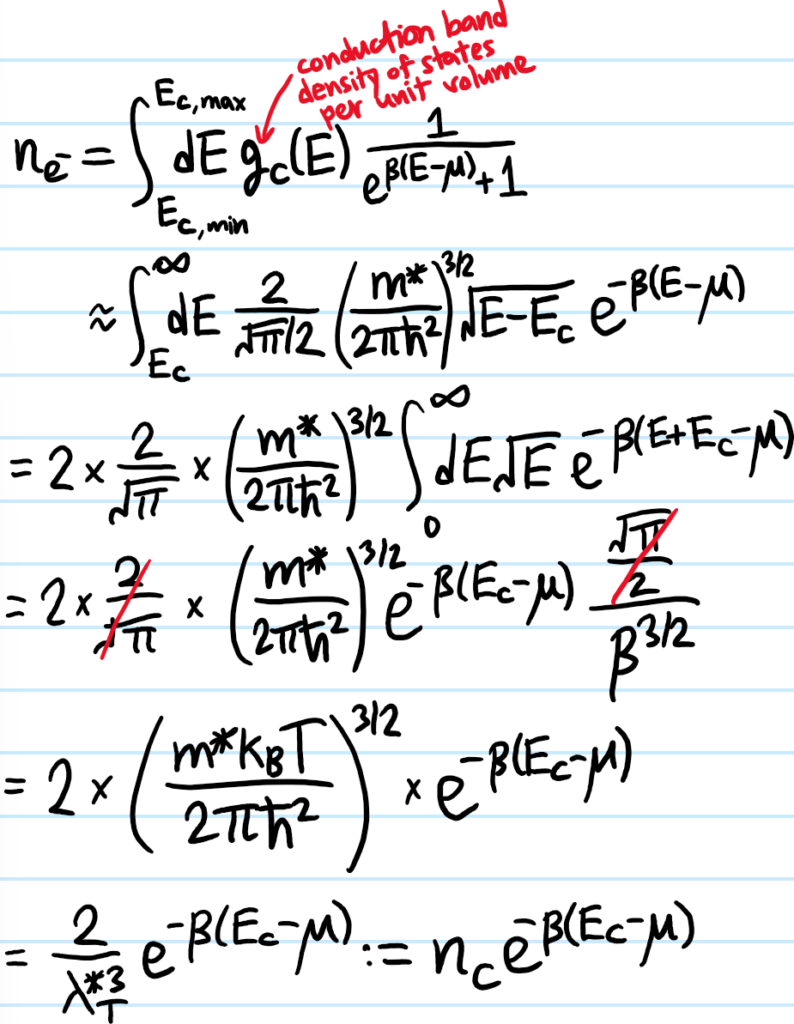
Problem: Show that the equilibrium number density \(n_{e^-}\) of mobile conduction electrons (i.e. not including the immobile core/valence electrons) thermally excited into the conduction band at temperature \(T\) is exponentially related to the gap \(E_C-\mu\) between the energy \(E_C\) at the base of the conduction band and the Fermi level \(\mu\):
\[n_{e^-}=n_Ce^{-\beta(E_C-\mu)}\]
where the so-called effective density of states:
\[n_C:=\frac{2g_v}{\lambda^{*3}_T}\]
is \(\approx\) the number density of available conduction band states at temperature \(T\) (here \(g_v\) is the valley degeneracy and \(\lambda^{*3}_T\) is the thermal de Broglie wavelength with respect to the electron’s effective mass \(m^*\)).
Solution: To clarify some of the approximations used in that line with the \(\approx\), the upper bound on the conduction band \(E_{C,\text{max}}\to\infty\) can be safely taken to infinity because of the exponential suppression of the integrand by the Fermi-Dirac distribution for \(E\gg\mu\) (in fact, using Fermi-Dirac statistics in the first place assumes the electrons interact solely through Pauli blocking). In addition, the density of states \(g_C(E)\) is approximated by that of a free particle in the neighbourhood of the conduction band valley (with the usual \(\sqrt{E}\mapsto \sqrt{E-E_C}\) because \(g_C(E)=0\) in the \(E\in[E_V,E_C]\) band gap) and with \(m\mapsto m^*\) to reflect the local curvature of the conduction band which is inherited from the strength of the lattice’s periodic potential. Finally, to strengthen the earlier claim that \(E\gg\mu\), indeed, \(E\geq E_C\) is the range of the integral, and so a sufficient condition for \(E\gg\mu\) is \(E_C\gg\mu\) (in practice a few \(k_BT\) is sufficient). This is assumed to be the case, and constitutes the assumption of a non-degenerate semiconductor (cf. non-degenerate Fermi gas). In this case, the Fermi-Dirac distribution boils down to just its “Boltzmann tail” \(\frac{1}{e^{\beta(E-\mu)}+1}\approx e^{-\beta(E-\mu)}\):
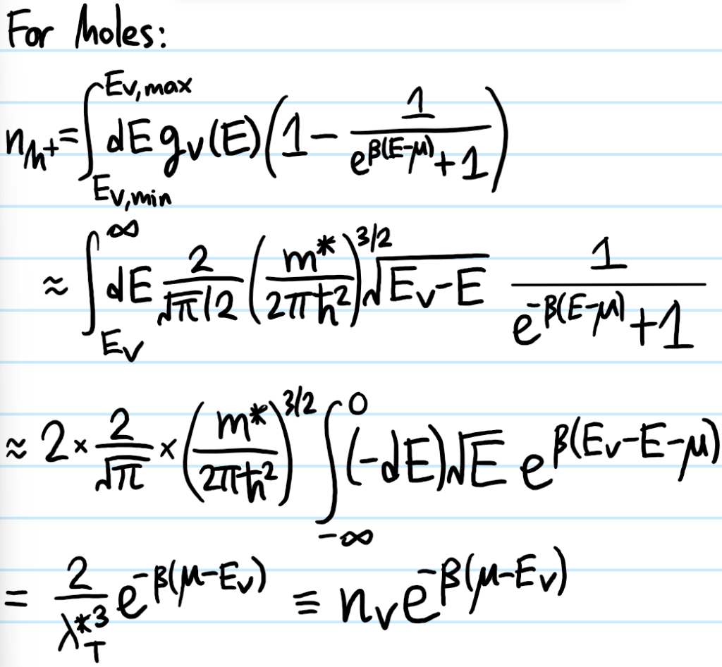
Problem: Repeat the above problem for holes to derive an analogous result for the equilibrium number density \(n_{h^+}\) of free conduction holes excited into the valence band at temperature \(T\):
\[n_{h^+}=n_Ve^{-\beta(\mu-E_V)}\]
where \(n_V\) is almost the same as \(n_C\) except that it’s derived from the effective mass \(m^*\) of the holes at the top of the valence band.
Solution: A few comments: if \(f(E)\) is the Fermi-Dirac distribution for electrons, then by the very definition of a hole as a vacancy/absence of an electron, the analog of the Fermi-Dirac distribution for holes (which can be considered fermionic quasiparticles) is \(1-f(E)\). In addition, a hole is considered to have more energy when it goes “downward” on a typical band diagram where the vertical axis \(E\) is really referring to the electron’s energy. This explains the counterintuitive limits on the integral:
Problem: If an intrinsic semiconductor is doped with impurity dopants to create an extrinsic semiconductor, say with a number density \(n_{d^+}\) of cationized donor dopants and \(n_{a^-}\) of anionized acceptor dopants, what constraint does charge neutrality of the semiconductor impose among the concentrations \(n_{e^-},n_{h^+},n_{d^+},n_{a^-}\)?
Solution:
\[-en_{e^-}+en_{h^+}+en_{d^+}-en_{a^-}=0\]
\[n_{h^+}+n_{d^+}=n_{e^-}+n_{a^-}\]
Conceptually, for every electron excited into the conduction band, the corresponding donor atom now becomes cationized; similarly, every hole excited into a valence band is really an acceptor atom anionizing as it accepts an electron from the valence band, so in the equation, it is conceptually meaningful to pair up \((n_{e^-},n_{d^+})\) and \((n_{h^+},n_{a^-})\). Note however this is not saying that they are equal; though they approach becoming equal the more heavily one dopes.
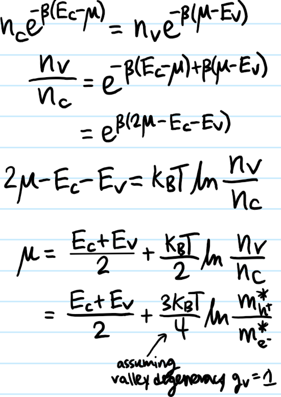
Problem: Show that, in an intrinsic semiconductor, the Fermi level \(\mu\) lies almost (but not exactly) at the midpoint \(\frac{E_V+E_C}{2}\) of the band gap.
Solution: An intrinsic semiconductor is undoped so \(n_{D^+}=n_{A^-}=0\). This implies from the charge neutrality argument above that \(n_{e^-}=n_{h^+}\) (i.e. every electron excited into the conduction band leaves a hole in the valence band). The rest of the argument is then just plugging in the earlier equilibrium free charge carrier concentrations and algebra:
In what follows, it will be useful to call this particular value of \(\mu\) the intrinsic Fermi level \(\mu_i\) since it is the Fermi level of an intrinsic semiconductor, prior to any extrinsic doping.
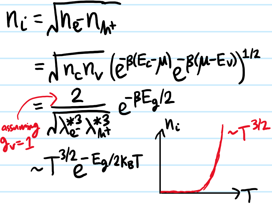
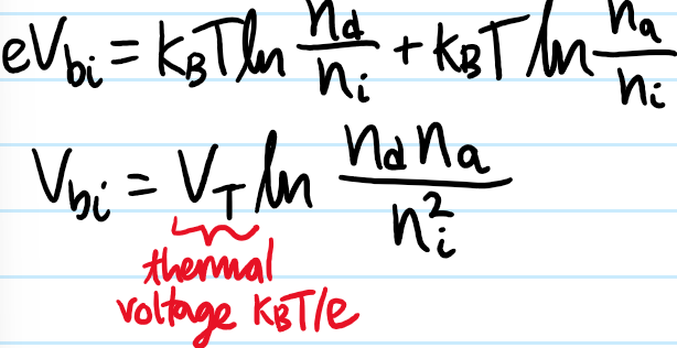
Problem:Define the intrinsic charge carrier concentration by \(n_i:=n_{e^-}=n_{h^+}\) for an intrinsic semiconductor, hence one has the so-called law of mass action \(n_{e^-}n_{h^+}=n_i^2\) (i.e. \(n_i^2\) is just a \(T\)-dependent equilibrium constant for the dissociation reaction \(0\to e^-+h^+\)). Show that the precise \(T\)-dependence of \(n_i\) is given by:
\[n_i\sim T^{3/2}e^{-E_g/2k_BT}\]
where the band gap \(E_g:=E_C-E_V\) (this result is sometimes also presented as \(n_i=n_Se^{-\beta E_g/2}\) where \(n_S:=\sqrt{n_Cn_V}\) is the geometric mean of the effective densities of states of the conduction and valence bands).
Solution:
Problem: Keeping tempertature \(T\) fixed, consider \(n\)-type doping an intrinsic semiconductor with donor dopants, thus creating an \(n\)-type extrinsic semiconductor. The effect of this will be to raise the Fermi level from the intrinsic Fermi level \(\mu_i\) (appx. in the middle of the band gap as shown earlier) to a new value \(\mu\) much closer to the base of the conduction band \(E_C\). Show that the precise amount of this raising can be quantified by:
\[\mu-\mu_i=k_BT\ln\frac{n_d}{n_i}\]
where \(n_d\) is the (directly manipulable!) concentration of donor dopants doped into the intrinsic semiconductor, stating the \(2\) key assumptions underlying this.
(note, an analogous line of reasoning for a \(p\)-type semiconductor shows that the Fermi level is lowered by an amount:
\[\mu_i-\mu=k_BT\ln\frac{n_a}{n_i}\]
where \(n_a\) is the (also directly manipulable) concentration of acceptor dopants).
Solution: At equilibrium, one has for an intrinsic semiconductor:
\[n_i=n_Ce^{-\beta(E_C-\mu_i)}\]
and for an \(n\)-type doped extrinsic semiconductor:
\[n_{e^-}=n_Ce^{-\beta(E_C-\mu)}\]
Taking the ratio yields:
\[\mu-\mu_i=k_BT\ln\frac{n_{e^-}}{n_i}\]
At this point, the goal is to justify why \(n_{e^-}\approx n_{d}\). This proceeds in \(2\) stages.
First, justify that \(n_{e^-}\approx n_{d}^+\), the concentration of cationized donor dopants. This follows by setting \(n_{a^+}=0\) in the earlier charge neutrality constraint (since there are no acceptor dopants added \(n_a=0\Rightarrow n_{a^+}=0\)) and using the law of mass action to replace \(n_{h^+}=n_i^2/n_{e^-}\), obtaining a quadratic equation for \(n_{e^-}\) whose physical solution is:
And at this point, one assumes that the semiconductor is fairly heavily doped, in particular \(n_D\gg n_i\) (typical values in \(\text{Si}\) are \(n_D\sim 10^{16}\text{ cm}^{-3}\) while \(n_i\sim 10^{10}\text{ cm}^{-3}\)). This allows one to approximate \(n_{e^-}\approx n_{d^+}\).
2. Then, to justify why \(n_{d^+}\approx n_d\), one has to assume that the donor dopants are shallow in the sense that the binding energy of their extra valence electron is comparable to \(k_BT\), and so it is easily excited into the conduction band. In other words, assume that almost complete cationization of donor dopants. This is just the statement that \(n_{d^+}\approx n_d\), as desired.
Problem: In what regime is the non-degenerate semiconductor approximation valid?
Solution: For an \(n\)-type extrinsic semiconductor, a rule of thumb is that the Fermi level cannot rise to within \(2k_BT\) of the base of the conduction band \(E_C\):
\[E_c-\mu\geq 2k_BT\]
Inserting \(n_d=n_Ce^{-\beta (E_C-\mu)}\) (where the approximation \(n_{e^-}\approx n_d\) has been employed), one arrives at the rule of thumb that the donor dopant concentration cannot exceed:
\[n_d\leq e^{-2}n_C\approx 0.14 n_C\]
Similarly, for \(p\)-type doping, the acceptor dopant concentration cannot exceed:
\[n_a\leq 0.14n_V\]
(the more important takeaway here is not the exact numerical prefactors, but the fact that the Fermi level should stay a few \(k_BT\) away from \(E_C\) or \(E_V\) for the semiconductor to be considered non-degenerate; indeed these estimates came from using the Boltzmann formula that was derived from this assumption, so it should be taken with a grain of salt as one is using a theory to predict its own demise).
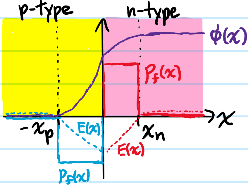
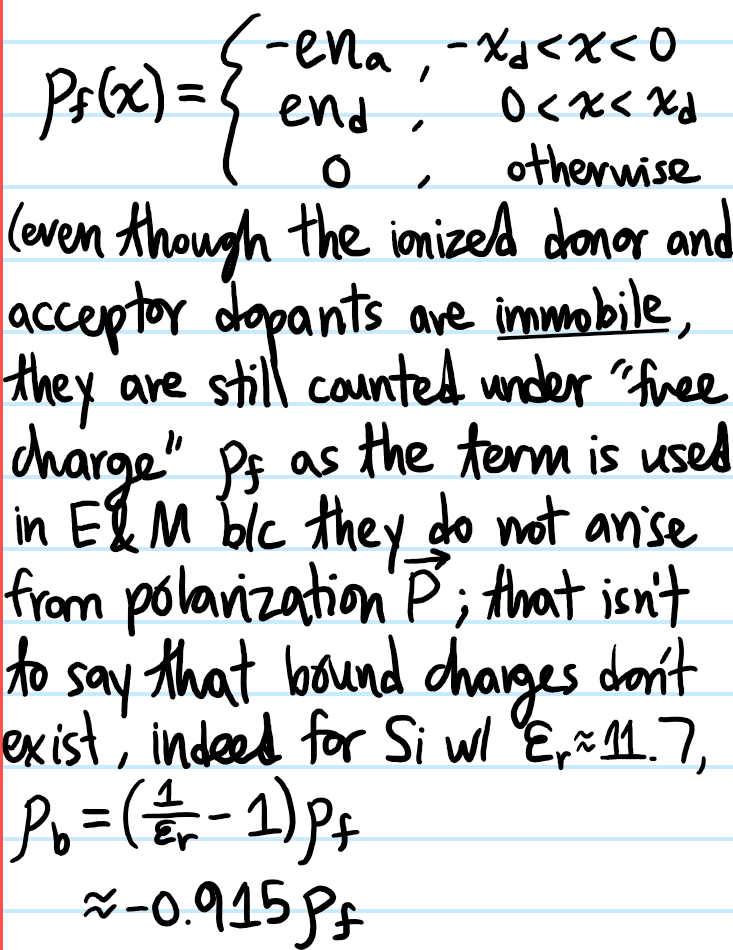
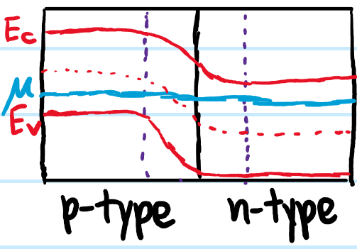
Problem: A \(p\)-\(n\) junction is formed by putting a \(p\)-type extrinsic semiconductor in contact with an \(n\)-type extrinsic semiconductor. Starting from a simple “top-hat” distribution of the free charge density \(\rho_f(x)\) in the depletion region \(-x_p<x<x_n\), sketch \(\rho_f(x)\), \(E(x)\) and \(\phi(x)\).
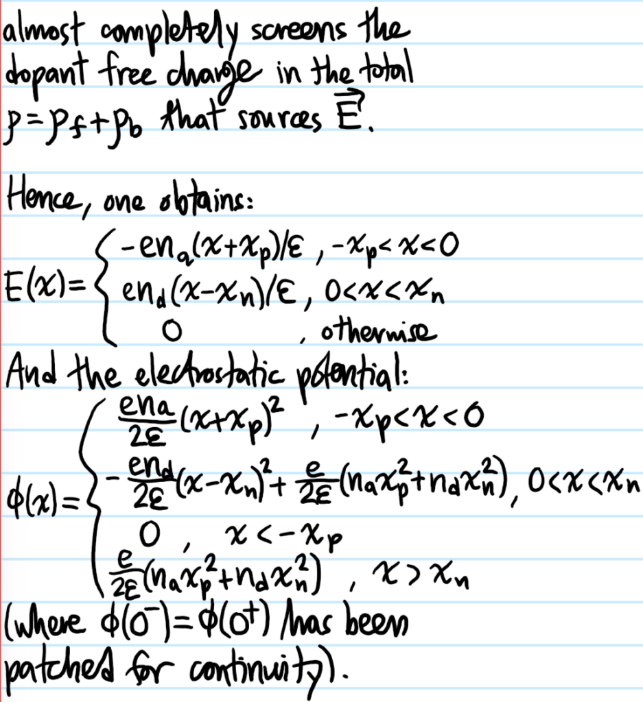
Solution: Assuming an abrupt junction and sharp cutoff for the depletion region at \(x_p, x_n\) respectively, one has:
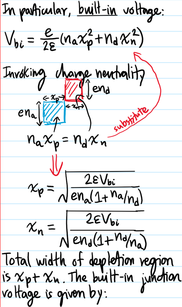
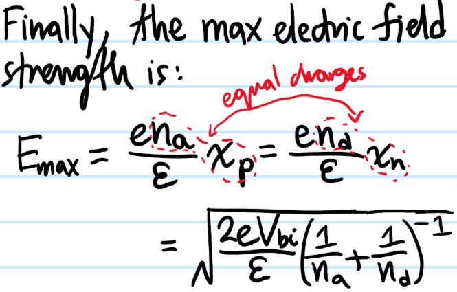
Problem: Make the sketches more quantitative. In particular, calculate the width \(x_n+x_p\) of the depletion region and the maximum strength \(E_{\text{max}}\) of the electrostatic field at the junction \(x=0\).
Solution:
Problem: Explain qualitatively how a depletion region forms at a \(p\)-\(n\) junction.
Solution: Intuitively, the electrons and holes cannot just keep diffusing indefinitely across the \(p\)-\(n\) junction because at some point too much like charge will clump on either side during recombination, preventing any further diffusion. Put another way, as the charge separation gets bigger and bigger, the induced \(\textbf E\)-field pointing from \(n\to p\) exerts an electric force on the electrons and holes that prevents them from crossing the junction; at equilibrium, this forms a depletion region where there are no mobile charge carriers.
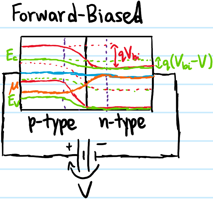
Problem: Just as a harmonic oscillator can be free or driven, so a \(p\)-\(n\) junction can also be “free” (just sitting there with its built-in potential \(V_{\text{bi}}\)) or it can be “driven” as well in a sense, more precisely by applying an external voltage \(V\) across it. However, unlike say with resistors/capacitors/inductors where the polarity of this voltage doesn’t really matter, here the asymmetry of the \(p\)-type vs. \(n\)-type semiconductors on either side, and thus the corresponding asymmetry of \(V_{\text{bi}}\), means that the polarity of \(V\) matters. Sketch qualitative band diagrams to show how the \(p\)-\(n\) junction’s bands change in the case of both forward bias \(V>0\) or reverse bias \(V<0\). This underlies the principle of operation for some (though not all) kinds of diodes, sometimes called a \(p\)-\(n\) semiconductor diode.
Solution: Some words of explanation: forward biasing a \(p\)-\(n\) junction lowers the effective built-in potential from \(V_{\text{bi}}\mapsto V_{\text{bi}}-V\). This clearly increases conductivity of both electrons and holes across the junction now that the energy barrier is reduced. By contrast, reverse biasing a \(p\)-\(n\) junction only raises the effective built-in potential \(V_{\text{bi}}\mapsto _{\text{bi}}+V\), reducing conductivity of electrons and holes as the depletion region gets bigger.
When the \(p\)-\(n\) junction is initially unbiased so that \(V=0\):
After forward biasing \(V>0\):
The reverse-biased case is just opposite to the forward-biased case, and not shown. Note also that this is not an instance of quantum tunnelling, because it’s not just a simple top-hat potential barrier, there is no probability current across the depletion region, and indeed also no electric current, only diffusion current as elaborated later.
Another way to put it is that forward-biasing the \(p\)-\(n\) junction encourages the majority charge carriers on each side to diffuse across the depletion region (and discourages the minority carriers, but that doesn’t matter anyways because they are minority), while reverse-bias is the opposite.
Problem: Recall that in an intrinsic semiconductor, at finite \(T>0\), the very few charge carriers in the conduction band are purely thermal electrons excited from their corresponding thermal holes in the valence band. Then, respectively \(p\)-type or \(n\)-type doping the intrinsic semiconductor, the creation of hydrogenic acceptor states just above the valence band or donor states just below the conduction band causes respectively holes to become the majority charge carrier (in the valence band) and electrons to become the minority charge carrier (in the conduction band) in the \(p\)-type extrinsic semiconductor, and vice versa for \(n\)-type (that isn’t to say that the thermal electrons and thermal holes \(n_{e^-,i}=n_{h^+,i}=n_i\sim 1.5\times 10^{10}\text{ cm}^{-3}\) aren’t still there, just they become negligible).
Solution:
Problem: Calculate the reverse saturation current \(I_{\text{sat}}=\lim_{V\to-\infty}I_{\text{sat}}(e^{V/V_T}-1)\) for a \(p\)-\(n\) junction semiconductor diode with the following parameters:
\[n_a=\]
To sort out later:
At T=0 K, mu is not really well-defined (b/c g(E)=0 in the band gap, so mu could be put anywhere in there..) but for T>0 K it is well-defined…
For n-type doping, by putting extra atoms near the bottom of the conduction band, will increase the chemical potential…(all this comes from interpreting mu as a silly fit parameter that needs to be tuned to get integral g(E)f(E) = number density of conduction electrons in the system = number density of donor dopants).
For p-type doping, add strongly electronegative atoms, they rip off electrons from the valence band. leaving additional holes in the valence band.
w.r.t. intrinsic concentrations of electrons and holes at T=300 K,
something about asymmetry of the densities of states…the presence of the donor and acceptor states in the band gap influences g(E) there…
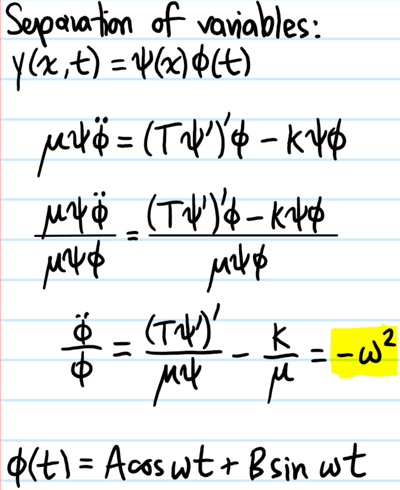
Problem: A vibrating string with displacement profile \(y(x,t)\) has non-uniform mass per unit length \(\mu(x)\) and non-uniform tension \(T(x)\) experiences both an internal restoring force due to \(T(x)\) but also a linear “Hooke’s law” restoring force \(-k(x)y(x)\) everywhere so that its equation of motion is governed by:
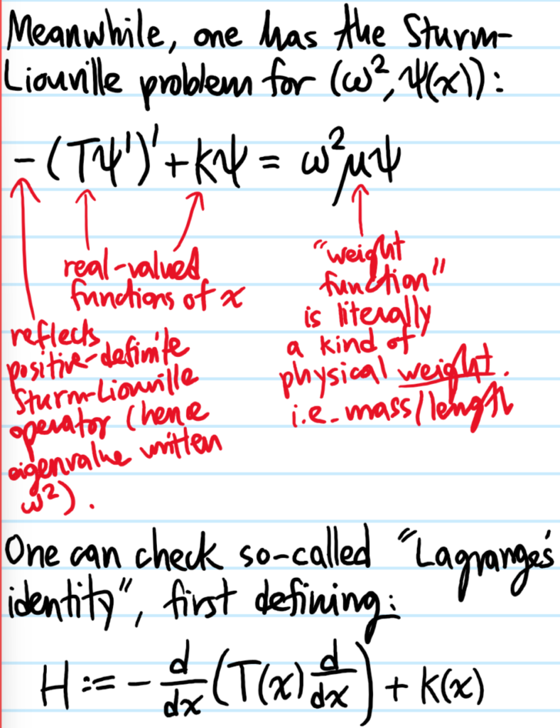
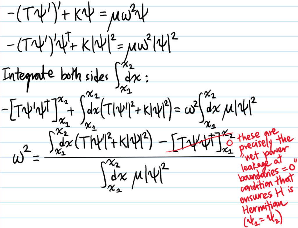
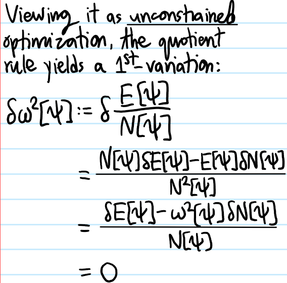
Problem: Make the “Noetherian interpretation” above more concrete by showing that the eigenvalue \(\omega^2\) can be expressed as a Rayleigh-Ritz quotient:
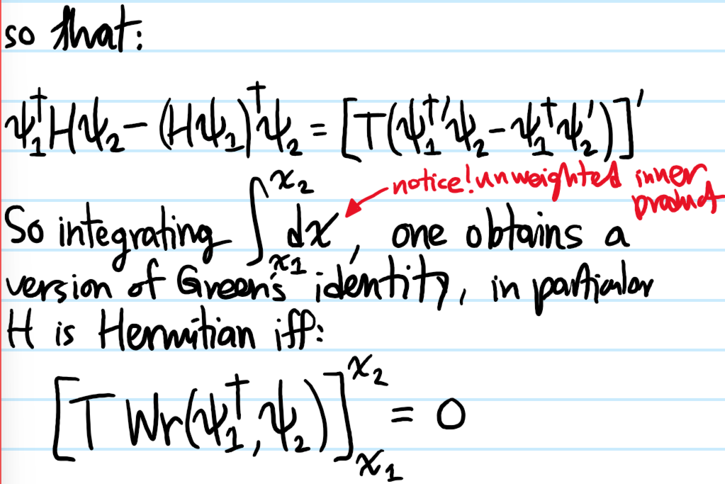
making it look like the usual Rayleigh-Ritz quotient employed in the quantum mechanical variational principle (although this glosses over the subtlety about boundary terms in the integration by parts).
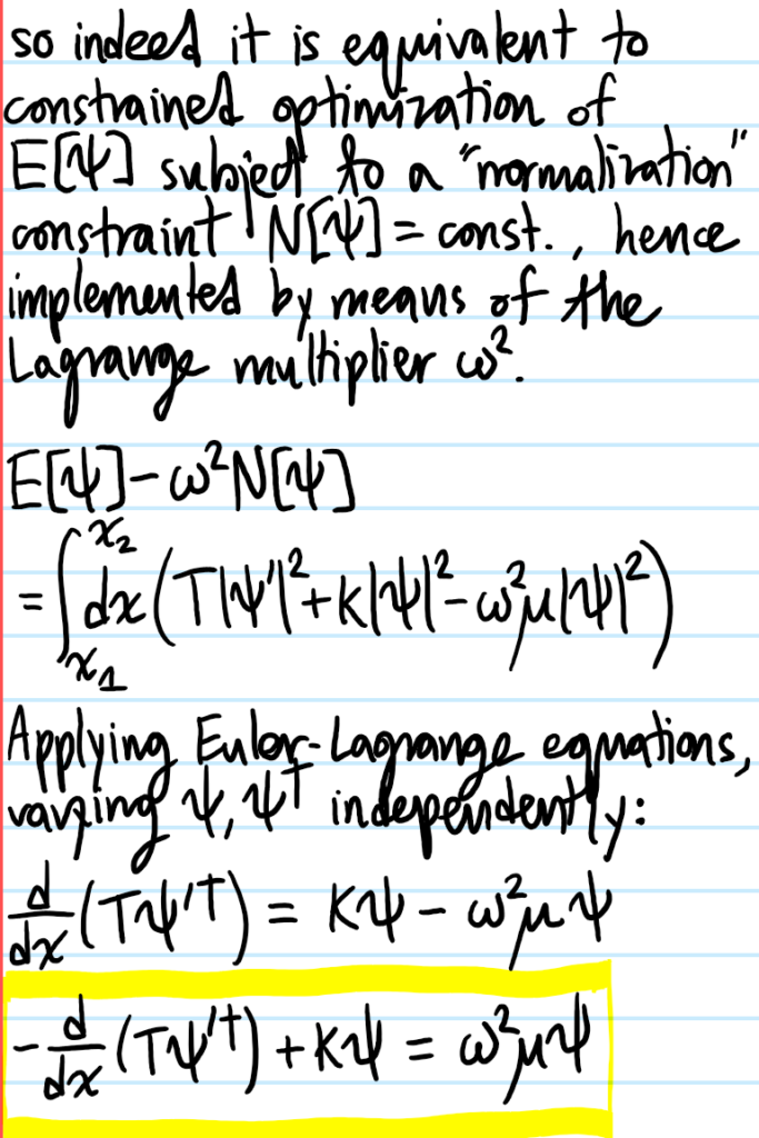
Problem: Conversely, show that if one considers \(\omega^2=\omega^2[\psi]\) as a functional of \(\psi(x)\), then the functional is stationary on eigenstates \(\psi\) of the Sturm-Liouville operator \(H\) and with eigenvalue \(\omega^2[\psi]\).
Solution:
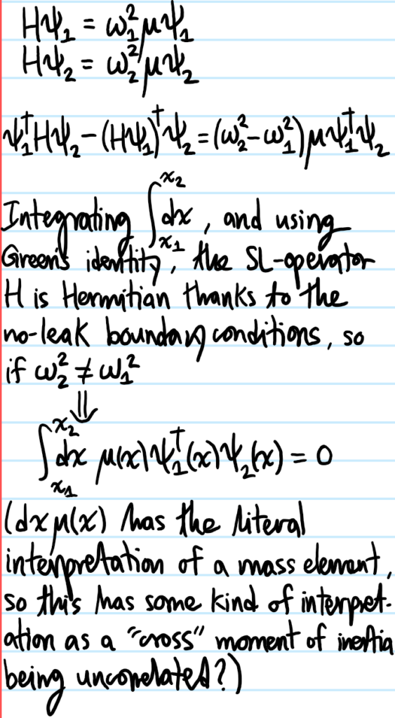
Problem: Show that eigenfunctions of the Sturm-Liouville operator with distinct eigenvalues are \(\mu\)-orthogonal.
Solution: (this proof assumes the eigenvalues have already been shown real, and the proof of that essentially mirrors this proof except setting \(1=2\)):
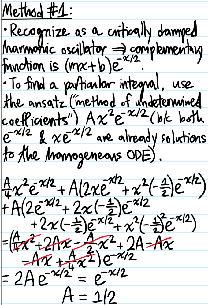
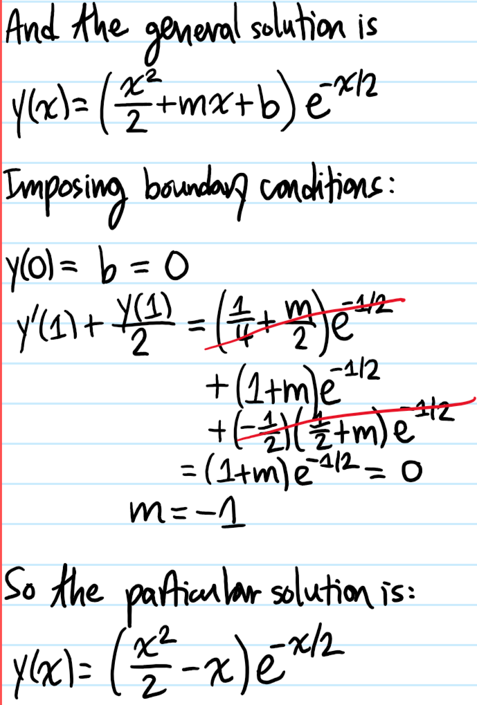
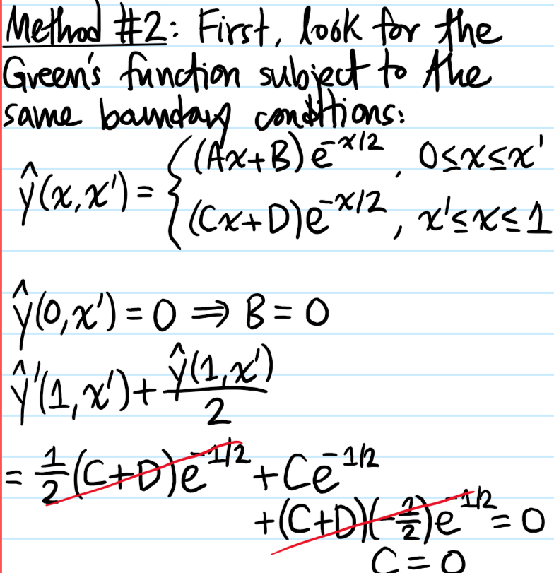
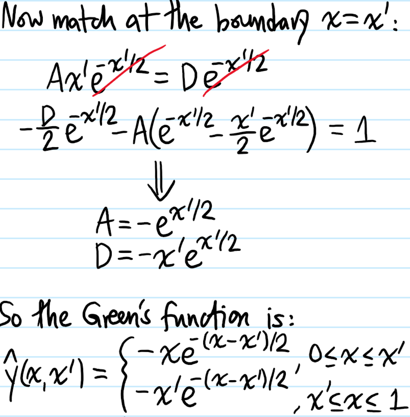
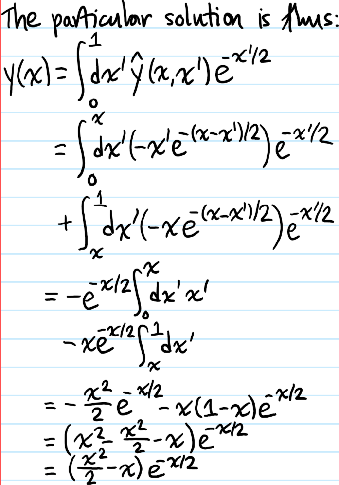
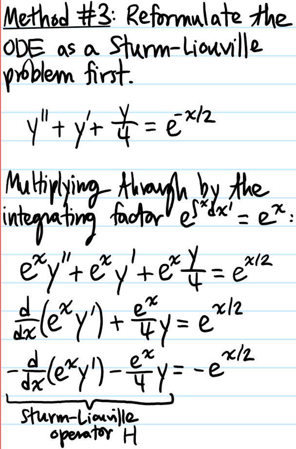
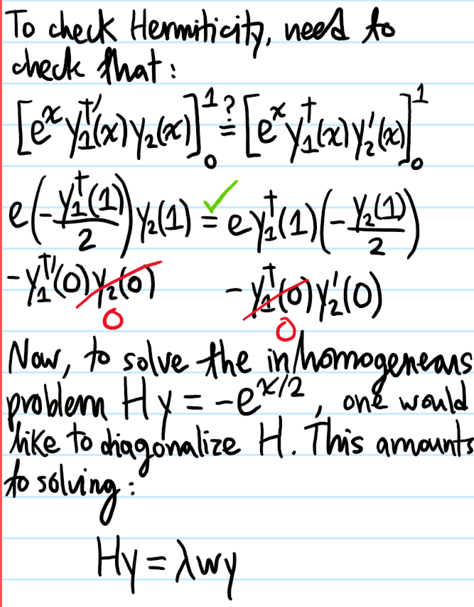
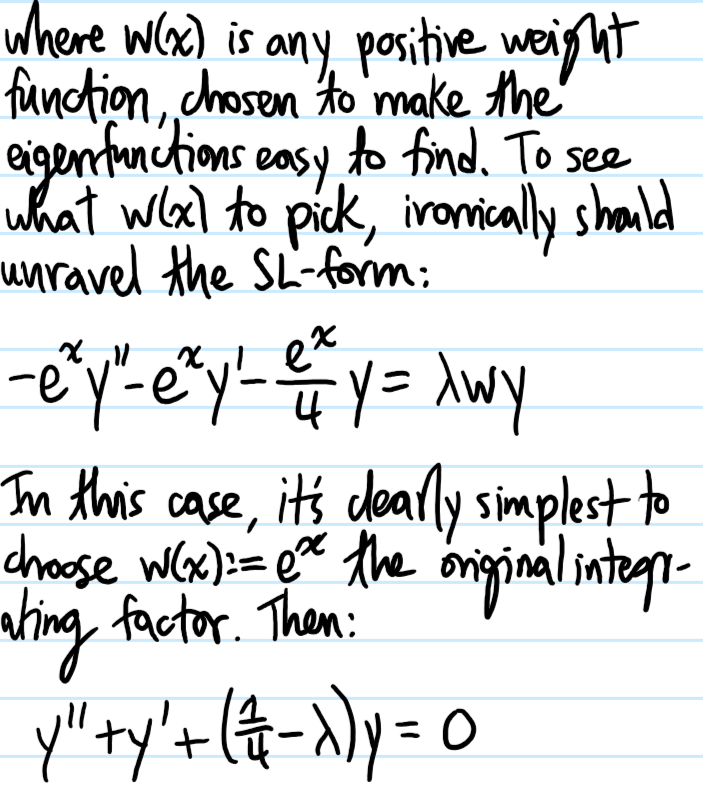
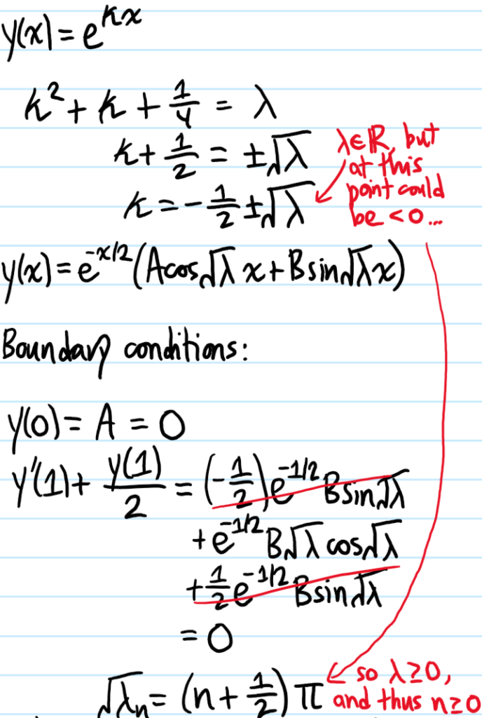
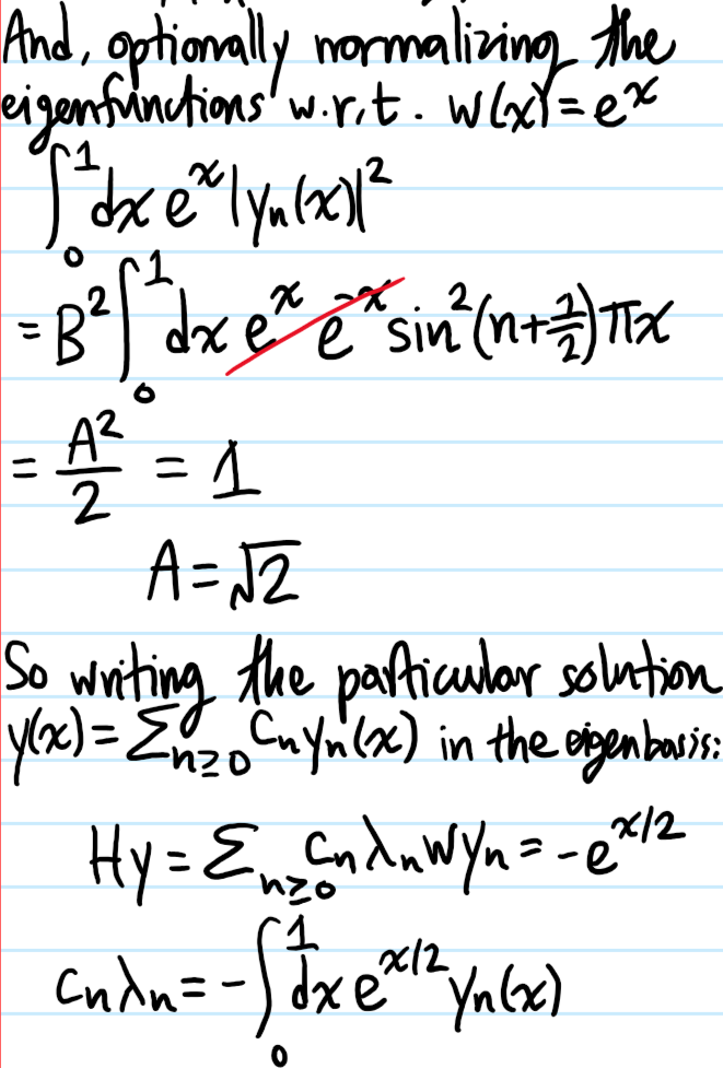
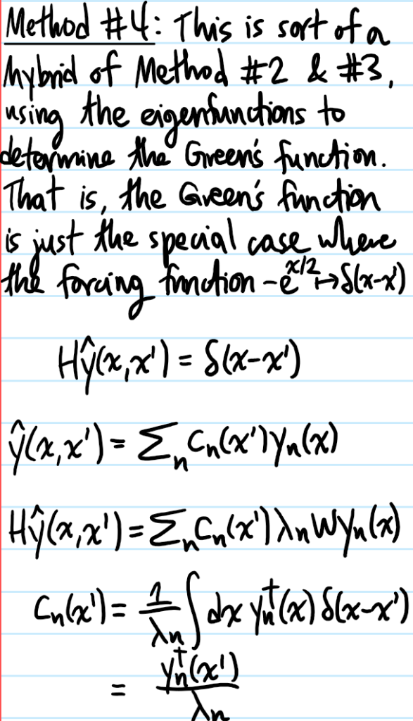
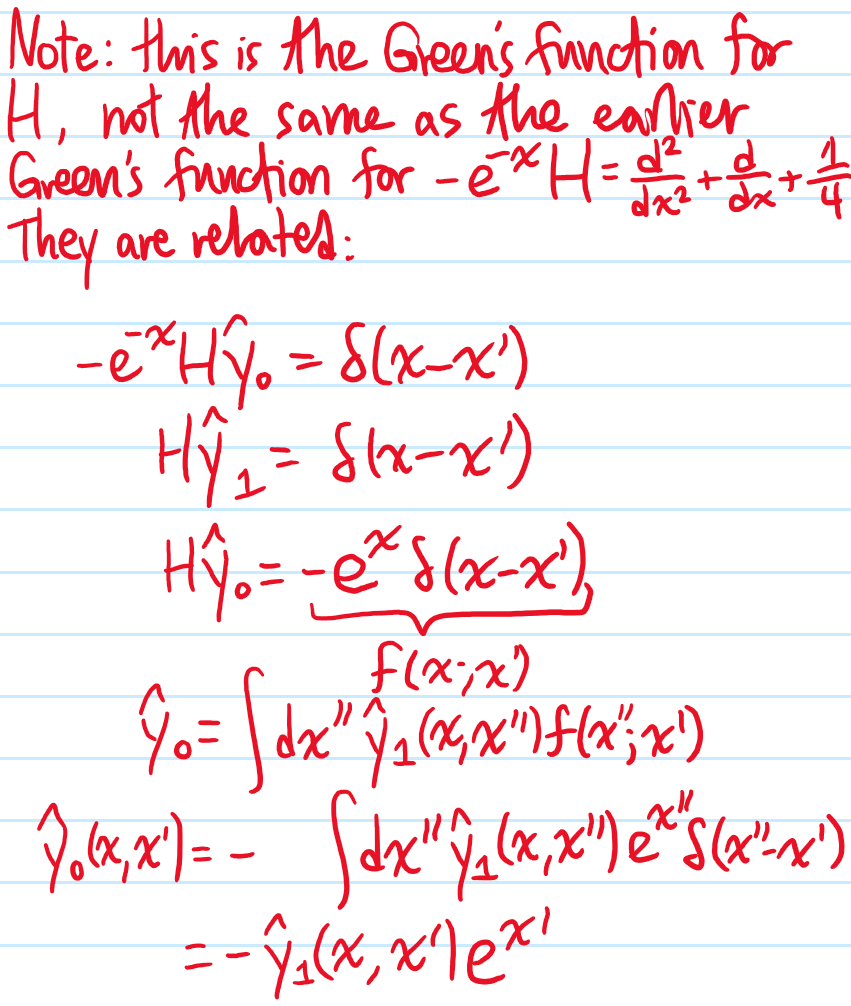
Problem: Solve the following inhomogeneous \(2^{\text{nd}}\)-order ODE:
Learning physics is hard. The purpose of this post is to collect a bunch of techniques that can help to make the process of learning (and remembering!) new concepts easier.
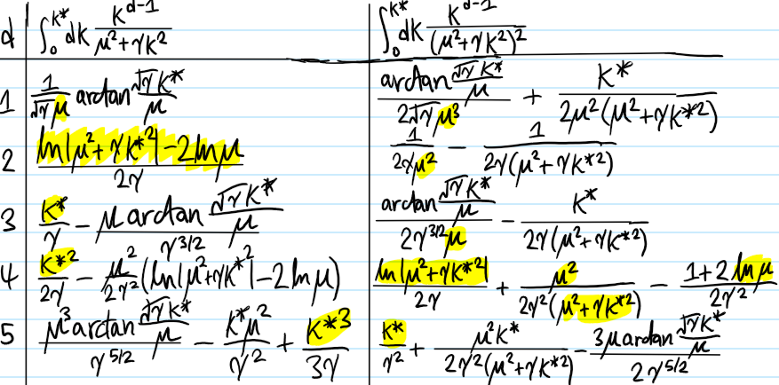
Tip #\(1\): Avoid always simplifying formulas as much as possible, group quantities in dimensionally useful combinations.
Explanation: Since elementary school, one is often taught to simplify everything as much as possible. While this is often a good idea if one is doing some calculation, sometimes a final result is better left unsimplified, especially if dimensionally intuitive quantities are grouped together.
Example: The density of states in \(k\)-space of an ideal electron gas, simplified, is:
\[g(k)=\]
However, it is much more preferable to remember it in the unsimplified form:
\[g(k)=\]
Example: The impedance \(Z\) of non-dispersive transverse displacement waves on a string of tension \(T\) and speed \(c\) is, when simplified, \(Z=\sqrt{Tc}\). However, it is preferable to remember it as:
\[Z=\frac{T}{\sqrt{T/c}}\]
since this reinforces that it’s just a “force/velocity”.
Tip #\(2\): Try covering up the microscopic inner workings with a black box.
Explanation: This is basically an engineering mindset. For instance, to use an op-amp, one does not have to understand the detailed transistor networks inside.
Example: A Fabry-Perot interferometer…looks like a diffraction grating viewed as a black box.
Tip #\(3\): Understand systems by isomorphism.
Explanation: Mathematicians love talking about (and finding) isomorphisms between various kinds of spaces and structures, since often one structure \(X\) and easier to understand than another structure \(Y\) but in fact both are really the same, so one can leverage one’s understanding of \(X\) in order to make sense of \(Y\).
Example: Electric circuits are not as intuitive to me as a damped, driven harmonic oscillator. Yet the \(2\) systems are in fact often isomorphic.
Tip #\(4\): Dimensional analysis! And don’t be afraid to package a lot of constants into one’s own custom-defined variables.
Explanation: As a general rule of thumb, use the least number of variable packages that eliminates all numerical factors (a catchy slogan to summarize this?).
Example: The dispersion relation for the \(n^{\text{th}}\) mode of waves propagating along the \(x\)-axis of a \(2\)D waveguide with fixed boundary conditions at \(y=0,\Delta y\) can be written:
This formula can be conceptually simplified by defining the cutoff frequency \(\omega_c:=\pi c/\Delta y\) so that:
\[\omega^2=c^2k_x^2+n\omega_c^2\]
Example: The dispersion relation for electromagnetic waves in a conductor at high frequencies can be written:
(plasma frequency)
Tip #\(5\): Build a “circuit model” of the system.
Explanation:
Example: A transmission line can be viewed as…
Tip #\(6\): Write formulas without any numerical prefactors, focusing on dimensional analysis.
Tip #\(7\): Remember some physical values of quantities in SI units, get a feel for orders of magnitude.
Example: Knowing that Avogadro’s constant is something like \(N_A\sim 10^23\) and Boltzmann’s constant is \(k_B\sim 10^{-23}\) (both when expressed in SI units), it follows that their product should be \(O(1)\) (again in SI units), and in this context one obvious \(O(1)\) constant is the gas constant \(R\approx 8.3\) so this helps to remember that:
\[N_Ak_B=R\]
Tip #\(8\): This tip applies specifically to studying new quantum systems. Basically, the algorithm for understanding is:
In other words, first have a clear idea of what the Hilbert state space \(\mathcal H\) of the system is, what the Hamiltonian \(H:\mathcal H\to\mathcal H\) is, and (the hard part that needs to be worked out carefully) the eigenstates \(|\psi\rangle\) and their corresponding eigenenergies \(E\). With that, essentially everything is thus known about the system such as its time evolution, the time evolution of expectation values of observables, and measurement probabilities.
Problem: What is an estimator \(\hat{\theta}\) for some parameter \(\theta\) of a random variable? Distinguish between point estimators and interval estimators.
Solution: In the broadest sense, an estimator is any function of \(N\) i.i.d. draws of the random variable \(\hat{\theta}(X_1,…,X_N)\). First, notice that the presence of the integer \(N\) is a smoking gun that all of the estimation theory that follows is strictly a frequentist approach rather than a Bayesian one.
Because \(X_1,…,X_N\) are random variables, it follows that \(\hat{\theta}\) is also a random variable. This definition doesn’t say anything about how good or bad the estimator \(\hat{\theta}\) needs to be with respect to actually trying to estimate the property \(\theta\) of the random variables.
Although the parameter \(\theta\) is fixed (in the frequentist interpretation), \(\hat{\theta}\) can either attempt to estimate \(\theta\) by directly giving a value (in which case \(\hat{\theta}\) is called a point estimator for \(\theta\)) or giving a range of values such that one has e.g. “\(95\%\) confidence” that \(\theta\) lies in that range (in which case \(\hat{\theta}\) is called an interval estimator for \(\theta\)).
Problem: Show that, if \(X_1,X_2,…,X_N\) are i.i.d. random variables, hence all having the same mean \(\mu=\langle X_1\rangle=…=\langle X_N\rangle\), then the random variable (called the sample mean):
\[\hat{\mu}:=\frac{X_1+X_2+…+X_N}{N}\]
is an unbiased point estimator for \(\mu\).
Solution: The purpose of this question is to emphasize what it means to be an unbiased point estimator, specifically one should compute the expectation:
so it is indeed unbiased or equivalently, there’s no systematic error \(\langle\hat{\mu}\rangle=\mu\).
Problem: Same setup as above, but now suppose one estimates the mean \(\mu\) using the estimator:
\[\hat{\mu}:=X_1\]
Explain why this is a bad choice of estimator.
Solution: First, notice that despite being “obviously bad”, this estimator is in fact unbiased \(\langle\hat{\mu}\rangle=\langle X_1\rangle=\mu\). However, as more and more instances of the random variable are instantiated \(N\to\infty\), this estimator \(\hat{\mu}\) remains the same forever (namely whatever the first draw happened to be). Thus, here the problem isn’t about bias, it’s about the inconsistency of the estimator (see: https://en.wikipedia.org/wiki/Consistent_estimator).
Problem: Show that, if \(X_1,X_2,…,X_N\) are i.i.d. random variables, hence all having the same mean \(\mu=\langle X_1\rangle=…=\langle X_N\rangle\) and same variance \(\sigma^2=\langle (X_1-\mu)^2\rangle=…=\langle (X_N-\mu)^2\rangle\), then the random variable (called the sample variance):
Solution: This is a very fun and instructive exercise. The key is to explicitly write out \(\hat{\mu}=\sum_{i=1}^NX_i/N\), use the parallel axis theorem \(\langle X^2_1\rangle=…=\langle X^2_N\rangle=\mu^2+\sigma^2\), and the independence assumption in i.i.d. so that in particular \(\langle X_iX_j\rangle=\mu^2+\delta_{ij}\sigma^2\).
Heuristically, this arises because \(\hat{\mu}\) has been estimated from the data \(X_1,…,X_N\) itself (as the proof above makes transparent) rather than an external source, thus representing a reduction in the number of degrees of freedom by \(1\), hence the so-called Bessel’s correction \(N\mapsto N-1\).
Problem: Even though \(\hat{\sigma}^2\) is an unbiased point estimator for the variance \(\sigma^2\), show that \(\sqrt{\hat{\sigma}^2}\) is a biased point estimator for the standard deviation \(\sigma\) (in fact, \(\sqrt{\hat{\sigma}^2}\) will systematically underestimate the actual standard deviation \(\sigma\)).
Solution: Because \(\langle\hat{\sigma}^2\rangle=\sigma^2\) is an unbiased point estimator of the variance, it follows that \(\sigma=\sqrt{\langle\hat{\sigma}^2\rangle}\). The result is thus obtained by an application of Jensen’s inequality to the concave square root function.
Problem: Show that the standard deviation of the the sample mean point estimator \(\hat{\mu}\) is given by (called the standard error on \(\hat{\mu}\)):
\[\sigma_{\hat{\mu}}=\frac{\sigma}{\sqrt{N}}\]
Solution: This follows from the usual result (Bienaymé’s identity) that the variance is a linear function of uncorrelated random variables, hence the standard deviation of \(\sum_{i=1}^NX_i\) is \(\sqrt{N}\sigma\), so because one then divides by \(N\) to obtain \(\hat{\mu}\), the result follows.
In practice of course, the standard deviation \(\sigma\) in that numerator of the standard error \(\sigma_{\hat{\mu}}\) isn’t known, and even worse the previous exercise just established that \(\langle\sqrt{\hat{\sigma}^2}\rangle\leq\sigma\) is a biased underestimate of the true standard deviation \(\sigma\). Nevertheless, if \(N\gg 1\), one expects \(\langle\sqrt{\hat{\sigma}^2}\rangle\to\sigma\) to be asymptotically unbiased, and hence the standard error estimator \(\hat{\sigma}_{\hat{\mu}}=\sqrt{\hat{\sigma}^2/N}\) is commonly used to estimate the true standard error \(\sigma_{\hat{\mu}}=\sigma/\sqrt{N}\) even if strictly a bit biased.
Problem: A poll is conducted to estimate the proportion of people in some country who support candidate \(A\) vs. candidate \(B\). A total of \(N=1000\) people are surveyed, and it is found that \(N_A=520\) support candidate \(A\). Report a \(95\%\) confidence interval for the actual proportion of people in the country who support candidate \(A\).
Solution: Each person can be taken as an i.i.d. \(p\)-Bernoulli random variable with value \(0\) if they support candidate \(B\) and \(1\) if they support candidate \(A\). Since \(\mu=p\) for a Bernoulli random variable, one has the unbiased point estimator:
\[\hat p=\frac{N_A}{N}=0.52\]
In order to report a \(95\%\) confidence interval, there are \(2\) additional assumptions that will be made. First, the central limit theorem asserts that \(p\) (a sum of \(N=1000\gg 1\) i.i.d. Bernoulli trials) will be approximately normally distributed with mean \(\hat{p}\) and standard error \(\sigma_{\hat p}=\sigma/\sqrt{N}=\sqrt{p(1-p)/N}\). Because \(p\) is unknown, the standard error can be estimated by \(\hat{\sigma}_{\hat p}=\sqrt{\hat p(1-\hat p)/N}\approx 0.016\), and from this one would report the confidence interval as:
with the \(z\)-score \(z\approx 1.96\) for the normal distribution (recalling the familiar \(68-95-99.7\) rule for normal distributions, it makes sense that \(z\approx 2\)).
Finally, a subtlety: this standard error estimator \(\hat{\sigma}_{\hat p}=\sqrt{\hat p(1-\hat p)/N}\) is actually not the same as the one mentioned earlier \(\hat{\sigma}_{\hat{\mu}}=\sqrt{\hat{\sigma}^2/N}\). One can explicitly check this and find that ultimately Bessel’s correction leads instead to the standard error estimator \(\hat{\sigma}_{\hat p}=\sqrt{\hat p(1-\hat p)/(N-1)}\) (in fact, in this case there’s also another subtlety: instead of using a \(z\)-score, one has to use a \(t\)-score associated to \(N-1=999\) degrees of freedom). For \(N\gg 1\), these \(2\) methods are essentially indistinguishable, so no need to lose sleep.
Problem: Above, the estimators were simply presented out of thin air, and properties such as their bias/variance/consistency were analyzed as an afterthought; however, show that they all arise within the single unifying framework of the maximum likelihood principle.
Solution: Having observed \(N\) i.i.d. draws \(\mathbf x_1,…,\mathbf x_N\) from some underlying random variable parameterized by \(\boldsymbol{\theta}\) (e.g. for a univariate normal random variable one could take \(\boldsymbol{\theta}=(\mu,\sigma^2)\)), the maximum likelihood estimator \(\hat{\boldsymbol{\theta}}_{\text{ML}}=\hat{\boldsymbol{\theta}}_{\text{ML}}(\mathbf x_1,…,\mathbf x_N)\) is given by maximizing the likelihood function of \(\boldsymbol{\theta}\):
Aside: at first glance, this seems a bit weird; any sane person’s first reaction would’ve been to instead maximize the reverse conditional probability!
where “MAP” stands for maximum a posteriori. This highlights very clearly the core difference between the frequentist school of thought (in which \(\boldsymbol{\theta}\) is simply treated as a fixed, background constant) and the Bayesian school of thought (in which there is a notion of \(\boldsymbol{\theta}\) being a random variable and hence it being well-defined to talk about its prior \(p(\boldsymbol{\theta})\)).
Back to the frequentist MLE approach, because \(\mathbf x_1,…,\mathbf x_N\) are i.i.d., one can factorize the joint probability as a product of marginals:
To avoid possible numerical underflow instabilities, one would like to convert this product into a sum. The usual way to do this is with a \(\log\) (arbitrary base). Since \(\log\) is moreover monotonically increasing, the MLE estimator is thus equivalent to maximizing the log-likelihood function:
But now notice that, instead of summing over all \(i=1,…,N\), one can instead sum over all distinct instantiations of the random variable, weighted by its empirical probability \(p_0(\mathbf x)\) based on the \(N\) training examples \(\mathbf x_1,…,\mathbf x_N\):
which, by instead considering the negative log-likelihood, can be reformulated as a problem of minimizing the cross-entropy \(S_{p(\boldsymbol{\theta})|p_0}\) of the model distribution \(p(\mathbf x|\boldsymbol{\theta})\) with respect to the empirical distribution \(p_0(\mathbf x)\):
For instance, success would mean finding a \(\boldsymbol{\theta}\) such that \(p(\boldsymbol{\theta})=p_0\) since in this case the KL-divergence \(D_{\text{KL}}(p(\boldsymbol{\theta})|p_0)=0\) attains its minimum possible value by virtue of the Gibbs inequality. Ideally, MLE would seek to choose \(\boldsymbol{\theta}\) so as to make \(p(\mathbf x|\boldsymbol{\theta})\) match the actual data-generating distribution \(p(\mathbf x)\), but since one doesn’t have access to this, the best one can hope for is to have \(p(\mathbf x|\boldsymbol{\theta})\) match the empirical distribution \(p_0(\mathbf x)\) as a proxy for the true \(p(\mathbf x)\).
Problem: In what sense can minimizing an MSE cost function of the parameters be justified from the perspective of maximum likelihood estimation?
Solution: The key assumption is that the possible target labels \(y\) associated to a given feature vector \(\mathbf x\) are normally distributed around some \(\mathbf x\)-dependent mean \(\hat y(\mathbf x|\boldsymbol{\theta})\) with some \(\mathbf x\)-independent variance \(\sigma^2\), i.e. \(p(y|\mathbf x,\boldsymbol{\theta})=(2\pi\sigma^2)^{-1/2}\exp -\frac{(y-\hat y(\mathbf x|\boldsymbol{\theta}))^2}{2\sigma^2} \). In practice, it’s hard to know this in advance; only after fitting \(\hat y(\mathbf x|\boldsymbol{\theta}_{\text{ML}})\) and plotting a histogram of the residuals \(\hat y(\mathbf x_i|\boldsymbol{\theta}_{\text{ML}})-y_i\) can one check a posteriori if the histogram looks Gaussian or not.
With this, the conditional log-likelihood \(-N\ln\sigma-\frac{N}{2}\ln(2\pi)-\frac{1}{2\sigma^2}\sum_{i=1}^N(\hat y(\mathbf x_i|\boldsymbol{\theta})-y_i)^2\) is clearly maximized for the same \(\boldsymbol{\theta}\) as the mean square error:
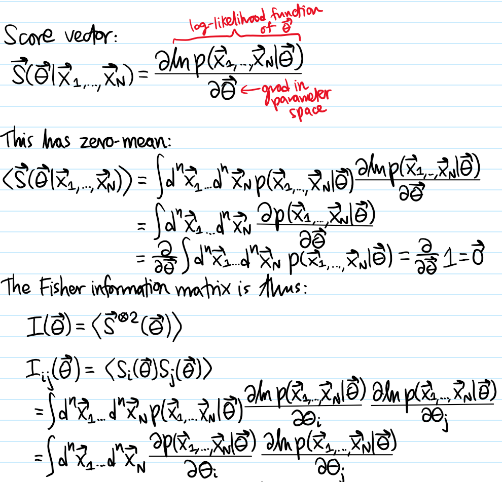
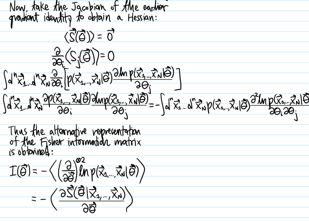
Problem: Define the score random vector \(\mathbf S(\boldsymbol{\theta})=\mathbf S(\boldsymbol{\theta}|\mathbf x_1,…,\mathbf x_N)\). Show that the covariance matrix of the score \(\mathbf S(\boldsymbol{\theta})\), called the Fisher informationmatrix \(I(\boldsymbol{\theta}):=\langle(\mathbf S(\boldsymbol{\theta})-\langle\mathbf S(\boldsymbol{\theta})\rangle)^{\otimes 2}\rangle\), may be written:
(all expectations \(\langle\space\rangle\) are of course over the joint distribution of the observed data \(\mathbf x_1,…,\mathbf x_N\) defined by the likelihood function \(p(\mathbf x_1,…,\mathbf x_N|\boldsymbol{\theta})\))
Solution:
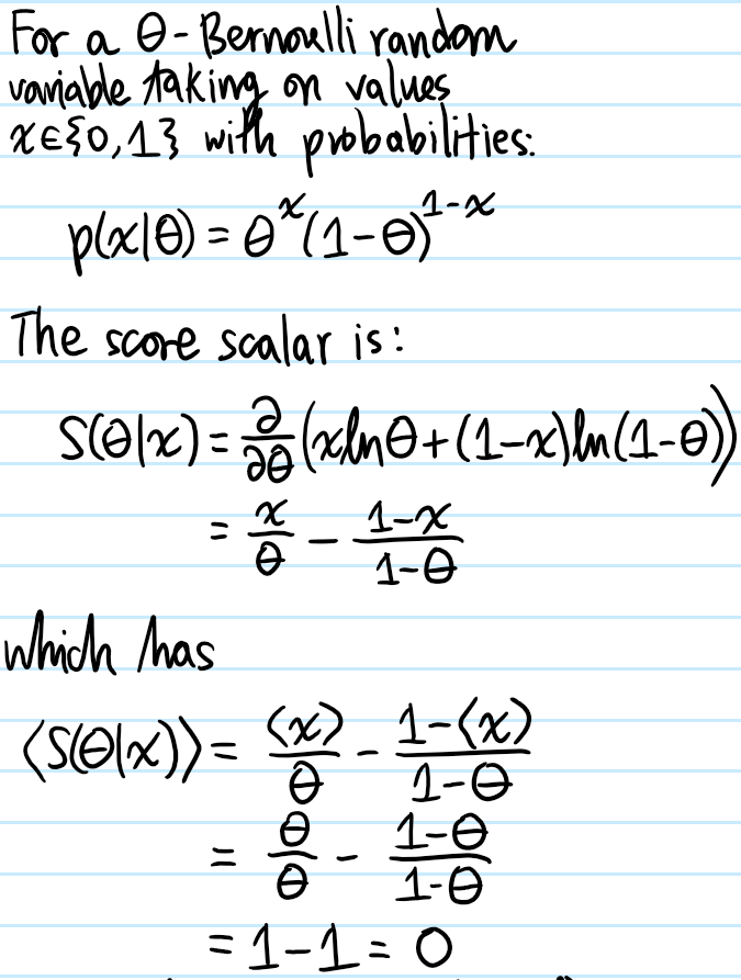
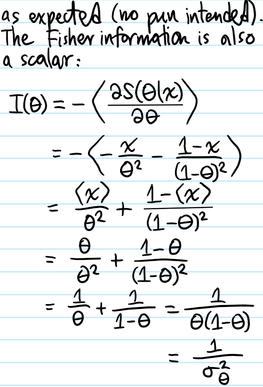
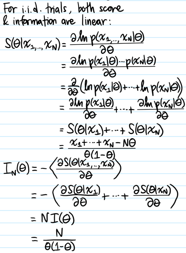
Problem: Calculate explicitly the score \(S(\theta|x)\) and Fisher information \(I(\theta)\) for a \(\theta\)-Bernoulli random variable with outcome \(x\in\{0,1\}\). Hence, what can be said about the score \(S(\theta|x_1,…,x_N)\) and Fisher information \(I_N(\theta)\) for the corresponding \(N\)-trial binomial random variable where each i.i.d. trial is \(\theta\)-Bernoulli?
Solution:
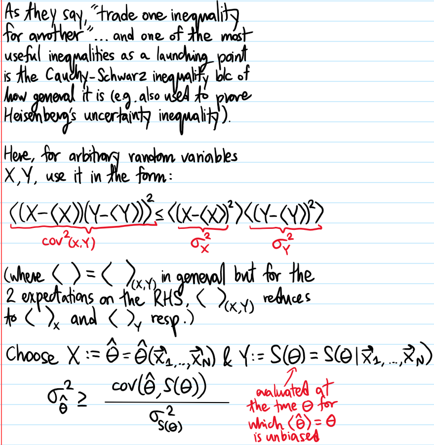
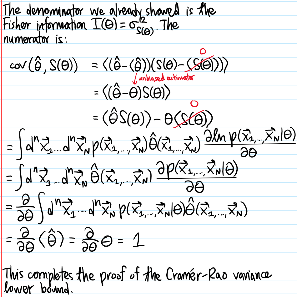
Problem: State and prove the Cramér-Rao variance lower bound.
Solution: Consider for simplicity attempting to estimate just a single, unknown, fixed scalar parameter \(\theta\) with an unbiased point estimator \(\hat{\theta}=\hat{\theta}(\mathbf x_1,…,\mathbf x_N)\). Then the Cramér-Rao variance lower bound asserts that the minimum possible variance of such an estimator \(\hat{\theta}\) is given by the inverse Fisher information evaluated at the true underlying value of the parameter \(\theta\) for which the point estimator \(\langle\hat{\theta}\rangle=\theta\) is unbiased:
In the more general case where \(\langle\hat{\boldsymbol{\theta}}\rangle=\boldsymbol{\theta}\) is an unbiased point estimator for more than \(1\) parameter, a natural generalization holds:
where \(I^{-1}(\boldsymbol{\theta})\) is the inverse of the Fisher information matrix, and the meaning of this matrix inequality is that \(\text{cov}(\boldsymbol{\theta},\boldsymbol{\theta})-I^{-1}(\boldsymbol{\theta})\) is positive semi-definite.
Problem: Combining the results of the previous \(2\) problems, what can be deduced?
Solution: Naturally, one is interested in finding the minimum-variance unbiased estimator(MVUE) for some parameter. But the Cramér-Rao variance lower bound is precisely a statement about how low the variance can go. In particular, for the \((N,\theta)\)-binomial random variable, since \(\hat{\theta}=\sum_{i=1}^Nx_i/N\) was already shown to be an unbiased estimator for \(\theta\), and moreover its variance \(\sigma^2_{\hat{\theta}}=\theta(1-\theta)/N=1/I_N(\theta)\) saturates the Cramér-Rao variance lower bound, it must therefore be the MVUE for \(\theta\)!
Problem: How can random error be reduced in a scientific experiment? What about systematic error?
Solution: The standard error \(\sigma_{\hat{\mu}}=\sigma/\sqrt{N}\) can be taken as a quantitative proxy for the effective random error from \(N\) i.i.d. measurements. This reveals that there are \(2\) ways to reduce the effective random error:
Reduce \(\sigma\) (e.g. cooling down electronics to mitigate Johnson noise).
Increase \(N\) (make more measurements).
Reducing systematic error is a completely different beast, and requires techniques such as calibration against a “gold standard”, differential measurements, etc.
Problem: Explain how the \(\chi^2\) goodness-of-fit test arises from maximizing a log-likelihood function subject to normally distributed errors between the data and the model.
Solution: The \(\chi^2\) statistic is basically just a rearrangement of the usual formula for variance to isolate for \(N=\chi^2\). Indeed, comparing \(\chi^2\ll N,\chi^2\approx N,\chi^2\gg N\) basically is the whole point of the test. The subtraction of the number of constraints from \(N\) is also reminiscent of the Bessel correction, and in fact the \(2\) are there for conceptually the same reason.
Just as the fundamental theorem of single-variable calculus \(\int_{x_1}^{x_2}f'(x)dx=f(x_2)-f(x_1)\) is the key insight on which the entire subject of single-variable calculus rests, there is an analogous sense in which one can consider a fundamental theorem of classical computing to be the key insight on which the entire field of classical computing rests. This is:
Fundamental Theorem of Classical Computing: The vector space \(\textbf N\) over the binary Galois field \(\textbf Z/2\textbf Z\) admits the countably infinite basis \(\textbf N=\text{span}_{\textbf Z/2\textbf Z}\{2^n:n\textbf N\}\) so that \(\text{dim}_{_{\textbf Z/2\textbf Z}}(\textbf N)=\aleph_0\). Put differently, the binary representation map \(n\in\textbf N\mapsto [n]^{(1,2,4,8,…)}\in \) is
From a physics perspective, one can loosely think of \(\textbf N\cong(\textbf Z/2\textbf Z)^{\oplus\infty}\) as the direct sum of infinitely many copies of the binary “vector space” \(\textbf Z/2\textbf Z\). By contrast, in the field of quantum computing, one instead has a vector space of the form \((\textbf C^2)^{\otimes N}\) for \(N\) qubits…and the multiplicative structure of the tensor product is much richer than the additive structure of the direct sum, hence the interest in quantum computing.
Knowing all this, it follows that any data \(X\) (e.g. an image file, an audio file, etc.) which can simply be “reduced to numbers” by some injection \(f:X\to\textbf N\) is also in principle just reduced to some bit string\((b_k)_{k=0}^\infty\) simply by taking each \(f(x)\in\textbf N\) for \(x\in X\) and writing out the binary representation of \(f(x)\). For instance, when \(X=\{a,b,c,…,x,y,z\}\) is the alphabet, then one possible injection (or encoding) is called the American Standard Code for Information Interchange\(\text{ASCII}:\{a,b,c,…,x,y,z\}\to\textbf N\) which maps for instance \(\text{ASCII}(a):=97\), \(\text{ASCII}(b):=98\), and so forth (strictly speaking, ASCII uses \(7\) bits to represent \(2^7=128\) characters of which \(26\) are the usual English alphabet letters in lower case while another \(26\) are uppercase English letters. There was even an extended ASCII which used \(8\) bits to represent \(2^8=256\) characters, but ultimately that was clearly insufficient for things like the Chinese language and so nowadays Unicode (with UTF-8 encoding, which stands for Unicode Transformation Format – 8 bit, or UTF-16, UTF-32, etc.) tends to be used in lieu of ASCII).
When storing numbers in memory (e.g. RAM, HDD, SSD) a computer can experience overflowerror (most computers have \(64\)-bit architecture, so can safely store up to \(2^{64}-1\)), roundofferror (this is especially relevant to floating point arithmetic), and precision errors.
An analog-to-digital converter (ADC) is just an abstraction for any function that maps an analog signal \(V(t)\), \(I(x,y)\), etc. to a digital signal \(\bar V_i,\bar I_{ij}\), etc. More precisely, one can consider an ADC to be a pair \(\text{ADC}=(f_s,\rho)\) where \(f_s\) is the sampling rate of the ADC in samples/second and \(\rho\) is the bit depth/resolution/precision at which the ADC quantizes data in bits/sample, thus the bit rate \(\dot b\) of the ADC is \(\dot b=f_s\rho\) and this is in general distinct from the baud rate \(\dot{Bd}\) of serial communication with the ADC by a factor \(\lambda:=\frac{\dot b}{\dot{Bd}}\geq 1\) which describes the number of bits per baud (see this Stack Overflow Q&A for an idea of the distinction).
For \(V(t)\) an analog signal in the time domain which is bandlimited by some bandwidth \(\Delta f\), the Nyquist-Shannon sampling theorem asserts that in order to avoid aliasing distortions when sampling \(V(t)\), one has to use \(f_s>\Delta f\). Equivalently, if \(f^*=\Delta f/2\) is the largest frequency present in \(V(t)\), then the sampling frequency needs to obey \(f_s>2f^*\). For instance, humans can hear audio up to \(f^*=20\text{ kHz}\), so audio ADCs (a fancy way of saying microphones) sample at \(f_s=48\text{ kHz}\). Cameras are just image ADCs, where now “samples” is replaced by “pixels” and so \(f_s\) might be better called “pixel frequency” (with units of pixels/meter rather than samples/second?) and the use of the RGB color space is fundamentally based on the biology of the human eye and its \(3\) types of cone cells, and conventionally each R, G, B channel has \(256\) levels (or \(1\) byte) of intensity quantization simply because that was empirically found to be sufficient (so the total bit depth of an RGB image is \(\rho=3\) bytes/pixel or \(24\) bits/px.
In practice, such data would likely be further compressed (either via lossless or lossy data compression algorithms). For instance, JPEG (lossy), PNG (lossless), run-length encoding (lossless), etc. for digital/bitmap/raster images, Lempel-Ziv-Welch (LZW) (lossless) compression, Huffman encoding (lossless), byte pair encoding, for text files, and perceptual audio encoding (lossy) which exploits the psychoacoustic quirks of the human auditory system such as auditory maskingand high frequency limits.
Computers& Logic Circuits
One abstract paradigm for understanding how a computer works is: input\(\to\)storage + processing\(\to\)output. Input is typically taken from sensors (e.g. keyboards, mouses, touchscreens, microphones, cameras), memory is handled by RAM, storage is handled by HDD/SSD, processing is done by the central processing unit(CPU) (an integrated circuit (IC)) where CPU = control unit + arithmetic logic unit (ALU) (both storage and processing use logic circuits made of many logic gates combined together), and output is a monitor, a speaker, an electric motor, an LED etc. Processing + memory are heavily interdependent, connected by a memory bus.
This excellent YouTube demonstration of implementing standard logic gates (e.g. buffers, NOT gates, AND gates, OR gates, XOR gates, NAND gates, NOR gates, etc.) using standard hardware on a solderless breadboard, notably transistors. So really, when it comes to processing data, a “computer” is an abstraction over “logic circuits” which itself is an abstraction over “logic gates” which itself is an abstraction over “bits” which itself is an abstraction over transistors and physical hardware that one actually touch and feel in the real world.
Our current computer (Microsoft Surface Studio \(2\)) has \(\sigma_{\text{RAM}}=32\text{ GB}\) and \(\sigma_{\text{SSD or C-Drive}}=1\text{ TB}\) (with Microsoft OneDrive providing an additional \(\sigma_{\text{OneDrive}}=1\text{ TB}\) of storage space).
The Internet
A computer network is topologically any strongly connected undirected graph where nodes represent computing devices (e.g. computers, phones, etc.) and edges are communicationchannels between a pair of computers. Common network topologies include the ring, star, mesh, bus, and tree topologies. Examples of computer networks include local area networks (LAN), wide area networks (WAN), data center networks (DCN), etc. with the Internet being a distributed packet-switched WAN. When designing the architecture of a computer network, one is interested in minimizing the distance (with respect to a suitable metric) that any piece of data \(D\) must travel to get from one computer to another.
At the level of physical hardware, data can be communicated between computers via copper category 5 (CAT5) twisted pair cables adhering to Ethernet standards. Fiber optic cables can also be used with Ethernet standards. Wi-Fi or Bluetooth communicates data via radio waves which suffer attenuation. Regardless, for all \(3\) of these line coding schemes (maps from abstract bits to a digital signal in the real world) we need to thank James Clerk Maxwell.
The informal notion of the “speed” of an internet connection (i.e. one of the communication channels mentioned earlier) between two computing devices \(X, Y\) is made precise by the bit rate \(\dot b_{(X,Y)}\) between the computing devices \(X\) and \(Y\). The bandwidth of that communication channel is then just the maximum bit rate \(\dot b^*_{(X,Y)}\) between \(X\) and \(Y\) (not to be confused with the signal processing notion of the bandwidth \(\Delta f\) of an analog signal). Another important factor is the latency \(\Delta t_{(X,Y)}\) of a given communication channel (i.e. just the delay). Running an Internet speed test for my computer with the measurement lab (M-lab) yields \(\dot b^{\text{downloads}}_{\text{(computer,M-lab)}}=650.7\frac{\text{Mb}}{\text s}\) and \(\dot b^{\text{uploads}}_{\text{(computer,M-lab)}}=732.0\frac{\text{Mb}}{\text s}\) and a latency of \(\Delta t_{\text{(computer,M-lab)}}=4\text{ ms}\)
Just like every house \(H\) has a physical address \(A_H\), in the WAN that we call the Internet, every computing device \(X\) has an Internet Protocol (IP) address \(\text{IP}_X\). When a computing device \(X\) transmits data packets \(D\) across a communication channel to another computing device \(Y\), \(X\) must specify the IP address \(\text{IP}_Y\) of \(Y\) in addition to providing its own IP address \(\text{IP}_X\) so that \(Y\) can reply to it. There are actually \(2\) common IP address protocols, IPv4 (a string of \(4\) bytes, leading to \(2^{32}\) possible IPv4 addresses) and IPv6 (a string of \(8\) hexadecimal numbers each up to \(0xFFFF\) for a total of \(2^{128}\) possible IPv6 addresses). IP addresses of computing devices may also be dynamic meaning that one’s Internet service provider changes it over time \(t\). Or, if one connects to a disjoint Wi-Fi network, then this will usually also mean a different IP address as each Wi-Fi provider (internet service provider) has a range of IP addresses it is allowed to allocate. By contrast, computing devices acting as servers(e.g. Google’s computers) often have static IP addresses (e.g. \(\text{IPv4}_{\text{Google computers}}=74.125.20.113\)) to make it easier for client computing devices to communicate quickly with.
In terms of actually interpreting what the numbers in an IP address mean, it turns out that it doesn’t have to be the case that (say in an IPv4 address) each byte corresponds to some piece of information. Rather, one can decide how one wishes to impose a hierarchy of subnetworks (subnets) on the IP address, that is, how many bits to represent a given piece of information. This is sometimes known as “octet splitting” where “octet” = “byte” in an IPv4 address.
The Domain Name System (DNS) is essentially a map \(\text{DNS}:\{\text{URLs}\}\to\{\text{IP addresses}\}\) and indeed anytime one uses a browser application (e.g. Chrome) to search for a website URL (e.g. www.youtube.com), DNS servers need to first find the IP address \(\text{DNS}\)(www.youtube.com) associated with that URL.
Problem: Given a linear operator \(H\) on some vector space, define the resolvent operator \(G_H(E)\) associated to \(H\).
Solution: The resolvent \(G_H(E)\) of \(H\) is the operator-valued Mobius transformation of a complex variable \(E\in\textbf C\) defined by the inverse:
\[G_H(E):=\frac{1}{E1-H}\]
(this notation \(A/B\) is only unambiguous when \([A,B^{-1}]=0\) which it is in this case).
Problem: What is the domain for \(E\in\textbf C\) of the resolvent \(G_H(E)\)?
Solution: Any value of \(E\in\textbf C\) for which the matrix \(E1-H\) is invertible leads to a well-defined resolvent. But invertibility is equivalent to a non-vanishing determinant \(\det(E1-H)\neq 0\). However, when \(\det(E1-H)=0\), then \(E\) is an eigenvalue of \(H\). So the domain of \(G_H(E)\) is \(E\in\textbf C-\text{spec}(H)\).
Problem: To see the conclusion of Solution #\(2\) another way, assume \(H\) is Hermitian so that it admits a real orthonormal eigenbasis \(H|n\rangle=E_n|n\rangle\). Show that the resolvent \(G_H(E)\) of \(H\) may be expressed as a linear combination of projectors onto its eigenspaces:
where the matrix element is \(\langle n|\frac{1}{E1-H}|m\rangle=\frac{\delta_{nm}}{E-E_n}\). Thus, the resolvent has a simple pole whenever \(E=E_n\) for some \(H\)-eigenstate \(|n\rangle\), and its residue at that simple pole is given by the corresponding projector \(|n\rangle\langle n|\).
Problem: Define the retarded resolvent \(G_H^+(E)\) and the advanced resolvent \(G_H^-(E)\).
Solution: Killing \(2\) birds with \(1\) stone:
\[G_H^{\pm}(E):=G_H(E\pm i0^+)\]
so if \(H\) were Hermitian, then normally the poles of \(G_H(E)\) would all lie on the real axis; the retarded and advanced resolvents therefore exist to shift these poles slightly above or below the real axis.
Problem: Define the Fourier transform of the time evolution operator \(U_H(t)=e^{-iHt/\hbar}\) to a new operator-valued function of \(E\) given by the convention:
Show that \(U_H(E)=-\frac{1}{\pi}\Im G_H^+(E)=\frac{1}{\pi}\Im G_H^-(E)\), where the imaginary part of an operator is defined in the obvious manner.
Solution: One way is to proceed by direct evaluation, which gives \(U_H(E)=\delta(E1-H)\). On the other hand, any delta function can be written via a partial fraction expansion of a nascent delta given by eliminating the principal value of the Sokhotski-Plemelj theorem:
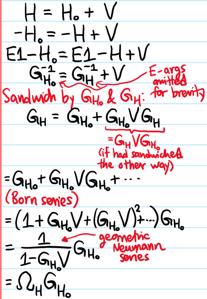
Problem:Starting from the decomposition \(H=H_0+V\), conclude that the resolvents \(G_H,G_{H_0}\) of \(H\) and \(H_0\) are related by:
\[G_H=\Omega_HG_{H_0}\]
where the Moller scattering operator \(\Omega_H\) of \(H\) depends on the choice of decomposition \(H=H_0+V\):
\[\Omega_H:=\frac{1}{1-G_{H_0}V}\]
Solution:
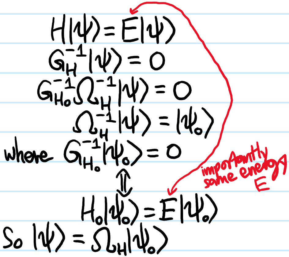
Problem: Starting from the Schrodinger equation \(H|\psi\rangle=E|\psi\rangle\) in the unusual form:
\[G^{-1}_H(E)|\psi\rangle=0\]
Use the result above to deduce the Lippman-Schwinger equation:
\[|\psi\rangle=\Omega_H|\psi_0\rangle\]
where \(H=H_0+V\) can be decomposed in any way one pleases, so long as this is reflected in the Moller scattering operator \(\Omega_H\) and the “free state” \(|\psi_0\rangle\) with commensurate energy \(H_0|\psi_0\rangle=E|\psi_0\rangle\) (thus, \(\Omega_H\) is “energy-conserving”).
Solution:
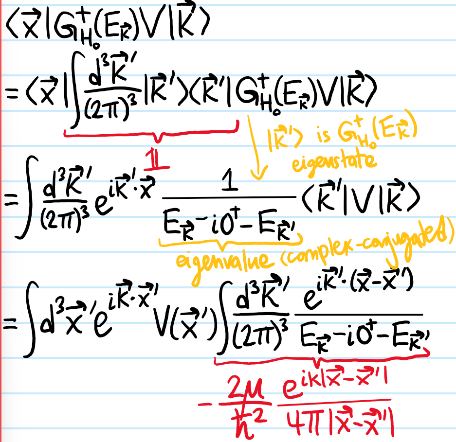
Problem: How is this form of the Lippman-Schwinger equation typically applied to quantum mechanical scattering?
Solution: The decomposition is chosen such that \(H_0=|\textbf P|^2/2\mu\) is a purely kinetic Hamiltonian and \(V\) is a corresponding \(2\)-body scattering potential for two particles of reduced mass \(\mu\) (working in the ZMF). In this case, one typically takes \(|\psi_0\rangle:=|\textbf k\rangle\) to be a plane wave \(H_0\)-eigenstate with energy \(E_{\textbf k}=\hbar^2|\textbf k|^2/2\mu\). Furthermore, one typically chooses the retarded Moller scattering operator \(\Omega_H^+(E_{\textbf k})=\frac{1}{1-G_{H_0}^+(E_{\textbf k})V}\) as an ad hoc way of cherrypicking the physical, outward-propagating solution \(|\psi\rangle:=|\psi^+_{\textbf k}\rangle\). Finally, it is convenient to work in a specific basis, typically the \(\textbf X\)-eigenbasis. Altogether then, the useful form of the Lippman-Schwinger equation for scattering theory is:
To actually evaluate this, one ultimately has to unwrap the earlier geometric Neumann series for \(\Omega^+_H(E_{\textbf k})=1+G^+_{H_0}(E_{\textbf k})V+…\) and perhaps truncate at some partial sum to yield a Born approximation to \(\psi_{\textbf k}^+(\textbf x)\):
Gauge-fixing the \(\textbf X\)-eigenstates to be an orthonormal basis in the sense that \(\langle\textbf x|\textbf x’\rangle=\delta^3(\textbf x-\textbf x’)\) and \(\int d^3\textbf x|\textbf x\rangle\langle\textbf x|=1\), and having implicitly assumed the normalization \(\langle\textbf x|\textbf k\rangle = e^{i\textbf k\cdot\textbf x}\), then one has \(\langle\textbf k|\textbf k’\rangle=(2\pi)^3\delta^3(\textbf k-\textbf k’)\) and \(\int\frac{d^3\textbf k}{(2\pi)^3}|\textbf k\rangle\langle\textbf k|=1\). Hence:
Problem: Is this perturbation theory?
Solution: It’s not really perturbation theory in the sense that the energies are just taken to be \(E=\hbar^2|\textbf k|^2/2m\), rather one is much more interested in the eigenstates (asymptotically especially!) from which other kinds of data like scattering amplitudes and cross sections, etc. are more interesting. So the goals of the \(2\) programs are different.
Problem: Consider some \(H_0\)-eigenstate \(|0\rangle\) with energy \(H_0|0\rangle=E_0|0\rangle\). Evaluate the expectation \(\langle 0|G_{H_0}(E)|0\rangle\). Hence, for \(H=H_0+V\), show that \(\langle 0|G_H(E)|0\rangle\) looks the same as \(\langle 0|G_{H_0}(E)|0\rangle\) except with \(E_0\mapsto E_0+\Sigma_H(E;|0\rangle)\) where the self-energy \(\Sigma_{|0\rangle,V}(E)\in\textbf C\) of the \(H_0\)-eigenstate \(|0\rangle\) due to the perturbation \(V\) is given by the usual:
where \(V_{nm}:=\langle n|V|m\rangle\) are the matrix elements of the perturbation \(V\) in the unperturbed \(H_0\)-eigenbasis.
Problem: What are the interpretations of \(\Re\Sigma_{|0\rangle,V}(E)\) and \(\Im\Sigma_{|0\rangle,V}(E)\)?
Solution:
By tracking the movement of a simple pole \(E_n\) of \(G_H(E)\) in the complex \(E\)-plane, one can recover the eigenvalue and eigenstate corrections of perturbation theory.
Solution: Shine the spotlight on some eigenstate \(|n\rangle\) and its associated energy \(E_n\) by separating the unperturbed resolvent as:
The first term in the sum turns \(E=E_n\) from a simple pole into a double pole. It turns out this is what’s responsible for shifting the location of the pole away from \(E=E_n\), in other words, perturbing the eigenvalue. Meanwhile the series in the middle contributes to the residue at \(E=E_n\) because \(m\neq n\). Clearly they must be responsible for perturbing the eigenstate. Finally, because \(m,\ell\neq n\) in the last sum, it will be analytic in a neighbourhood of \(E=E_n\), in other words: crap.
Strictly speaking, after including the \(G_{H_0}VG_{H_0}\) term from the geometric Neumann-Born-Laurent series, the pole still sits at \(E=E_n\), just that its order has increased from \(1\to 2\). But consider as an example the geometric series \(1+1/x+1/x^2+…\). For any finite partial sum truncation, the pole sits at \(x=0\). But for \(|x|>1\) this converges absolutely to \(x/(x-1)\) where now the pole has been displaced to \(x=1\). Or just take any function like \(\tan(x)\) and Taylor expand it around \(x=0\) say; although all the terms in that Taylor series are analytic, the limiting behavior must be non-analytic at \(x=\pm\pi/2\). It’s basically a more extreme version of a phase transition, since singularities are more extreme than discontinuities.
Anyways, the fact that its the expectation \(\langle n|V|n\rangle\) which is sitting in the numerator of the double pole term means that this is the \(1^{\text{st}}\)-order correction to the energy. Similarly, decomposing into partial fractions:
only the first term \(\sim(E-E_n)^{-1}\) contributes to the residue at \(E=E_n\), and moreover this eigenstate contribution is just \(\sum_{m\neq n}\frac{\langle m|V|n\rangle}{E_n-E_m}|m\rangle\). Continuing to higher-order terms in the expansion reproduces the next formulas.
Problem #\(6\): Let \(H=H(\lambda)\) be a non-degenerate Hamiltonian depending on a parameter \(\lambda\) (not necessarily infinitesimal), and let \(|n\rangle=|n(\lambda)\rangle\) be a normalized \(H\)-eigenstate with energy \(E_n=E_n(\lambda)\). By differentiating the spectral equation:
\[H|n\rangle=E_n|n\rangle\]
with respect to \(\lambda\), prove the Hellman-Feynman theorems for the rate of change of the eigenvalue \(E_n\) and the \(H\)-eigenstate \(|n\rangle\):
This is like having \(2\) vectors \((a,b,c)=(d,e,f)\); naturally one’s instinct would be to equate components \(a=d,b=e,c=f\). In this context, what that looks like is projecting both sides onto an arbitrary \(H\)-eigenstate \(|m\rangle\) to equate the scalar components of all vectors:
the Hellman-Feynman theorems then arise by considering the \(2\) cases \(m=n\) and \(m\neq n\). There is a priori also a component of the rate of change \(\partial|n\rangle/\partial\lambda\) of the \(H\)-eigenstate \(|n\rangle\) along itself with amplitude \(\langle n|\frac{\partial|n\rangle}{\partial\lambda}\), but due to normalization \(\langle n|n\rangle=1\Rightarrow\frac{\partial\langle n|}{\partial\lambda}|n\rangle+\langle n|\frac{\partial|n\rangle}{\partial\lambda}=0\Rightarrow\Re\langle n|\frac{\partial|n\rangle}{\partial\lambda}=0\Rightarrow\langle n|\frac{\partial|n\rangle}{\partial\lambda}=0\); this is like saying that an ant crawling on a sphere \(|\textbf x|^2=\text{const}\) must have orthogonal position and velocity \(\textbf x\cdot\dot{\textbf x}=0\).
The Hellman-Feynman theorems are reminiscent of formulas such as:
in which one takes \(A=H\) and \(\lambda=t\), as well as the special case \(\phi=\psi\) of Ehrenfest’s theorem.
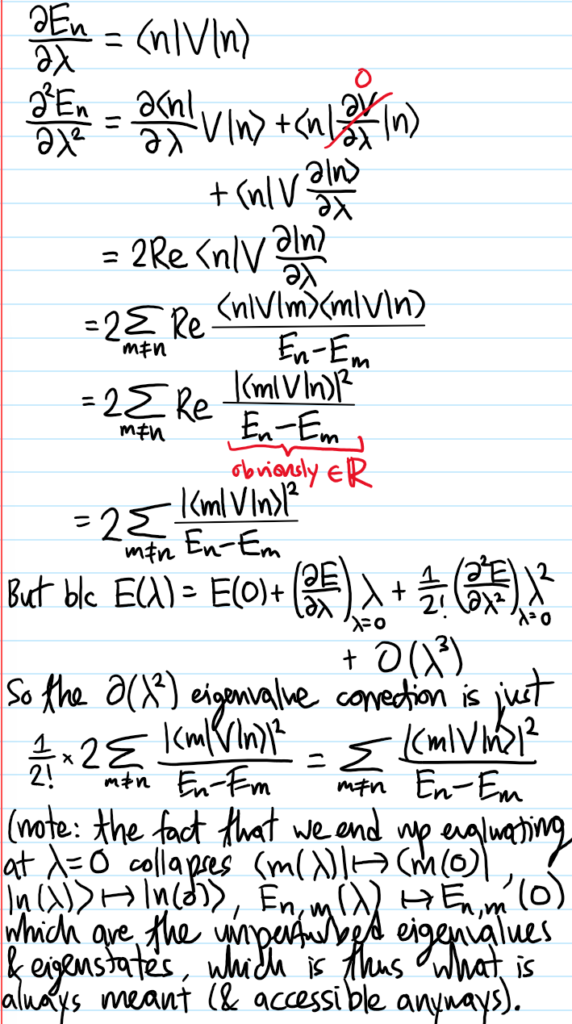
Problem #\(7\): Hence, by applying the Hellman-Feynman theorems to a linearly perturbed Hamiltonian \(H=H_0+\lambda V\), deduce the \(O(\lambda^2)\) corrections to both the eigenvalues \(E_n\) and eigenstates \(|n\rangle\) of the unperturbed Hamiltonian \(H_0\) in the presence of a perturbation \(V\).
Solution #\(7\): Specialized to the case of this particular linearly perturbed Hamiltonian, one has trivially \(\frac{\partial H}{\partial\lambda}=V\). With this in mind, one simply takes the Hellman-Feynman formulas and differentiate them again with respect to \(\lambda\):
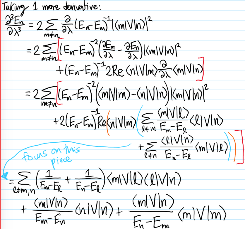
For fun, here is a (failed!) attempt to compute the \(O(\lambda^3)\) eigenvalue correction (what’s the mistake?):
And for the \(O(\lambda^2)\) eigenstate correction, refer to this document.
TO DO: extend/generalize all the above discussion to degenerate and time dependent perturbation theory! Also find where to put the following snippets:
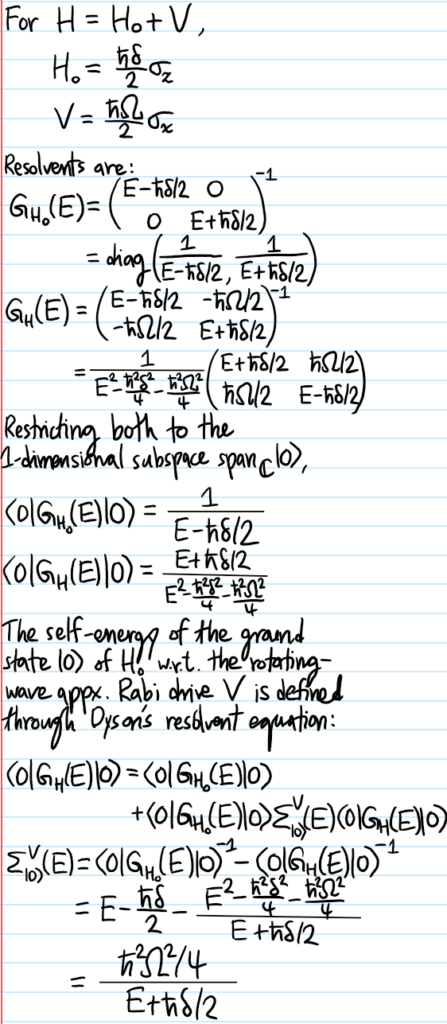
Problem: In the rotating frame of a Rabi drive \((\omega,\Omega)\) detuned by a small amount \(\delta:=\omega-\omega_0\) from a bare resonance, within the rotating wave approximation one has \(H=H_0+V\) with \(H_0=\frac{\hbar\delta}{2}\sigma_z\) and \(V=\frac{\hbar\Omega}{2}\sigma_x\). Evaluate the self-energy \(\Sigma^V_{|0\rangle}(E)\) in the one-dimensional subspace spanned by the ground state \(|0\rangle\), and show that it reproduces the \(2^{nd}\)-order AC Stark shift when evaluated on-shell (i.e. for \(E=-\hbar\delta/2\)).
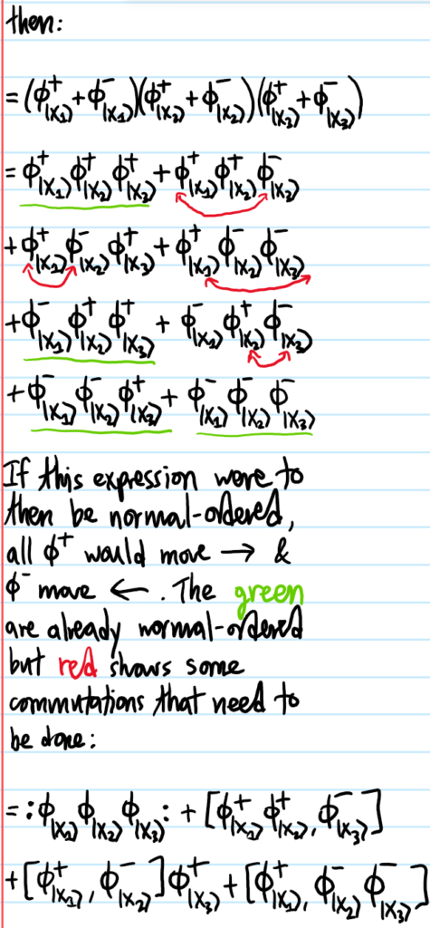
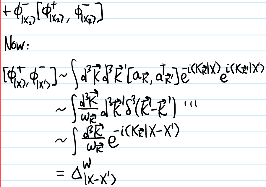
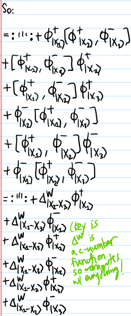
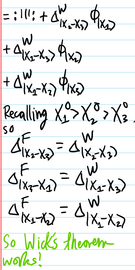
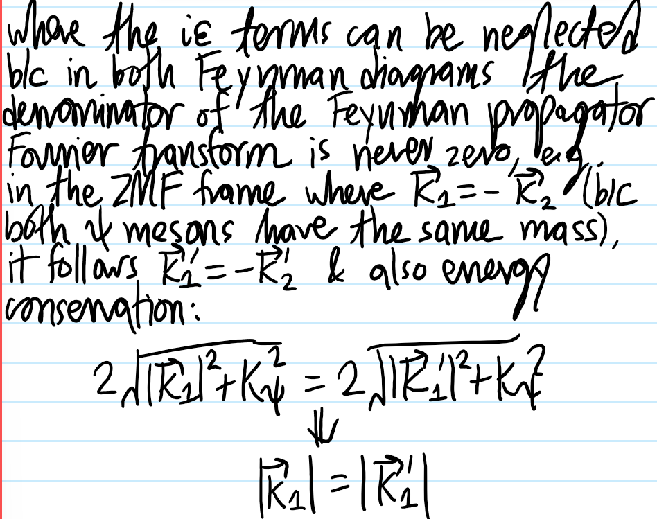
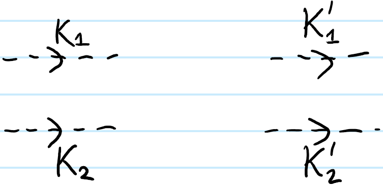
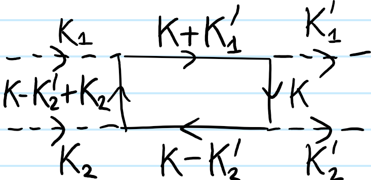
Although Feynman diagrams are often first encountered in statistical/quantum field theory contexts where they are employed in perturbative calculations of partition/correlation functions based on Wick’s theorem, there is a lot of “fluff” in these cases that obscures their underlying simplicity. The purpose of this post is therefore to build up to a simpler, intuitive view of what Feynman diagrams are really about that hopefully demystifies them.
of a univariate normally distributed random variable \(x\) with zero mean \(\langle x\rangle=0\) (the choice of zero mean is motivated by the fact that in practice one only cares about central moments of the distribution, so to avoid writing \(x-\langle x\rangle\) everywhere it is convenient to just set \(\langle x\rangle:=0\)).
Solution #\(1\): It is clear that for odd \(n=1,3,5,…\), the integrand is an odd function so not only is \(\langle x\rangle=0\) by construction, but all higher odd moments also vanish \(\langle x^3\rangle=\langle x^5\rangle=…=0\). As for even \(n=0,2,4,…\), there are several ways:
Way #\(1\): Start with the \(n=0\) normalization (obtained in the usual Poissonian manner):
and differentiate the equation by \(\frac{\partial}{\partial(-1/2\sigma^2)}\) to pull down arbitrarily many factors of \(x^2\). One finds for instance:
\[\langle x^2\rangle=\sigma^2\]
\[\langle x^4\rangle=3\sigma^4\]
\[\langle x^6\rangle=15\sigma^6\]
\[\langle x^8\rangle=105\sigma^8\]
and so forth, in general following the rule \(\langle x^{2m}\rangle=(2m-1)!!\sigma^{2m}\) for even \(n=2m\), where the double factorial can also be written in terms of single factorials as:
\[(2m-1)!!=\frac{(2m)!}{2^mm!}\]
Way #\(2\): Substitute for \(x^2/2\sigma^2\) to recast the integral in terms of a gamma function:
Problem #\(2\): From Solution #\(1\), the presence of factorials suggests a combinatorial interpretation of the result; what is this interpretation?
Solution #\(2\): Suppose one has \(6\) people that need to be paired up for a dance; how many pairings can be formed? There are \(2\) ways to think about this.
Way #\(1\): The first person can be paired with \(5\) other people. Then, after they’ve been paired, the next person can only pair up with \(3\) more people. And after they’ve paired, the next person can only pair with the \(1\) other person that’s left. So the answer is \(5!!=5\times 3\times 1=15\) pairs.
Way #\(2\): There are \(6!\) permutations of the \(6\) people. However, they are going to form \(3\) pairs which can be permuted in \(3!\) ways. And within each of the \(3\) pairs, there are a further \(2!=2\) permutations. So in total there will be \(\frac{6!}{2^33!}=15\) pairs.
The fact that Way #\(1\) and Way #\(2\) give the same result is just a restatement of the earlier identity \((2m-1)!!=(2m)!/2^mm!\).
In this case however, the “people” are the powers of \(x\) in \(x^{2m}\)! Because all factors of \(x\) are indistinguishable, thus all \((2m-1)!!\) pairings of the \(2m\) factors of \(x\) in \(x^{2m}\) into \(m\) pairs of \(x^2\) are equivalent. The factor of \(\sigma^{2m}\) then follows on dimensional analysis grounds (it’s the only length scale for the normal distribution) and the numerical coefficient takes on this combinatorial pairing interpretation.
Problem #\(3\): Estimate the expectation \(\langle\cos(x/\sigma)\rangle\) in a univariate normal random variable \(x\) with variance \(\sigma^2\) and zero mean \(\langle x\rangle=0\).
will mostly receive contribution from small \(|x|\leq\sigma\), so one can hope to get a rough estimate of it by Maclaurin-expanding \(\cos\theta=1-\theta^2/2+\theta^4/24-\theta^6/720+…\):
(or one could have just recognized the earlier Maclaurin series for \(e^{-1/2}\)). So just taking the \(4\)th partial sum \(1-\frac{1}{2}+\frac{1}{8}-\frac{1}{48}=\frac{29}{48}\approx 0.60417\) already gets within \(0.4\%\) of the true answer. Thus, monomials/powers of \(x\) form a basis of analytic functions, and expectation is linear, so by computing all the moments of a distribution, one in principle has access to the expectation of any analytic function with respect to that distribution.
Problem #\(4\): Evaluate the cumulant generating function \(\ln\langle e^{\kappa x}\rangle\) of a univariate normal random variable \(x\) with variance \(\sigma^2\) and zero mean \(\langle x\rangle=0\).
So it is a quadratic parabola in \(\kappa\) with curvature \(\sigma^2\) at its vertex. The point therefore is that besides the \(2\)nd cumulant \(\sigma^2\), all other cumulants of the normal distribution are vanishing! For instance, the \(3\)rd cumulant (“skewness”) is \(\langle x^3\rangle=0\), the fourth cumulant (“excess kurtosis”) is \(\langle x^4\rangle-3\langle x^2\rangle^2=0\), etc.
Problem #\(4.5\): Another fun application of these ideas: define the \(n\)-th (probabilist’s) Hermite polynomials \(\text{He}_n(x)\) to be the unique degree-\(n\) monic polynomial which is orthogonal to all lower degree Hermite polynomials with respect to the Gaussian weight function \(e^{-x^2/2}\) over the real line \(\textbf R\). Hence, calculate the first \(5\) Hermite polynomials \(\text{He}_0(x),\text{He}_1(x),\text{He}_2(x),\text{He}_3(x),\text{He}_4(x)\).
Solution #\(4.5\): From the definition given above, \(\text{He}_0(x)\) must just be a constant, and the monic requirement fixes this constant to be \(1\); thus \(\text{He}_0(x)=1\). The next Hermite polynomial must have the form \(\text{He}_1(x)=x+c_0\). To fix \(c_0\), one thus requires that (using the fact that inner products with respect to a weight function are identical to expectations of products with respect to the weight function viewed as a probability distribution):
So \(\text{He}_2(x)=x^2-1\). A similar procedure gives \(\text{He}_3(x)=x^3-3x\). At this point to speed oneself up a bit, one could recognize that the Hermite polynomials alternate in parity \(\text{He}_n(-x)=(-1)^n\text{He}_n(x)\), so powers of \(x\) hop by \(2\). This motivates the more intelligent ansatz \(\text{He}_4(x)=x^4+c_2x^2+c_0\), automatically ensuring orthogonality with \(\text{He}_1(x)\) and \(\text{He}_3(x)\). Enforcing orthogonality with \(\text{He}_0(x)\) and \(\text{He}_2(x)\) gives the system of linear equations \(3+c_2+c_0=0\) and \(15+3c_2+c_0=0\) so \(c_0=3\) and \(c_2=-6\) which gives \(\text{He}_4(x)=x^4-6x^2+3\).
(mention the exponential generating function of the Hermite polynomials, and the operator representation, any connections?)
Problem #\(5\): Consider generalizing the prior discussion of a univariate normal random variable \(x\) with variance \(\sigma^2\) and zero mean \(\langle x\rangle=0\) to a \(d\)-dimensional multivariate normal random vector \(\textbf x\in\textbf R^d\) with covariance matrix \(\sigma^2\) and zero mean \(\langle\textbf x\rangle=\textbf 0\). Write down the appropriate normalized probability density function \(\rho(\textbf x)\) for \(\textbf x\).
Solution #\(5\): In analogy with the \(d=1\) univariate normal distribution, one has:
(prove by diagonalizing the covariance matrix \(\sigma^2\) of \(\textbf x\)).
Problem #\(6\): What are the moment and cumulant generating functions of a \(d\)-dimensional multivariate normal random vector\(\textbf x\in\textbf R^d\) with covariance matrix \(\sigma^2\) and zero mean \(\langle\textbf x\rangle=\textbf 0\)?
The phrase “moment generating function” is only really appropriate in \(d=1\); this is because in \(d\geq 2\), the generator \(\langle e^{\boldsymbol{\kappa}\cdot\textbf x}\rangle\) for the random vector \(\textbf x=(x_1,x_2,…,x_d)\) generates more than just moments along a given axis like \(\langle x_1^2\rangle, \langle x_2^4\rangle\) but also correlators such as \(\langle x_1x_2^3\rangle,\langle x_1x_2x_3\rangle\), etc. which obviously didn’t exist in \(d=1\). Similar to the univariate case, the even \(\textbf Z_2\) symmetry of the multivariate generator means that only correlators with even powers of \(x_i\) survive, so for instance \(\langle x_1^2x_2x_3\rangle=0\). To compute such strictly even correlators, the quickest way is typically to just compute the relevant term in the Maclaurin expansion of the generator:
Problem #\(7\): Explain why, for an arbitrary analytic random function \(f(\textbf x)\) of an arbitrary (i.e. not necessarily normal) random vector \(\textbf x\), the expectation is:
where \(E_{\sigma_i}=-E_{\text{ext}}\sum_{i=1}^N\sigma_i-E_{\text{int}}\sum_{\langle i,j\rangle}\sigma_i\sigma_j\) is the energy of a given spin microstate \(\{\sigma_i\}\) and “\(\text{c.g.}\)” is short for coarse graining the underlying \(d\)-dimensional lattice \(\Lambda\to\textbf R^d\).
Problem #\(2\): Describe how a saddle-point approximation can be used to evaluate the canonical partition function \(Z\) of a Landau-Ginzburg theory.
Solution #\(2\): In the canonical ensemble, the probability densityfunctional \(p[\phi]\) of finding the system in a given configuration \(\phi=\phi(\textbf x)\) is given by the Boltzmann distribution:
\[p[\phi]=\frac{e^{-\beta F[\phi]}}{Z}\]
where, to ensure normalization \(\int\mathcal D\phi p[\phi]=1\) over the space of all local order parameter configurations \(\phi\), the canonical partition function \(Z\) is given by the path integral:
\[Z=\int\mathcal D\phi e^{-\beta F[\phi]}\]
In general, functional integrals (so-called because the integrand \(e^{-\beta F[\phi]}\) is a functional) are difficult to evaluate (partly because they are hard to even rigorously define!). However, whether one is doing integrals over \(\textbf R,\textbf C\) or function spaces, as long as one’s integrand looks like \(e^{-\text{something}}\), it’s always worth trying a saddle-point approximation, which in this case looks like:
\[Z\approx e^{-\beta F[\phi_*]}\]
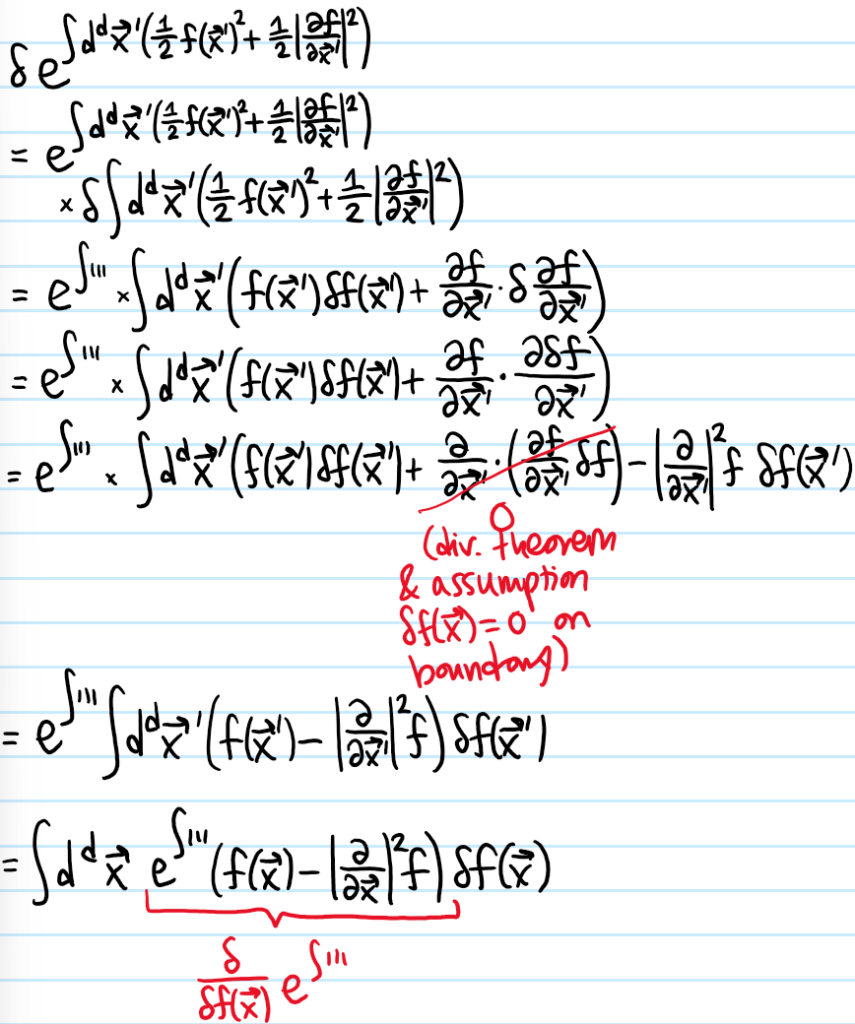
where \(\phi_*\) is the order parameter configuration minimizing the free energy \(F=F[\phi]\). In other words, \(\phi_*\) is a stationary point of \(F[\phi]\) so that the functional derivative \(\frac{\delta F}{\delta\phi^*}=0\) vanishes.
Landau mean field theory is the special case of this saddle-point approximation in which all fluctuations \(\phi_*=\phi_*(\textbf x)\) are completely ignored, yielding a homogeneous mean field order parameter.
Problem #\(3\): Explain why, as with many other functionals in physics (e.g. the action \(S[\textbf x]\)), the Landau-Ginzburg free energy functional \(F[\phi]\) must take the form:
\[F[\phi]=\int d^d\textbf x \mathcal F\left(\phi(\textbf x),\frac{\partial\phi}{\partial\textbf x},…\right)\]
Combining this with the saddle-point approximation in Solution #\(2\), what can one conclude?
Solution #\(3\): The presence of the integral \(\int d^d\textbf x\) simply reflects the extensive nature of the free energy \(F\), while the dependence of the integrand \(\mathcal F\) on \(\phi\) and its derivatives only reflects locality.
In the special case that the free energy density \(\mathcal F\) depends only on the field \(\phi(\textbf x)\) and its gradient \(\frac{\partial\phi}{\partial\textbf x}\) (but no higher derivatives), and it obeys suitable boundary conditions, one then has the usual Euler-Lagrange equations:
Problem #\(3\): Suppose that free energy density \(\mathcal F(\phi)\) of a particular system (e.g. the Ising ferromagnet) is taken (on locality, analyticity and suitable symmetry grounds) to be of the form:
where the phenomenological coupling constants \(\alpha_2,\alpha_4,\gamma\) each may carry some \(T\)-dependence, though as far as the study of second-order phase transitions at critical points is concerned, only the \(T\)-dependence \(\alpha_2(T)\sim T-T_c\) on the quadratic \(\phi^2\) term matters, and all that needs to be assumed about the other coupling constants is their signfor all temperatures \(T\), in this case \(\alpha_4,\gamma>0\). Show that in the subcritical regime \(T<T_c\), the \(\textbf Z_2\) symmetry \(F[-\phi]=F[\phi]\) of the theory is spontaneously broken via a bifurcation into \(2\) degenerate ground states (also called vacua in analogy with QFT) representing mean-field homogeneous/ordered phases/configurations \(\phi_*(\textbf x)=\phi_0\). Show that there is also a more interesting domain wall soliton:
that emerges upon imposing Dirichlet boundary conditions \(\lim_{x\to\pm\infty}\phi_*(\textbf x)=\pm\phi_0\) implementing a smooth transition interpolating between the two ground state phases \(\pm\phi_0\).
Solution #\(3\): The Euler-Lagrange equations for this particular free energy density \(\mathcal F\) yield a Poisson/Helmholtz-like (but nonlinear!) PDE for the on-shell field \(\phi_*(\textbf x)\):
Looking for a homogeneous ansatz \(\phi_*(\textbf x)=\phi_0\) yields the \(2\) degenerate ground states \(\phi_0=\sqrt{-\alpha_2/\alpha_4}\) with free energy density \(\mathcal F_0:=\mathcal F(\pm\phi_0)=-\alpha_2^2/4\alpha_4\) and corresponding Landau-Ginzburg free energy \(F_0:=F[\pm\phi_0]=L^d\mathcal F_0\) (putting the system in a box \([-L/2,L/2]^d\) to regularize the obvious IR divergence that would otherwise arise).
By contrast, reverting now to the Beltrami identity, assuming that \(\phi_*^{\text{DW}}(\textbf x)=\phi_*^{\text{DW}}(x)\) varies only along the \(x\)-direction, the PDE reduces to the nonlinear separable first-order ODE:
In particular, placing the domain wall at the origin \(x=0\) so that \(\phi(0)=0\), one obtains the soliton described (for a domain wall at some other location \(x_0\in\textbf R\), just translate \(x\mapsto x-x_0\) in the \(\tanh\) function). In particular; the width of the domain wall is \(\Delta x=\sqrt{-2\gamma/\alpha_2}\) which is pretty intuitive (c.f. the formula \(\omega_0=\sqrt{k/m}\) for a mass \(m\) on a spring \(k\)). Unlike the homogeneous ground states \(\pm\phi_0\), this domain wall soliton is a non-MF stationary point of the Landau-Ginzburg free energy functional \(F\).
Problem #\(4\): By definition, the ground state(s) of any system are global minima of its energy. In particular, it is clear that the domain wall soliton \(\phi_*^{\text{DW}}(x)\) is not a ground state, having free energy \(F[\phi_*^{\text{DW}}]>F_0\); precisely how much free energy \(\Delta F_{\text{DW}}:=F[\phi_*^{\text{DW}}]-F_0\) does it cost to create such a domain wall from a homogeneous ground state phase?
Solution #\(4\): Differential equations can (and should!) often be thought of as a dance/tension between conflicting characters. Even without doing any of the math in Solution #\(3\), it should be clear that the domain wall transition cannot happen instantaneously or the free energy cost \(\int d^d\textbf x\frac{\gamma}{2}\left(\frac{d\phi}{dx}\right)^2\) from the “kinetic” term would be too great, but neither can it proceed too slowly otherwise the free energy cost \(\int d^d\textbf x\left(\frac{\alpha_2}{2}\phi^2+\frac{\alpha_4}{4}\phi^4\right)\) from the “potential” term would be too great; the domain wall \(\phi_*^{\text{DW}}(x)\) must therefore strike a balance between these two free energy costs while satisfying the boundary conditions \(\lim_{x\to\pm\infty}\phi_*^{\text{DW}}(x)=\pm\phi_0\) (cf. the virial theorem in classical mechanics). In other words, \(0<\Delta x<\infty\).
(easy to forget, but remember one is working in the subcritical \(T<T_c\) regime where \(\alpha_2<0,\alpha_4>0\) so the potential term \(\frac{\alpha_2}{2}\phi^2+\frac{\alpha_4}{4}\phi^4\) is not positive semi-definite, in particular its minimum does not lie at \(\phi_0=0\) but rather has degenerate minima at \(\phi_0=\pm\sqrt{-\alpha_2/\alpha_4}\)! This means that anywhere \(\textbf x\in\textbf R^d\) that \(\phi_*^{\text{DW}}(\textbf x)\) strays too far away from the bottom of the potential wells at \(\pm\phi_0\) costs free energy, so for this reason the domain wall cannot take too long to climb over the hump between the two minima).
Indeed, the Beltrami identity quantifies this free energy balance and one can exploit it to quickly calculate the free energy of the domain wall soliton:
the latter term is recognized as just the free energy \(F_0=\int d^d\textbf x f_0=L^df_0\) of the ground state(s) so the excess free energy cost \(\Delta F_{\text{DW}}\) of creating the domain wall is (for \(L\gg\Delta x\)):
but the key point is that \(\Delta F_{\text{DW}}\sim L^{d-1}\) scales with the (hyper)area of the domain wall. Well actually, another important scaling to note is that \(\Delta F_{\text{DW}}\sim(-\alpha_2)^{3/2}\) which suggests that near criticality where \(\alpha_2\to 0\), the free energy cost \(\Delta F_{\text{DW}}\to 0\) of creating a domain wall also vanishes, while its width \(\Delta x\sim(-\alpha_2)^{-1/2}\) diverges. This suggests that domain walls become important near critical points.
Problem #\(5\): Working with the same Landau-Ginzburg system as above, estimate in \(d=1\) dimension the probability \(p_N\) that thermal fluctuations will spontaneously break the \(\textbf Z_2\) symmetry of the free energy \(F\) via the creation of \(N\ll L/\Delta x\) domain walls anywhere, and comment on the implication of this for the lower critical dimension \(d_{\ell}\) of this system.
Solution #\(5\): Because the ODE arising from the Beltrami identity was nonlinear, the superposition of a bunch of domain walls at different locations is not strictly speaking a stationary point of the free energy \(F\), but nonetheless one can sweep this under the rug and assume it is still an approximate solution provided the \(N\) domain walls are well-separated. In particular, this means their total free energy \(\approx N\Delta F_{\text{DW}}+F_0\) is also approximately additive. If one imagines discretizing the \(d=1\) line \([-L/2,L/2]\) into \(L/\Delta x\) bins each of width \(\Delta x\), then there are \(L/\Delta x\choose{N}\) choices for where to put the domain walls in (ignoring the fact that in some cases, they may not be so well-separated), so the probability of having any configuration of \(N\) domain walls is approximately:
where the sparse approximation has been used \(N\ll L/\Delta x\). Alternatively, normalizing with respect to the \(N=0\) “vacuum” probability \(p_0=e^{-\beta F_0}/Z\):
Importantly, in \(d=1\) domain walls are free since \(\Delta F_{\text{DW}}\sim L^{1-1}=L^0\). So all the \(L\)-dependence in the expression above for \(p_N/p_0\) is contained in the entropic factor \((L/\Delta x)^N/N!\) and shows that as one takes the infinite system limit \(L\to\infty\), the probability \(p_N/p_0\) receives no exponential suppression from the \(e^{-N\beta\Delta F_{\text{DW}}}\) and instead grows unbounded. The probability that thermal fluctuations produce an even number \(N\in 2\textbf N\) of domain walls is:
and since \(\lim_{\varphi\to\infty}\tanh\varphi=1\), these two probabilities both approach the same \(e^{Le^{-\beta\Delta F_{\text{DW}}}/\Delta x}p_0/2\) as \(L\to\infty\).
More generally, any Landau-Ginzburg theory with a discrete symmetry (like the \(\textbf Z_2\) symmetry of this particular \(F\)) will possess a bunch of disconnected, degenerate ground states/vacua (like the \(\phi(\textbf x)=\pm\phi_0\) in this case) that spontaneously break that discrete symmetry, and all have \(d_{\ell}=1\) because there is very high probability that thermal fluctuations will proliferate domain walls that toggle between the degenerate ground states, preventing ordered phases from forming. Hence for instance the Ising model has no phase transitions in \(d=1\).
Problem #\(6\):
Solution #\(6\):
Problem #\(7\):
Solution #\(7\):
Note that if one does not work in natural units, then the heat capacity is instead \(C=k_B\beta^2\frac{\partial^2\ln Z}{\partial\beta^2}\) so all specific heat capacities should come with an additional factor of \(k_B\).
Problem #\(8\):
Solution #\(8\):
Problem #\(9\):
Solution #\(9\):
(NEED TO COME BACK TO THIS QUESTION!)
Problem #\(10\): Describe the quadratic approximation to the Landau-Ginzburg free energy density \(\mathcal F\) governing a \(\textbf Z_2\)-symmetric system/theory (e.g. Ising ferromagnet) described by a single, real scalar order parameter \(\phi\) in the absence of any external coupling \(E_{\text{ext}}=0\).
Solution #\(10\): On LAS (locality, analyticity, symmetry) grounds, the exact free energy density \(\mathcal F\) that knows about the all detailed microscopic physics must take the phenomenological form:
where in principle there are also coupling constants for \(\phi^6,\phi^5\biggr|\frac{\partial\phi}{\partial\textbf x}\biggr|^2\biggr|\frac{\partial}{\partial\textbf x}\biggr|^2\phi\) etc. though not for couplings like \(\phi^3\) or \(1/\phi^2\). In addition, one also has to import from mean-field theory the assumption that \(\alpha_2\sim T-T_c\) (i.e. \(\alpha_2\to 0\) as \(T\to T_c\) in a linear/critical exponent \(1\) manner) and that \(\gamma,\alpha_4>0\) for all \(T\) in a neighbourhood of \(T_c\).
The quadratic approximation to \(\mathcal F\) looks slightly different depending on whether one is working in the supercritical \(T>T_c\) regime (where \(\alpha_2(T)>0\)) or the subcritical \(T<T_c\) regime (where \(\alpha_2(T)<0\)).
In the supercritical \(T>T_c\) regime, the quadratic approximation does what it sounds like, in fact drop not only all quartic, sextic, octic, decic, etc. couplings like \(\phi^4,\biggr|\frac{\partial\phi}{\partial\textbf x}\biggr|^{22}\) but even quadratic couplings containing Laplacians, third derivatives, biharmonics, and all higher-derivative couplings. So at \(T>T_c\), this amounts to keeping only \(2\) couplings, a “kinetic” coupling \(\frac{\gamma}{2}\biggr|\frac{\partial\phi}{\partial\textbf x}\biggr|^2\) and a “Hookean quadratic potential” coupling \(\frac{\alpha_2}{2}\phi^2\):
where the fluctuation \(\delta\phi(\textbf x):=\phi(\textbf x)-\langle\phi(\textbf x)\rangle\). This is simply because, at \(T>T_c\), \(\langle\phi(\textbf x)\rangle=0\) vanishes homogeneously (from mean-field theory).
By contrast, in the subcritical \(T<T_c\) regime, the quadratic approximation consists of \(2\) separate approximation steps:
Step #\(1\): Keep not only the zeroth and first-order quadratic couplings that were retained in the supercritical \(T>T_c\) case, but also keep the quartic \(\phi^4\) coupling:
The reason for this is that for \(T<T_c\), \(\alpha_2(T)<0\) so the free energy density \(\mathcal F(\phi)=-\frac{|\alpha_2|}{2}\phi^2+…\) would be unbounded from below, yielding an unstable theory. By including the quartic coupling, one instead has \(2\) degenerate \(\textbf Z_2\) symmetry breaking homogeneous ordered phases \(\phi(\textbf x)=\pm\phi_0\) with \(\phi_0=\sqrt{-\alpha_2/\alpha_4}\).
However, beyond the presence of \(\alpha_4\) in \(\phi_0\), one would otherwise like to remove all other vestiges of it in \(\mathcal F\) in order to get a more quadratic-looking free energy density like in the \(T>T_c\) case. Thus:
Step #\(2\): Insert the “Reynolds decomposition” \(\phi=\phi_0+\delta\phi\) into \(\mathcal F\) and notice that the term linear in \(\delta\phi\) vanishes because \(\phi_0\) is on-shell:
where the cubic and quartic couplings \(O(\delta\phi^3)=2\alpha_4\phi_0\delta\phi^3+\frac{\alpha_4}{2}\delta\phi^4\) at the level of the fluctuations \(\delta\phi\) from the mean field \(\phi_0\) are assumed negligible in this second step of the quadratic approximation for \(T<T_c\). Finally, note that the constant term \(\mathcal F[\phi_0]\) would drop out when differentiating \(\ln Z\) to compute Boltzmannian cumulants, so can safely be omitted.
In this way, the name “quadratic approximation” is justified because both the \(T>T_c\) and \(T<T_c\) cases can be unified by writing the free energy as:
Problem #\(11\): Working within the quadratic approximation to the free energy density \(\mathcal F\) outlined in Solution #\(11\), compute the partition function \(Z\).
Solution #\(11\): This is pretty much the only case where the path integral underlying \(Z\) can be computed analytically thanks to the fact that Gaussian integrals are straightforward to do. Here is a sketch of the computation:
Step #\(1\): The free energy \(F=\int d^d\textbf x\mathcal F(\delta\phi)\) is certainly extensive so one must add up \(\int\) the chunks of free energy \(d^d\textbf x\mathcal F(\delta\phi)\) due to fluctuations \(\delta\phi\) of the order parameter \(\phi\) at each point \(\textbf x\in\textbf R^d\) in space (or \(\textbf x\in V\subset\textbf R^d\) in some suitably large volume). But conceptually, some of these fluctuations might be more short-range, rapid oscillations across \(\textbf x\), while others may be more long-range, slow envelopes. Nonetheless, it should be intuitively clear that, rather than taking the local approach of stepping through each \(\textbf x\in\textbf R^d\) and adding up the energies of all fluctuations at that point \(\textbf x\), one can take a more global approach of adding up the energies of all fluctuations across the entire space \(\textbf R^d\) that have a given wavelength \(\lambda\) (or equivalently wavenumber \(k=2\pi/\lambda\)), and stepping through all possible wavelengths, from the long (“IR”) wavelengths all the way down to the short (“UV”) wavelengths. This intuitive picture can of course be formalized by explicitly writing \(\delta\phi(\textbf x)\) as a superposition of plane wave excitations:
which uses the fact that for \(\delta\phi(\textbf x)\in\textbf R\), the Fourier transform satisfies \(\delta\phi_{-\textbf k}=\delta\phi^{\dagger}_{\textbf k}\). By viewing the system as having some large but finite volume \(V\), one can replace on dimensional grounds:
where \(\sum_{\textbf k}\) means over all \(\textbf k=\frac{2\pi}{L}\textbf n\) for \(\textbf n\in\textbf Z^d\) since these are the only wavevectors compatible with periodic boundary conditions on \(\delta\phi(\textbf x)\) in a box \([-L/2,L/2]^d\) of volume \(V=L^d\). Put another way, it reduces Plancherel’s theorem for the Fourier transform to Parseval’s theorem for Fourier series (since \(\delta\phi(\textbf x)\) is now \(L\)-periodic in all \(d\) dimensions).
Finally, the existence of the plane wave basis also allows one to “rigorously” define the measure \(\mathcal D\phi=\mathcal D\delta\phi\) in the path integral for \(Z=\int\mathcal D\delta\phi e^{-\beta F[\delta\phi]}\). Intuitively, the path integral \(\int\mathcal D\delta\phi\) wants to sum over all possible fluctuations \(\delta\phi\) of the field about the mean field. But the Fourier transform allows one to explicitly parameterize this abstract space! Simply integrate over all possible choices of the “Fourier knobs/coefficients” \(\phi_{\textbf k}\) which can span any fluctuation \(\delta\phi\):
where the product \(\prod_{\textbf k}\) is over the same countably infinite lattice of \(\textbf k\)-wavevectors as the earlier sum \(\sum_{\textbf k}\) (actually, strictly speaking, one should only take the product over half of the entire \(\textbf k\)-space, for instance imposing \(k_x>0\). This is because if \(\delta\phi_{\textbf k}\in\textbf C\) is already known for some \(\textbf k\), then \(\delta\phi_{-\textbf k}\) is also automatically known by virtue of the reality criterion \(\delta\phi_{-\textbf k}=\delta\phi^{\dagger}_{\textbf k}\), cf. \(\sin(kx)=\frac{1}{2i}e^{ikx}+?e^{-ikx}\) where, knowing that \(\sin(kx)\in\textbf R\), one can immediately conclude that \(?=(\frac{1}{2i})^{\dagger}=-\frac{1}{2i}\). So \(\delta\phi_{\textbf k}\) and \(\delta\phi_{-\textbf k}\) are not independent knobs (imagine a “complex conjugation gear” between them), but the path integral \(\int\mathcal D\delta\phi\) only wants to integrate over independent degrees of freedom since double-counting the same fluctuation is obviously not desired. That being said, this only leads to a factor of \(2\) discrepancy which doesn’t affect any physical quantities, and the measure \(\mathcal D\delta\phi\) is only defined up to some “normalization” anyways).
At this point one writes \(|\delta\phi_{\textbf k}|^2=\Re^2\delta\phi_{\textbf k}+\Im^2\delta\phi_{\textbf k}\) and decouples all the Gaussian integrals to obtain the final result for \(Z\):
Problem #\(12\): Using this \(Z\), and making the specific assumption that \(\alpha_2(T)=k_B(T-T_c)\) and that \(\gamma\) is independent of \(T\), compute the specific heat capacity \(c\) of this Landau-Ginzburg system in the supercritical \(T>T_c\) regime.
where the \(\frac{k_B}{2}\times 1\) part reflects equipartition of quadratic degrees of freedom and is simply due to the \(\beta\) temperature dependence in \(e^{-\beta F}\) (fluctuation-dissipation theorem?). By contrast, the other terms are additional contributions to the heat capacity arising from the \(T\)-dependence in \(F\) instead, specifically in \(\mu^2=k_B(T-T_c)\).
Problem #\(13\): Clearly, the specific heat capacity \(c\) as it’s currently written suffers from a \(|\textbf k|\to\infty\) UV divergence, since it is that part of the integrand that causes the integral to diverge to \(\infty\). What should one make of this?
Solution #\(13\): To regularize this UV divergence, one has to impose a UV cutoff \(k^*\) with the property that the Fourier transform \(\delta\phi_{\textbf k}\) is only supported for \(|\textbf k|\leq k^*\) in the \(k^*\)-ball. This UV cutoff should be chosen so that \(k^*\sim 1/\Delta x\), with \(\Delta x\) being the lattice spacing of some underlying microscopic structure which has been coarse-grained away. By implementing a UV cutoff, the specific heat capacity \(c\) is made finite:
where the (hyper)surface area of the unit \(d-1\)-sphere is \(|S^{d-1}|=2\pi^{d/2}/\Gamma(d/2)\).
(aside: to prove this, notice that the \(d\)-dimensional isotropic Gaussian integral \(\int_{\textbf x\in\textbf R^d} d^d\textbf x e^{-|\textbf x|^2}\) evaluates to \(\pi^{d/2}\) when separated in Cartesian coordinates, or equivalently \(|S^{d-1}|\int_0^{\infty}d|\textbf x||\textbf x|^{d-1}e^{-|\textbf x|^2}\) in spherical coordinates. The latter integral can then be massaged into the form of a gamma function \(\Gamma(d/2)/2\) via the substitution \(z:=|\textbf x|^2\)).
For some small dimensions \(d=1,2,3,4,5\), the \(2\) integrals can be evaluated analytically, with results compiled in the table below:
or in hindsight many of these can be written more compactly via the (yet unmotivated) correlation length \(\xi:=\sqrt{\gamma}/\mu\).
Problem #\(14\): Using the results of Problem #\(14\), comment on how \(c\) behaves in various dimensions \(d\) as one approaches the critical point \(T\to T_c^+\) from above (since the results above were all computed within the supercritical \(T>T_c\) regime, though the analysis is the same in the subcritical \(T<T_c\) regime).
Solution #\(14\): As \(T\to T_c^+\), the quadratic coupling constant \(\mu^2\to 0\) vanishes. For \(d\geq 5\), both of the integrals above converge to a finite value determined by the choice of UV cutoff wavenumber \(k^*\), so \(c\) is also finite, and more precisely \(c\sim(k^*)^{d-2}\) from the first integral. For \(d=4,3\), only the first integral diverges while the second one converges, whereas for \(d=2,1\), both integrals diverge. For \(d\leq 3\), this divergence goes like \(c\sim\mu^{d-4}\) whereas for \(d=4\) it is a logarithmic divergence \(c\sim\ln\mu\) (both of these being determined in this case by the second integral).
In the case \(d\leq 3\), since \(\mu^2\sim T-T_c\) as \(T\to T_c^+\), this implies that \(c\sim (T-T_c)^{(d-4)/2}\) but in general the critical exponent \(\alpha\) is defined by the property that \(c\sim |T-T_c|^{-\alpha}\). Although this analysis was only for \(T>T_c\), one can check that for \(T<T_c\) one would have mirror behavior, so this analysis shows that, at least for \(d\leq 3\), the critical exponent is \(\alpha=2-d/2\). Thus, the contribution of fluctuations causes the critical exponent to differ from the mean-field prediction \(\alpha=0\).
Problem #\(15\): At each \(\textbf x\in\textbf R^d\), one can associate a continuous random variable \(\phi(\textbf x)\) which draws an order parameter configuration \(\phi\) from a thermal Boltzmann distribution \(p[\phi]=e^{-\beta F[\phi]}/Z\) and returns the evaluation of \(\phi\) at \(\textbf x\). Given two arbitrary positions \(\textbf x,\textbf x’\in\textbf R^d\), each giving rise to its own random variable \(\phi(\textbf x),\phi(\textbf x’)\), define the connected \(2\)-point correlation propagator \(\langle\delta\phi(\textbf x)\delta\phi(\textbf x’)\rangle\) between \(\textbf x,\textbf x’\).
Solution #\(15\): The connected \(2\)-point correlation propagator is simply the cross-covariance of the random variables \(\phi(\textbf x),\phi(\textbf x’)\). It is thus related to the cross-correlation \(\langle\phi(\textbf x)\phi(\textbf x’)\rangle\) between \(\textbf x,\textbf x’\) and their individual expected values \(\langle\phi(\textbf x)\rangle,\langle\phi(\textbf x’)\rangle\) by the usual parallel axis theorem (sort of…):
(comment: the \(1\)st and \(3\)rd functionals are local whereas the \(2\)nd functional one is nonlocal).
Solution #\(16\): Functions \(f(\textbf x)\) are like \(\infty\)-dimensional vectors whose components are indexed not by a discrete label \(i\) but rather by a continuous label \(\textbf x\in\textbf R^d\); one may as well write \(f_{\textbf x}\) or \(\langle\textbf x|f\rangle\) rather than \(f(\textbf x)\) to stress this point. The functional derivative is then conceptually no different from a partial derivative with respect to one of these infinitely many components \(f(\textbf x)\) of \(f\) and just ends up returning a vanilla function of \(\textbf x\).
Just as for a function \(F(f_1,f_2,…)\) of some real variables \(f_1,f_2,…\in\textbf R\) one has the total differential:
\[dF=\sum_i\frac{\partial F}{\partial f_i}df_i\]
So simply replacing the sum by an integral \(\sum_i\mapsto\int d^d\textbf x\), the functional derivative of a functional \(F[f]\) with respect to the variable \(f(\textbf x)\) is defined by requiring:
where typically one takes \(\delta\phi(\textbf x)=0\) for \(\textbf x\) on the boundary of the domain of integration in \(\textbf R^d\).
Notice that functional derivatives are much easier to compute than functional integrals, reflecting the general trend from single-variable calculus that differentiation is easier than integration. In particular, for functionals which are either directly (as in the \(1\)st and \(2\)nd examples) or indirectly (as in the \(3\)rd example) related to some integral of the function, functional differentiation just boils down to partial differentiation of the integrand. Keeping in mind that \(\delta f(\textbf x)=0\) for \(\textbf x\in\partial\), the key identity in this regard, generalizing the Euler-Lagrange equations, is:
seems intuitively clear (cf. \(\langle\textbf x’|\textbf x\rangle=\delta^3(\textbf x-\textbf x’)\) in nonrelativistic quantum mechanics), but how does one go about “rigorously” interpreting and proving it?
Solution #\(17\): The idea, mentioned before, is to view \(f(\textbf x’)=\text{eval}_{\textbf x’}[f]\) as an evaluation functional so that it really can be interpreted as a functional derivative. Then, express the evaluation functional in the integral form that one is most comfortable with by convolving with a delta:
\[f(\textbf x’)=\int d^d\textbf x f(\textbf x)\delta^d(\textbf x-\textbf x’)\]
So the result follows from the considerations in Solution #\(16\).
Problem #\(18\): In general, what are the dimensions of the functional derivative \(\frac{\delta F}{\delta f}\)? Look back at both Problems #\(16,17\) and check this.
Solution #\(18\): Although one is used to intuitively reading off dimensions from regular derivatives like \([\partial f/\partial x]=[f]/[x]\), for functional derivatives the “densitized” nature of the continuum \(d^d\textbf x\) means that actually:
which in particular is not equal to the naive \([F]/[f]\) (unless \(d=0\) which is boring). This is consistent with the functional derivatives in both Solutions #\(16,17\).
Problem #\(19\): Show that by “applying an external magnetic field” \(E_{\text{ext}}(\textbf x)\) to the system, one has for the original exact Landau-Ginzburg free energy bifunctional \(F[\phi,E_{\text{ext}}]\) (i.e. not the quadratic approximation \(F=F[\delta\phi]\)) the functional derivatives:
Solution #\(19\): The Zeeman coupling is linear, so mathematically it is a chemist’s Legendre transform of the free energy density \(\mathcal F\) from \(\phi\to E_{\text{ext}}\):
Proving the \(1\)st identity concerning \(\langle\phi(\textbf x)\rangle\) is easy, and it can be directly substituted into the \(2\)nd identity to give:
where at the end one can also turn off \(E_{\text{ext}}(\textbf x)=0\) to get the ensemble average and \(2\)-point correlator in the original \(\textbf Z_2\) theory.
Problem #\(20\): Using the results of Solution #\(17\), show that, reverting back to the quadratic approximation of \(\mathcal F\):
where \(G(\textbf x)\) is almost a stationary point of the quadratic free energy \(F\) through being the fundamental Green’s function of the Helmholtz operator \(\mu^2-\gamma\biggr|\frac{\partial}{\partial\textbf x}\biggr|^2\) on \(\textbf R^d\):
Solution #\(20\): Essentially the same as Solution #\(11\) except that need to first complete the square in the free energy (which uses the reality of the magnetic field \(E_{\text{ext}}(\textbf x)\in\textbf R\Leftrightarrow E_{\text{ext}}^{-\textbf k}=\left(E_{\text{ext}}^{\textbf k}\right)^{\dagger}\))
and then do the Gaussian path integral to get the original partition function (when \(E_{\text{ext}}=0\)) with an additional Plancherelian contribution from \(E_{\text{ext}}\neq 0\):
Or, substituting \(E_{\text{ext}}^{\textbf k}=\int d^d\textbf x E_{\text{ext}}(\textbf x)e^{-i\textbf k\cdot\textbf x}\) to revert from \(\textbf k\mapsto\textbf x\) (in anticipation that one would like to take functional derivatives with respect to \(E_{\text{ext}}(\textbf x)\)):
From here, the functional derivatives are straightforward to take (and only the \(2\)nd term above matters):
(aside: it seems that \(E_{\text{ext}}(\textbf x)\) can be interpreted as some kind of fluctuation distribution which, upon convolving with the \(2\)-point correlator, solves the inhomogeneous Helmholtz equation:
where \(r:=|\textbf x-\textbf x’|\) the identity \(\frac{d-3}{2}+\frac{d-1}{2}=d-2\) ensures dimensional consistency and is a good way to remember it (and indeed the \(d-2\) follows on dimensional analysis grounds).
Solution #\(22\): The derivation involves a clever saddle-point approximation:
Problem #\(23\): What are the critical exponents \(\nu,\eta\) in the mean-field, quadratic approximation to the full Landau-Ginzburg theory?
Solution #\(23\): The critical point is defined to be where the quadratic coupling \(\mu^2=0\) vanishes. So get any kind of critical exponent, this always just means: write down a formula for the quantity of interest in terms of \(\mu\sim |T-T_c|^{1/2}\). For the correlation length, this is trivial:
so \(\nu=1/2\). In particular, as \(T\to T_c\), the correlation length diverges \(\xi\to\infty\). This also means that at the critical point, the only relevant regime in the Ornstein-Zernicke \(2\)-point correlator is \(r\ll\xi\to\infty\), so:
Problem #\(24\): Using the Ginzburg criterion, rationalize why the upper critical dimension \(d_c=4\) for the Ising model.
Solution #\(24\): Conceptually, the Ginzburg criterion is a common sense idea. It says that mean-field theory has sensible things to say about the critical point \(T\to T_c\) iff:
\[\text{fluctuations about mean field}\ll\text{mean field itself}\]
or, mathematically (integrating only within a \(\xi\)-ball due to the exponentially-decaying Ornstein-Zernicke correlation for \(|\textbf x|>\xi\)):
But at the critical point \(\beta\gamma\to\beta_c\gamma_c\) which is just finite number…so in order for the left side of the equality to also remain bounded as \(T\to T_c\), require:
\[\nu(d-2)\geq 2\beta\]
Using the mean-field exponents \(\beta=\nu=1/2\), this amounts to constraining \(d\geq 4=d_c\). This may seem a bit sketchy given that the mean-field exponents for \(\beta,\nu\) were used in the Ginzburg criterion to show that mean-field theory is consistent. Rather, it just means that MFT is self-consistent. On the other hand, for \(d<4\), MFT literally predicts its own demise!
Solution #\(1\): In words, the Poincaré group is the isometry group of Minkowski spacetime \(\textbf R^{1,3}\). Mathematically, it is the semidirect product \(\textbf R^{1,3}⋊O(1,3)\) of the normal subgroup \(\textbf R^{1,3}\) of spacetime translations with the Lorentz subgroup \(O(1,3)\) of rotations, Lorentz boosts, parity, and time reversal:
The reason the Poincaré group is a semidirect product rather than simply a direct product \(\textbf R^{1,3}\times O(1,3)\) is that spacetime translations and Lorentz transformations talk to each other via the Poincaré group’s composition rule:
Problem #\(2\): With the exception of parity and time reversal, all symmetries of the Poincaré group can be implemented continuously:
where the green box of proper, orthochronous Poincaré transformations is the connected component of the identity \(1\) and the only one of the \(4\) connected components which by itself comprises a subgroup of the Poincaré group. Among the \({4}\choose{2}\)\(=6\) pairs of connected components one can join together, the \(2\) pairs:
are the only subgroups of the Poincaré group \(\textbf R^{1,3}⋊O(1,3)\). Anyways, this digression is just to say that, modulo the Klein \(4\)-group quotient structure \(\{1,\Pi,\Theta,\Pi\Theta\}\), the proper, orthochronous Poincaré group \(\textbf R^{1,3}⋊SO^+(1,3)\) is a Lie group and hence can be studied via its Lie algebra. Classify fully the structure of this so-called Poincaré algebra.
Solution #\(2\): Consider spacetime translations \(\Delta X\in\textbf R^{1,3}\) first. It is clear that:
where \(\Delta X\cdot\frac{\partial}{\partial X}=\Delta X^{\mu}\partial_{\mu}\) is a Lorentz scalar. Although there’s nothing quantum mechanical about what is being done here, for sake of comparison one can artificially introduce \(\hbar\) and define the generator of spacetime translations \(P:=-i\hbar\frac{\partial}{\partial X}\Leftrightarrow P_{\mu}=-i\hbar\partial_{\mu}\) so that a general spacetime translation would be given by the infinite-dimensional unitary representation \(e^{-i\Delta X\cdot P/\hbar}\). Since spacetime translations are abelian, the algebra is simply characterized by \([P_{\mu},P_{\nu}]=0\).
Considering proper, orthochronous Lorentz transformations \(\Lambda\in SO^+(1,3)\) next, recall that membership in \(O(1,3)\) means that:
So if one substitutes \(\Lambda=1+\omega\Leftrightarrow \Lambda^{\mu}_{\space\space\nu}=\delta^{\mu}_{\space\space\nu}+\omega^{\mu}_{\space\space\nu}\) for infinitesimal \(\omega\), one finds that any such generator \(\omega\in\frak{so}^+\)\((1,3)\) must be antisymmetric:
which is unsurprising considering \(SO^+(1,3)\) is similar to \(SO(4)\). Thus, one can adapt the obvious \(\frak{so}\)\((4)\) basis of \(6\) antisymmetric generators to the Lorentz Lie algebra \(\frak{so}\)\(^+(1,3)\). There are various notations with which one can express these \(6\) generators:
More Intuitive Notation: One has \(3\) generators \(\textbf J:=(J_1,J_2,J_3)\) for rotations and \(3\) generators \(\textbf K:=(K_1,K_2,K_3)\) for Lorentz boosts such that by definition a rotation through angular displacement \(\Delta\boldsymbol{\phi}\) is given by \(e^{-i\Delta\boldsymbol{\phi}\cdot\textbf J/\hbar}\) and a Lorentz boost through rapidity \(\Delta\boldsymbol{\varphi}\) is given by \(e^{-i\Delta\boldsymbol{\varphi}\cdot\textbf K/\hbar}\). One can kind of “cheat” using one’s prior knowledge about how macroscopic Lorentz transformation matrices \(\Lambda\) look in the case of rotations or Lorentz boosts about various axes, “infinitesimalize” them, and extract the corresponding generator. For example, for a rotation about the \(z\)-axis, as \(\Delta\phi\to 0\) one expects to \(\mathcal O(\Delta\phi)\):
and similarly for \(K_2,K_3\). In light of these matrix representations for the Lorentz Lie algebra generators, one can directly compute their commutation relations:
\[[J_i,J_j]=i\hbar\varepsilon_{ijk}J_k\]
\[[J_i,K_j]=i\hbar\varepsilon_{ijk}K_k\]
\[[K_i,K_j]=-i\hbar\varepsilon_{ijk}J_k\]
where the last commutator expresses (via the BCH formula) the counterintuitive phenomenon of Wigner rotation associated with non-collinear \(i\neq j\) Lorentz boosts.
Less Intuitive Notation: The cross product on \(\textbf R^3\) realizes a representation of the rotation algebra \(\frak{so}\)\((3)\) given by assigning each antisymmetric tensor \(\omega\in\frak{so}\)\((3)\) to the unique vector \(\boldsymbol{\omega}\in\textbf R^3\) such that \(\omega\textbf x=\boldsymbol{\omega}\times\textbf x\) for all \(\textbf x\in\textbf R^3\). More explicitly:
Or in indices, \(\omega_{ij}=-\varepsilon_{ijk}\omega_k\) or, inverting by contraction with a suitable Levi-Civita symbol, one has the equivalent form \(\omega_k=-\frac{1}{2}\varepsilon_{ijk}\omega_{ij}\). Here, the vector \(\boldsymbol{\omega}\) is arguably more intuitive than the tensor \(\omega\) even though both contain exactly the same information.
In precisely this same spirit, one can take the more intuitive “vector” generators \(\textbf J,\textbf K\) for rotations and Lorentz boosts and convert them into the equivalent but less intuitive form of a \(4\times 4\) matrix, each of whose \(16\) elements is itself a \(4\times 4\) matrix (one could even think of this as a \(16\times 16\) matrix if one so desired). That is, it is typical to define:
where \(0\leq \mu,\nu,\rho,\sigma\leq 3\) are all spacetime indices (this is partly the reason for introducing this less intuitive representation of the Lorentz algebra because it puts space and time on more equal footing in this compact expression). This is related to the more intuitive representation above by:
One can then compute the Lorentz algebra in a single sweep:
Lowering the \(\nu\) index with the metric (it’s more useful to have it like this since Lorentz transformations have a conventionally NW-SE index structure \(\Lambda^{\mu}_{\space\space\nu}\) and one is anticipating generating these by exponentiating linear combinations of these generators):
so that an arbitrary Lorentz algebra element \(\omega\in\frak{so}^+\)\((1,3)\) (not necessarily infinitesimal anymore) is some linear combination of the \(6\) generators \(\mathcal M^{\rho\sigma}\in\frak{so}^+\)\((1,3)\) with real coefficients \(\Delta\Phi_{\rho\sigma}\in\textbf R\) quantifying the extent of a rotation or Lorentz boost (they are related to the earlier more intuitive representation by \(\Delta\phi_i=\) and \(\Delta\varphi_i=\)):
where the factor of \(1/2\) is to compensate for double-counting (since both \(\Delta\Phi_{\sigma\rho}=-\Delta\Phi_{\rho\sigma}\) and \(\mathcal M^{\sigma\rho}=-\mathcal M^{\rho\sigma}\) are antisymmetric in their indices \(\rho,\sigma\)) (explicitly write out \(\Phi\) to have \(\textbf J,\textbf K\) entries inside).
Finally, spacetime translations talk with Lorentz transformations (recall the proper, orthochronous Poincaré group is given by a semi-direct product \(\textbf R^{1,3}⋊SO^+(1,3)\)), so to fully specify the Poincaré algebra, one also has to figure out how the generators \(P:=(H/c,\textbf P)\) of \(\textbf R^{1,3}\) talk with the generators \(\textbf J,\textbf K\) of \(\frak{so}^+\)\((1,3)\), not just how they talk within their own Lie subalgebras.
It turns out one can concisely summarize all the remaining commutation relations within the Poincaré algebra in the more intuitive form:
Problem #\(3\): Motivate the general definition of a Clifford algebra in mathematics, state the anticommutation relations of the specific Clifford algebra \(\text{Cl}_{1,3}(\textbf R)\), and state the chiral/Weyl representation of \(\text{Cl}_{1,3}(\textbf R)\).
Solution #\(3\): Given a vector space \(V\) over a field \(F\), a quadratic form \(Q:V\to F\) is any function with \(2\) properties:
\(Q(\lambda\textbf v)=\lambda^2Q(\textbf v)\) for all vectors \(\textbf v\in V\) and scalars \(\lambda\in F\).
The function \(\langle\space|\space\rangle:V\times V\to F\) defined by \(\langle\textbf v|\textbf w\rangle:=\frac{1}{2}(Q(\textbf v+\textbf w)-Q(\textbf v)-Q(\textbf w))\) is a bilinear form (called the polarization of \(Q\)).
Note that \(Q\) and \(\langle\space|\space\rangle\) contain exactly the same information, since one can also invert \(Q(\textbf v)=\langle\textbf v|\textbf v\rangle\). A general quadratic form on Euclidean space \(\textbf R^n\) is of the form \(Q(\textbf v):=\textbf v^Tg\textbf v\) (where without loss of generality one can take \(g^T=g\) to be symmetric) whose associated symmetric bilinear form is \(\langle\textbf v|\textbf w\rangle=(\textbf v^Tg\textbf w+\textbf w^Tg\textbf v)/2\). In particular, when \(g=1\) is the standard metric on Euclidean space, then \(\langle\textbf v|\textbf w\rangle=\textbf v\cdot\textbf w\) coincides with the usual dot product.
Given a quadratic space \((V,F,Q)\), one can construct from this the Clifford algebra \(\text{Cl}(V,F,Q)\) by starting with the tensor algebra \(\oplus_{k=0}^{\infty}V^{\otimes k}\) of \(V\) and quotienting it by the relation \(\textbf v^2:=\textbf v\otimes\textbf v=Q(\textbf v)1_V\) for all \(\textbf v\in V\). From this, it follows as a corollary that more generally, for any two vectors \(\textbf v,\textbf w\in V\):
where in physics contexts the tensor product \(\textbf v\otimes\textbf w\) is often abbreviated to just \(\textbf v\textbf w\) and called the geometric product. Furthermore, since this anticommutator \(\{\textbf v,\textbf w\}\) is bilinear, it may be completely specified by finding a basis \(\textbf e_i\) of \(V\) and simply specifying the value of \(\{\textbf e_i,\textbf e_j\}\) for all pairs of basis vectors \(\textbf e_i,\textbf e_j\). Returning to the example of \(\textbf R^n\) with the standard metric, if one chooses an orthonormal basis \(\hat{\textbf e}_i\cdot\hat{\textbf e}_j=\delta_{ij}\), then the Clifford algebra is simply characterized by \(\{\hat{\textbf e}_i,\hat{\textbf e}_j\}=2\delta_{ij}1\). More explicitly, the \(\hat{\textbf e}_i\) all anticommute with each other and each squares to the identity \(\hat{\textbf e}^2_i=1\).
In \(\textbf R^2\), picking an orthonormal basis \(\hat{\textbf e}_1,\hat{\textbf e}_2\), although a general element of the Clifford algebra \(\text{Cl}_2(\textbf R)\) is formally:
The anticommutation relations of the Clifford algebra allow one to substantially reduce the number of degrees of freedom e.g. \(\hat{\textbf e}_1\hat{\textbf e}_1=\hat{\textbf e}_2\hat{\textbf e}_2=1\) and \(\hat{\textbf e}_1\hat{\textbf e}_2=-\hat{\textbf e}_2\hat{\textbf e}_1\)). All higher-order multivectors also reduce to either a scalar, a vector, or a bivector, e.g. \(\hat{\textbf e}_1\hat{\textbf e}_2\hat{\textbf e}_1=-\hat{\textbf e}_1\hat{\textbf e}_1\hat{\textbf e}_2=-\hat{\textbf e}_2\). So in fact, a general element of the Clifford algebra \(\text{Cl}_2(\textbf R)\) is simply spanned by \(4\) generators:
While the scalars and vectors \(1^2=\hat{\textbf e}_1^2=\hat{\textbf e}_2^2=1\) all square to the identity, the bivector \((\hat{\textbf e}_1\hat{\textbf e}_2)^2=-1\) squares to minus the identity! This is reminiscent of the identity \(i^2=-1\), where \(i=\sqrt{-1}\) is the imaginary unit of \(\textbf C\).
In \(\textbf R^3\), now with an orthonormal basis \(\hat{\textbf e}_1,\hat{\textbf e}_2,\hat{\textbf e}_3\), a general element of the Clifford algebra \(\text{Cl}_3(\textbf R)\) is parameterized by \(8\) real degrees of freedom (extrapolating, it should be clear by Pascal’s triangle that \(\dim\text{Cl}_{n}(\textbf R)=2^n\)):
note that \(\text{Cl}_3(\textbf R)\) can be explicitly represented by the \(3\) Pauli matrices \(\{\sigma_i,\sigma_j\}=2\delta_{ij}1\). In addition, the bivectors \((\hat{\textbf e}_1\hat{\textbf e}_2)^2=(\hat{\textbf e}_2\hat{\textbf e}_3)^2=(\hat{\textbf e}_1\hat{\textbf e}_3)^2=-1\) all square to minus the identity while \(\hat{\textbf e}_1\hat{\textbf e}_2\hat{\textbf e}_2\hat{\textbf e}_3\hat{\textbf e}_3\hat{\textbf e}_1=-1\), reminiscent of the defining relations \(i^2=j^2=k^2=ijk=-1\) of the quaternions \(\textbf H\) (H for “Hamilton”).
In special relativity, Minkowski spacetime \(\textbf R^{1,3}\) is a real vector space that naturally comes with a quadratic form \(Q(X):=X^T\eta X\) induced by the Minkowski metric \(g=\eta=\text{diag}(1,-1,-1,-1)\). Its associated \(16\)-dimensional Clifford algebra \(\text{Cl}_{1,3}(\textbf R)\) is therefore subject to the anticommutation relations:
\[\{\gamma^{\mu},\gamma^{\nu}\}=2\eta^{\mu\nu}1\]
for which one representation (and it turns out the only \(4\)-dimensional irreducible representation up to unitary similarity) is the chiral/Weyl representation:
where \(\sigma^{\mu}=(1,\boldsymbol{\sigma})\) and \(\sigma_{\mu}=(1,-\boldsymbol{\sigma})\).
Problem #\(4\):
Solution #\(4\):
Problem #\(5\):
Solution #\(5\):
Problem #\(6\):
Solution #\(6\):
Problem #\(7\): Motivate (from a historical perspective) the classical Lagrangian density \(\mathcal L\) for the Dirac bispinor field \(\psi:\textbf R^{1,3}\to\textbf C^4\), and hence obtain the on-shell Dirac equation. Write down the general solution to the Dirac equation (given that it’s linear!).
Solution #\(7\): Recall that for a non-relativistic free particle, the on-shell dispersion relation \(H=\textbf P^2/2m\) is first order in the energy \(H\), whereas for a relativistic free particle it is second order \(H^2=c^2\textbf P^2+m^2c^4\). The former quantizes to the Schrodinger equation \((\partial_i\partial_i+2ik_c\partial_0)\psi=0\), while the latter quantizes to the Klein-Gordon equation \((\partial^{\mu}\partial_{\mu}+k_c^2)\phi=0\). At first glance, one might think that \(\phi(X)\) would, like the wavefunction \(\psi(X)\), also admit a probabilistic interpretation given by the Born rule, but historically there were \(2\) reasons why this was a bit suspicious.
Objection #\(1\): In non-relativistic QM one would only have needed to specify \(|\psi(t=0)\rangle\) to get the entire future time evolution of \(|\psi(t)\rangle\) because the Schrodinger equation is first-order in time \(t\). So it seems a bit weird that, just to be relativistically compatible, one would also need to specify the initial velocity \(\partial_0|\psi(t=0)\rangle\).
Objection #\(2\): On the same note of being \(2\)-nd order in time, the Klein-Gordon equation has \(2\) linearly independent solutions:
(this should be contrasted with the Schrodinger equation which would have only had a single linearly independent \(e^{i(\textbf k\cdot\textbf x-\omega_{\textbf k}t)}\) where the energy is always positive b/c it’s just kinetic energy, so get a positive semi-definite probability density). In particular, the conserved current is \(J^{\mu}=\) and the probability density \(J^0=\phi^2\) can be negative?
An obvious way to get around Objection #\(1\) is to instead Fourier transform the square root of the earlier relativistic dispersion relation \(H=\pm\sqrt{c^2\textbf P^2+m^2c^4}\)…indeed, in some sense this is what Dirac did. But notice the \(\pm\) signs!
Ironically though, in the modern understanding of QFT, despite the whole motivation being to somehow interpret \(\phi\) probabilistically, it actually does not admit such an interpretation. Similar to Bohr’s derivation of the gross structure of the hydrogenic atom, the method is not fully sound in its foundations but the answer it gives turns out to be correct.
However, the Klein-Gordon equation, being a second order differential equation, has \(2\) linearly independent solutions:
Problem #\(11\): Verify that, in spite of the anticommutation relations that were imposed in canonical quantization of the Dirac free field theory, the resulting creation and annihilation operators have the expected commutation relations with the Hamiltonian \(:H:\):
These commutation relations assert that the spectrum of Dirac free FT are given by Fock states describing particles and antiparticles carrying arbitrary momentum \(\textbf k\in\textbf R^3\) and spin angular momentum \(m_s\in\{\pm 1/2\}\) that emerge from excitations of the vacuum.
Problem #\(1\): Write down a general \(\phi\)-dependent perturbation to the Klein-Gordon Lagrangian density \(\mathcal L\) for a real scalar field \(\phi\), and explain why in practice only the first \(2\) terms of such a perturbation need to be considered.
Solution #\(1\): Assuming the potential \(V(\phi)\) is analytic in \(\phi\):
where the coupling constants \(\lambda_0=\lambda_1=0\), \(\lambda_2=k_c^2\), etc. are not to be confused with the Compton wavelength \(\lambda:=h/mc\). Because the action \(S=\int d^4|X\rangle\mathcal L\) has dimensions of angular momentum \([S]=[\hbar]\) and \([d^4|X\rangle]=[\lambda]^4\), it follows that \([\mathcal L]=[\hbar]/[\lambda]^4=[\hbar^{-3}(mc)^4]\) and thus \([\phi]=[\hbar^{-1/2}mc]\), so:
So on dimensional analysis grounds, the \(n\)-th order coupling constant \(\lambda_n\) does not by itself give a meaningful assessment as to the relevance of the corresponding \(\phi^n\) perturbation, rather it is the dimensionless parameter \(\hbar^{(6-n)/2}(E/c)^{n-4}\lambda_n\) (where \([E]=[mc^2]\) is the relevant energy scale of the process/physics at work) that really matters, i.e. the \(n\)-th order \(\phi^n\) perturbation is small iff \(\hbar^{(6-n)/2}(E/c)^{n-4}\lambda_n\ll 1\).
By graphing \(\hbar^{(6-n)/2}(E/c)^{n-4}\lambda_n\) as a function of \(E\) and given the non-negotiable fact that one is typically interested in “low-\(E\) physics”, it follows that all the \(\phi^n\) couplings for \(n\geq 5\) are irrelevant at these low energy scales, and instead only the marginal \(\phi^4\) quartic coupling and relevant \(\phi^3\) cubic coupling need to be considered. This analysis is quite deep, and goes to show the power of dimensional analysis.
Problem #\(2\): What does it mean for an interacting QFT to be weakly coupled?
Solution #\(2\): It means that one can legitimately treat higher-order interaction terms as small perturbations of a free QFT, i.e. that perturbation theory is accurate (otherwise it would a strongly coupled QFT which is a whole different beast…)
Problem #\(3\): Derive the Dyson series solution to the linear dynamical system \(\dot{\textbf x}(t)=A(t)\textbf x(t)\) and show that it can be expressed as a time-ordered exponential. Show explicitly that it satisfies the ODE.
Solution #\(3\): First, “normalize” away the uninteresting initial condition \(\textbf x(0)\) by writing \(\textbf x(t)=U(t)\textbf x(0)\) so that \(\dot U(t)=A(t)U(t)\) with \(U(0)=1\). Then integrating both sides:
Recall that the definition of the time-ordering superoperator \(\mathcal T\) applied to a string of operators \(A_1(t_1)A_2(t_2)…A_n(t_n)\) is to reorder them so that the earliest time operators also act first (i.e. are on the right). For instance, for a string of \(2\) operators:
In particular, the Dyson series can be equivalently expressed as the time-ordering superoperator \(\mathcal T\) applied to the strings of operators obtained once one Taylor expands the naive exponential solution:
Among the \(2\) quadratic terms, the first one looks like the one in the Dyson series, but how about the second one? In fact it is equal to the first term; to see this draw a picture to facilitate interchanging the order of integration:
so it becomes clear that \(\int_0^t dt’\int_{t’}^{t}dt^{\prime\prime}=\int_0^tdt^{\prime\prime}\int_0^{t^{\prime\prime}}dt’\). Finally, if one wishes one can interchange the dummy variables \(t’\leftrightarrow t^{\prime\prime}\) to make the two double integrals look utterly identical. As one may anticipate, it turns out that all \(3!=6\) triple integrals at cubic order also coincide, precisely cancelling the \(1/3!=1/6\) prefactor in the Taylor expansion, etc. so that the Dyson series can indeed be written as a time-ordered exponential.
It is also satisfying to explicitly check that the Dyson series for \(U(t)\) satisfies the ODE:
and then recognize that within \(\mathcal T\) all operators commute (e.g. for a string of \(2\) operators it is clear that \(\mathcal T[A_1(t_1)A_2(t_2)]=\mathcal T[A_2(t_2)A_1(t_1)]\)) so one can just differentiate naively:
where the last step follows because \(t\) is the latest time so it can be “factored out” of \(\mathcal T\) to the left.
Problem #\(4\): Write down the Lagrangian density \(\mathcal L\) for scalar Yukawa QFT. What is the condition for this interacting QFT to be weakly coupled? By inspecting \(\mathcal L\), what charges remain conserved despite the interactions? Obtain the scalar Yukawa Hamiltonian density \(\mathcal H\).
Solution #\(4\): Given a real scalar field \(\phi\) and a complex scalar field \(\psi\):
where the relevant cubic coupling interaction \(g\phi\bar{\psi}\psi\) will be a small perturbation to the free QFT (so that this interacting QFT is weakly coupled) iff the coupling constant \(g=\lambda_3/6\) satisfies (using the results of Solution #\(1\)):
\[\sqrt{\hbar}g\ll k_{\phi},k_{\psi}\]
Just as for the free theory, since one still has the \(U(1)\) global internal symmetry \(\psi\mapsto e^{i\alpha}\psi\) in spite of the cubic coupling term, one continues to have a conserved charge \(Q=N_{\psi}-N_{\bar{\psi}}\).
Problem #\(5\): Within scalar Yukawa QFT, explain why the scattering amplitude for the process \(\phi\to\bar{\psi}\psi\) is non-zero, and hence calculate it to order \(g\); what is an assumption implicit in this question?
Solution #\(5\): The implicit assumption is that the initial and final scattering states \(|t=-\infty\rangle,|t=\infty\rangle\in\mathcal F\) are indeed Fock states of the free QFT, i.e. \(H_{\text{free}}=\int d^3\textbf x\mathcal H_{\text{free}}\)-eigenstates, specifically the Lorentz-normalized excitations of the vacuum:
After a long time, in the interaction picture the initial state \(|t=-\infty\rangle\) evolves to \(\mathcal T\exp\left(-\frac{i}{\hbar}\int_{-\infty}^{\infty}dtH_{\text{int}}\right)|t=-\infty\rangle\) (where \(H_{\text{int}}\) is the interaction Hamiltonian in the interaction picture). The overlap of this with a particular final state \(|t=\infty\rangle\) thus yields the probability amplitude of that scattering process:
where this is expected to be non-zero because \(Q=0\) is conserved in this process. If one is only interested in computing this scattering amplitude to order \(g\), then as usual one Taylor expands the time-ordered exponential to first order:
In this case, the initial and final states are orthogonal \(\langle t=\infty|t=-\infty\rangle=0\) which follows intuitively because a \(\phi\)-particle is not the same as a \(\bar{\psi}\psi\)-particle antiparticle pair, or mathematically the creation operators of the different particles all commute so either \(a_{\textbf k_{\phi}}^{\dagger}\) annihilates the bra \(\langle 0|\) or \(b_{\textbf k_{\psi}},c_{\textbf k_{\bar{\psi}}}\) annihilate the ket \(|0\rangle\).
The \(\mathcal O(g)\) matrix element term simplifies to:
At this point one has to pull out the Fourier normal mode plane wave expansions of \(\phi,\psi,\bar{\psi}\) (with time dependence since operators evolve in the interaction picture as if they were in the Heisenberg picture of the free QFT), annihilate as much as you can and otherwise use commutation relations to pick up delta functions where needed to do the \(13\)-dimensional integral. When the dust settles, one finds that the scattering amplitude for the process goes like \(-ig\delta^4|K_{\psi}+K_{\bar{\psi}}-K_{\phi}\rangle\) so it’s zero unless \(4\)-momentum is conserved. As a corollary, in the ZMF (rest frame) of the \(\phi\)-particle, one can check that this implies \(m_{\phi}\geq 2m_{\psi}\).
Problem #\(6\): Verify Wick’s theorem for the case of \(3\) scalar fields:
Problem #\(7\): Within weakly coupled scalar Yukawa QFT, compute the scattering amplitude for the process \(\bar{\psi}\psi\to\bar{\psi}\psi\) at order \(\mathcal O(g^2)\).
Solution #\(7\): At order \(\mathcal O(g^2)\), the scattering amplitude for this interaction from the initial state \(|t=-\infty\rangle\sim b_{\textbf k_1}^{\dagger}b_{\textbf k_2}^{\dagger}|0\rangle\) to the final state \(|t=\infty\rangle=\sim b_{\textbf k’_1}^{\dagger}b_{\textbf k’_2}^{\dagger}|0\rangle\) is given by:
where to order \(\mathcal O(g^2)\), the “amplitude” \(\mathcal A_{\bar{\psi}\psi\to\bar{\psi}\psi}\) is given by the sum of the following two tree-level Feynman diagrams, namely a \(t\)-channel and a \(u\)-channel:
Problem #\(8\): Repeat Problem #\(7\) for the case of scalar Yukawa scattering of mesons \(\phi\phi\to\phi\phi\) at order \(\mathcal O(g^4)\).
Solution #\(8\): Given that the interaction Hamiltonian density for scalar Yukawa theory is cubic \(\mathcal H_{\text{int}}=g\phi\bar{\psi}\psi\), it follows that any Feynman diagram must be a cubic graph with exactly one \(\phi\)-edge, one \(\psi\)-edge, and one \(\bar{\psi}\)-edge at each vertex of the directed graph. By initially drawing the following:
and pondering for a bit, it is intuitively plausible that the simplest way to satisfy the above constraint is for the \(\phi\)-mesons to exchange virtual \(\psi/\bar{\psi}\) nucleons/antinucleons via the following one-loop (no longer tree-level) Feynman diagram:
and so because there are \(4\) vertices, it follows that the \(\phi\phi\to\phi\phi\) interaction scattering amplitude is \(\mathcal O(g^4)\). The Feynman rules assert that to \(\mathcal O(g^4)\) it is given by (notation here is a bit loose, in particular \(|\phi\phi\rangle^{\dagger}\neq\langle\phi\phi|\)):
where \(\mathcal A_{\phi\phi\to\phi\phi}\) is given by the one-loop integral over \(4\)-momenta:
Problem #\(10\): Define the Mandelstam variables \(s,t,u\in\textbf R\) by drawing suitable \(s\)-channel, \(t\)-channel and \(u\)-channel Feynman diagrams for interactions between two particles (of arbitrary type).