Problem: Given a function \(f(x,p)\) defined on a single-particle classical phase space \((x,p)\) in \(1\) dimension, define the Weyl transform \(\hat f\) of \(f(x,p)\).
Thus, it is actually pretty easy to remember this formula; just take a FT of \(f\), and then to get something like \(f\) back, naturally one would like to take an inverse FT, but in this case because one wants an operator \(\hat f\), replace the corresponding \((x,p)\mapsto (X,P)\).
Problem: Motivate the Weyl transform.
Solution: For a monomial of the form \(f(x,p)=x^np^m\), the Weyl transform \(\hat f\) is a completely symmetrized (hence Hermitian) linear combination of all possible arrangements of products of \(n\) factors of \(X\) and \(m\) factors of \(P\) (more generally, \(f\in\textbf R\Leftrightarrow \hat f^{\dagger}=\hat f\)).
Problem: Show that the matrix elements of the Weyl operator \(\hat f\) in the \(X\)-eigenbasis are given by:
But \(e^{ix’P/\hbar}|x_2\rangle=|x_2-x’\rangle\) is just the translation operator, and \(\langle x_1|x_2-x’\rangle=\delta(x_1-x_2+x’)\) so doing the \(\delta\) gives:
Solution: In light of the above result, it’s very natural to let \(x_1:=x+x’/2\) and \(x_2:=x-x’/2\). The result then follows by inverse FT.
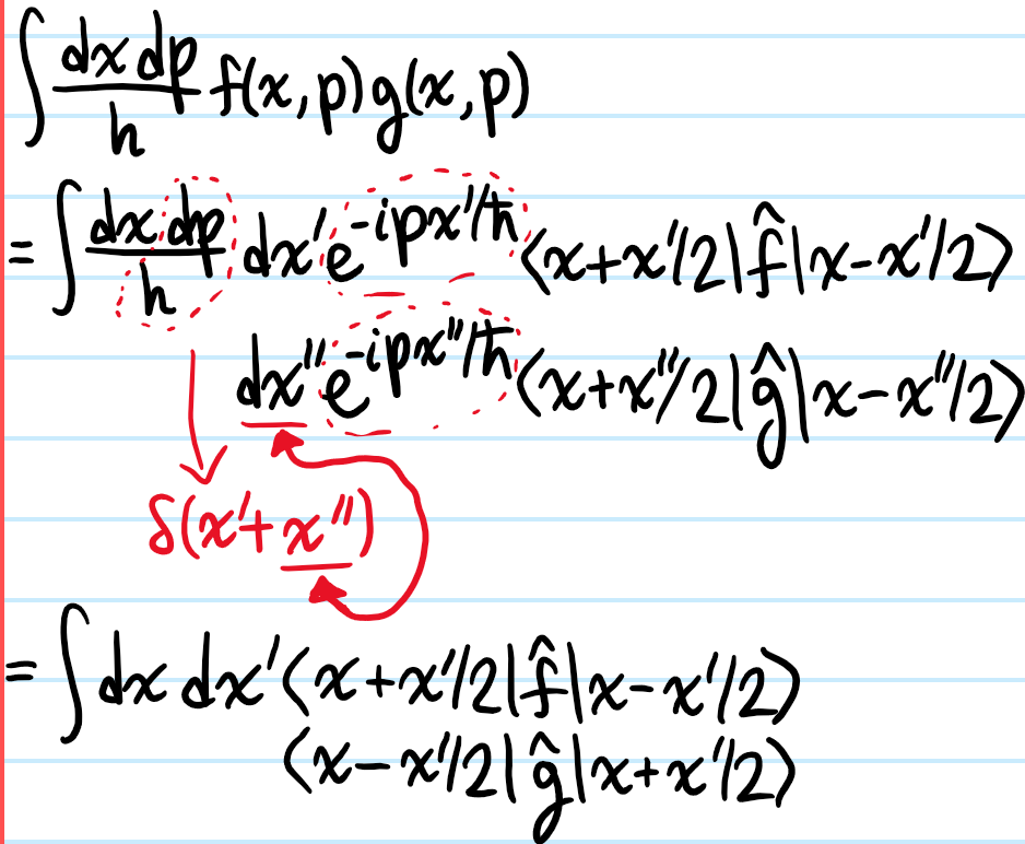
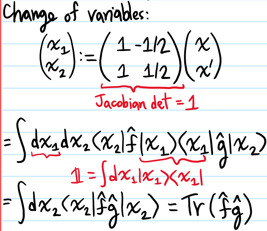
Problem: Show that, for any \(2\) arbitrary operators \(\hat f,\hat g\), the trace of their product may be written in terms of their Wigner transforms \(f(x,p),g(x,p)\) via the homomorphism:
Solution: It seems to be easier to go from RHS to LHS:
Problem: Define the Wigner quasiprobability distribution \(\rho(x,p)\).
Solution: Given a quantum mechanical system whose state space \(\mathcal H\) contains factors of \(L^2(\textbf R^3\to\textbf C)\) (i.e. spatial degrees of freedom), then the Wigner quasiprobability distribution is simply the Wigner transform of the system’s density operator \(\hat{\rho}\) divided by \(h\):
Problem: Hence, combining the previous results, show that the Wigner quasiprobability distribution \(\rho(x,p)\) has the following properties which warrant its name:
i) For any observable \(\hat H\), the expectation \(\langle \hat H\rangle\) in an arbitrary mixed ensemble with density operator \(\hat{\rho}\) is:
where \(\rho_{1,2}(x,p)\) are the respective Wigner quasiprobability distributions for \(\hat{\rho}_{1,2}:=|\psi_{1,2}\rangle\langle\psi_{1,2}|\).
v) For a normalized pure state, \(|\rho(x,p)|\leq 2/h\) is bounded on phase space \((x,p)\).
Solution:
i) This simply follows from \(\langle\hat H\rangle=\text{Tr}(\hat{\rho}\hat H)\) together with the earlier identity for the trace of a product (one should check that the Wigner transform of the identity operator is indeed \(1\)).
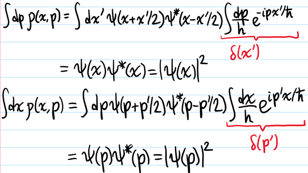
ii) Using the \(2\) different forms of \(\rho(x,p)\) derived earlier for a pure state (one w.r.t. position space wavefunctions, one w.r.t. momentum space wavefunctions) the derivation is very simple:
(more generally, if \(\hat\rho\) is impure, then one can still say \(\int dp\rho(x,p)=\langle x|\hat{\rho}|x\rangle\) and \(\int dx\rho(x,p)=\langle p|\hat{\rho}|p\rangle\)).
iii) This simply stems from the Hermiticity of any density operator \(\hat{\rho}^{\dagger}=\hat\rho\) which is logically equivalent to the reality of \(\rho(x,p)\in\textbf R\).
iv) This follows from the identity \(|\langle\psi_1|\psi_2\rangle|^2=\text{Tr}(\rho_1\rho_2)\). In particular, if \(\langle\psi_1|\psi_2\rangle=0\) are orthogonal, then this shows that, despite just showing that it’s real, the Wigner quasiprobability distribution clearly cannot always be positive, even for simple pure states; this is the key difference between it and the positive semi-definiteness of the density operator \(\hat{\rho}\). It is also the reason for the quasi prefix, reflecting the fact that although its marginals \(|\psi(x)|^2,|\psi(p)|^2\) do have legitimate probabilistic interpretations, funnily enough the joint distribution \(\rho(x,p)\) does not admit such an interpretation.
v) This follows simply from the Cauchy-Schwarz inequality after doing a substitution \(x’\mapsto x’/2\) in the Wigner integral transform.
Problem: Show that the Wigner quasiprobability \(\rho(x,p,t)\) flows through phase space with respect to a Hamiltonian \(H\) according to the Moyal equation:
\[\dot{\rho}+\{\rho,H\}_{\star}=0\]
where \(i\hbar\{\rho,H\}_{\star}=\rho\star H-H\star\rho\) is the Moyal bracket, and the star product \((f\star g)(x,p)\) of two functions \(f(x,p),g(x,p)\) on phase space is defined by the somewhat peculiar formula:
Problem: At a high level, what is the goal of classical hydrodynamics?
Solution: The program of classical hydrodynamics seeks to bridge the physics of a many-body system at different length scales. The idea is to start from microscopics (i.e. Newton’s laws) and derive mesoscopics (i.e. Boltzmann equation), and from there to derive macroscopics (i.e. Navier-Stokes equations). Of course, there is also a field of quantum hydrodynamics, but that’s for another day…
Problem: In light of the above, it is useful to start with Newton’s laws, but in their Hamiltonian formulation. In order to coarse grain from this microscopic description to a mesoscopic description, the natural way to achieve such a coarse graining is to construct (i.e. pull out of thin air!) a probability density function \(\rho(\textbf x_1,…,\textbf x_N,\textbf p_1,…,\textbf p_N,t)\) defined on the joint phase space \(\cong\textbf R^{6N}\) of the \(N\)-body system. Give a more precise interpretation to \(\rho\).
Solution: The precise interpretation is that \(\rho(\textbf x_1,…,\textbf x_N,\textbf p_1,…,\textbf p_N,t)d^3\textbf x_1…d^3\textbf x_Nd^3\textbf p_1…d^3\textbf p_N\) is the probability (purely due to classical ignorance) that the system of \(N\) (in general not necessarily identical) particles is, at some time \(t\), living within an infinitesimal volume \(d^3\textbf x_1…d^3\textbf x_Nd^3\textbf p_1…d^3\textbf p_N\) centered around the (micro)state \((\textbf x_1,…,\textbf x_N,\textbf p_1,…,\textbf p_N)\) in the joint phase space.
Problem: State the equation of motion obeyed by \(\rho\) (i.e. Liouville’s equation).
Solution: Remembering the intuition that \(\{\space\space,H\}\) implements an advective derivative on the joint phase space (the essence of Hamilton’s equations):
so probability flows incompressibly throughout phase space under \(H\).
Problem: From this joint probability density function \(\rho\), explain how to marginalize to obtain the single-particle probability density function \(\rho_1(\textbf x,\textbf p,t)\) for say “particle #\(1\)”.
Solution: Simply integrate away the \(6(N-1)\) degrees of freedom of the other \(N-1\) particles:
Thus, \(\rho_1(\textbf x,\textbf p,t)d^3\textbf x d^3\textbf p\) represents the probability (again due to classical ignorance) that “particle \(1\)” will, at some time \(t\), be found in the infinitesimal cell \(d^3\textbf xd^3\textbf p\) centered around the state \((\textbf x,\textbf p)\) in its (single-particle) phase space.
Problem: Henceforth suppose (as is often the case) that the \(N\) particles are identical. Explain what the best way is to exploit this additional assumption of indistinguishability.
Solution: Rather than working with \(\rho_1\), work with \(n_1:=N\rho_1\); this sort of like a classical analog of the quantum mechanical passage from first quantization (Slater permanent/determinants) to second quantization (occupation numbers) in many-body quantum mechanics of identical bosons/fermions.
Problem: Derive the analog of the Liouville equation for \(n_1(\textbf x,\textbf p,t)\) (a.k.a. the Boltzmann equation):
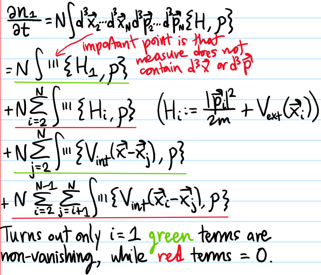
where \(n_2:=N(N-1)\int d^3\textbf x_3…d^3\textbf x_Nd^3\textbf p_3…d^3\textbf p_N\rho\). Specify the actual physics by assuming the Hamiltonian \(H\) has the generic dispersion:
where \(H_i:=\frac{|\textbf p_i|^2}{2m}+V_{\text{ext}}(\textbf x_i)\), and in general for \(i=1\) one writes \(\textbf x:=\textbf x_1\) and \(\textbf p:=\textbf p_1\).
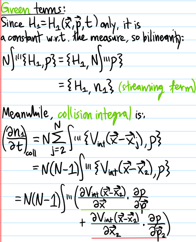
Solution: Using the Liouville equation for \(\rho\) as a springboard, the Boltzmann equation for \(n_1\) looks like:
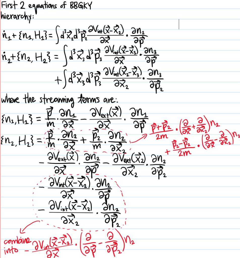
Problem: In writing the Boltzmann equation for \(\dot n_1\) above, it was natural to introduce the quantity \(n_2(\textbf x,\textbf x_2,\textbf p,\textbf p_2,t)\). If one were to repeat the above derivation, namely evaluate \(\dot n_2\) using Liouville’s equation for \(\dot{\rho}\) again, what result would one find?
Solution: One would get a result most naturally expressed in terms of a quantity \(n_3:=N(N-1)(N-2)\int d^3\textbf x_4…d^3\textbf x_Nd^3\textbf p_4…d^3\textbf p_N\rho\), and so forth. This ladder of \(N\) equations forms the BBGKY hierarchy:
and \(k\)-particle Hamiltonian \(H_k\) including both \(V_{\text{ext}}\) and interactions \(V_{\text{int}}\) among the first \(k\) particles but ignores interactions with the other \(N-k\) particles:
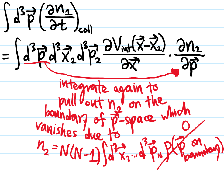
Problem: Define the real space number density \(n(\textbf x,t)\) in terms of \(n_1(\textbf x,\textbf p,t)\) and show that it’s not influenced by the collision integral.
Solution: One has \(n(\textbf x,t):=\int d^3\textbf p n_1(\textbf x,\textbf p,t)\). So:
but the \(d^3\textbf p\)-integral over the collision integral vanishes for the same kind of reasons as above:
Problem: What about for the momentum space number density \(n(\textbf p,t):=\int d^3\textbf x n_1(\textbf x,\textbf p,t)\)? What about for the real space momentum density \(\int d^3\textbf p\textbf pn_1\) or the real space kinetic energy density \(\int d^3\textbf p|\textbf p|^2n_1/2m\)?
Solution: In all these cases, the collision integral will contribute!
Problem: Show that a classical elastic \(2\)-body collision between equal-mass particles implies (though is not equivalent to) an \(O(3)\) isometry on their relative momentum.
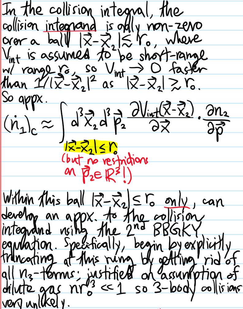
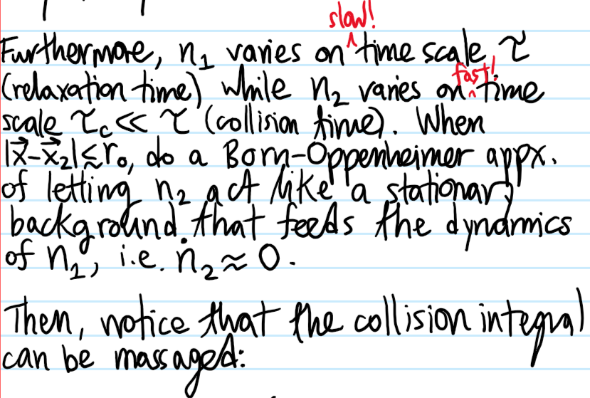
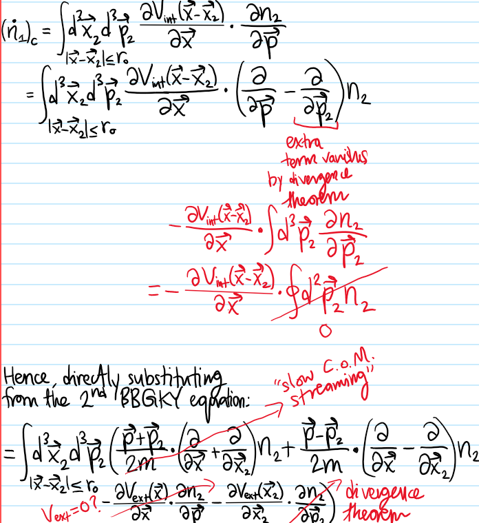
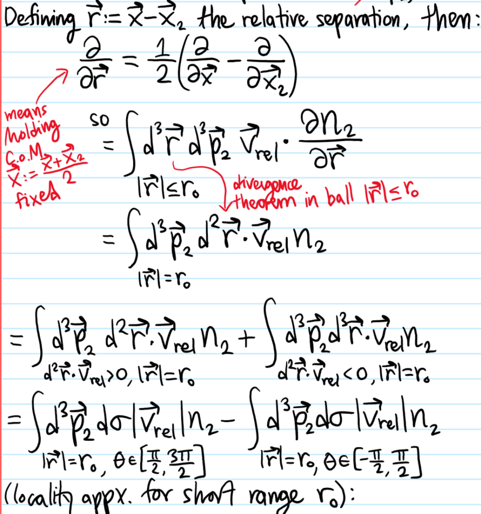
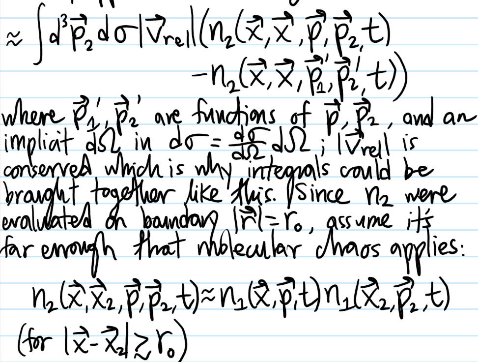
Problem: Strictly speaking, the above is actually a precursor to the actual Boltzmann equation. So then, how does the actual Boltzmann equation arise from the BBGKY hierarchy? Make sure to clearly identify all assumptions.
Solution:
One thus obtains the actual Boltzmann (integrodifferential!) equation for \(n_1\), which still asserts that:
where \(|\textbf v_{\text{rel}}|:=|\textbf p-\textbf p_2|/m=|\textbf p’_1-\textbf p’_2|/m\) is conserved, and in practice one should compute the differential cross-section \(d\sigma=\frac{d\sigma}{d\Omega}d\Omega\) from the interaction potential \(V_{\text{int}}\), and both post-collision momenta \(\textbf p’_1,\textbf p’_2\) are determined from \(\textbf p_1,\textbf p_2\) and \(d\Omega\) by elasticity.
On dimensional analysis grounds, the way to read the collision integral is as follows:
Problem: Elaborate more on the molecular chaos assumption and how it resolves Loschmidt’s paradox concerning the arrow of time \(t\).
Solution: The molecular chaos assumption essentially is the assertion that the pre-collision velocities are uncorrelated. The prefix “pre” is what breaks time reversal symmetry, despite the underlying Hamiltonian mechanics being time reversible.
but \(N=\int d^3\textbf xd^3\textbf pn_1\) is conserved so that \(\dot N=\int d^3\textbf xd^3\textbf p\dot n_1=0\). Then of course, one should invoke Boltzmann’s equation:
\[\int d^3\textbf x\frac{\partial n_1}{\partial\textbf x}\ln n_1=\oint d^2\textbf x n_1\ln n_1-\int d^3\textbf x\frac{\partial n_1}{\partial\textbf x}=\oint d^2\textbf x n_1(\ln n_1-1)=0\]
and similarly for the other term.
To complete the proof, one just has to show that the collision integral term is \(\leq 0\). This is slightly more delicate, requiring one to first symmetrize between the particles \(\textbf p\Leftrightarrow\textbf p_2\) to obtain:
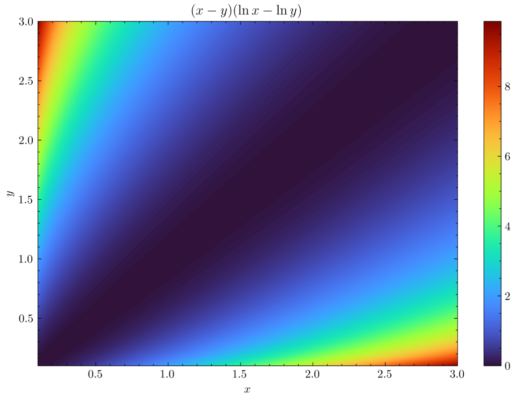
where \(x:=n_1(\textbf x,\textbf p’_1,t)n_1(\textbf x,\textbf p’_2,t)\) and \(y:=n_1(\textbf x,\textbf p,t)n_1(\textbf x,\textbf p_2,t)\). But the integrand is positive for all \(x,y>0\):
and “Boltzmann’s \(H\)-theorem” is proven.
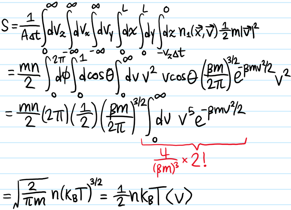
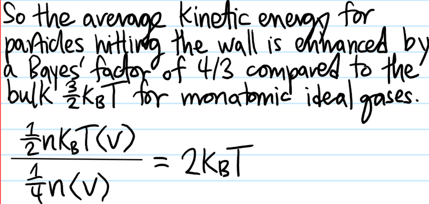
Problem: A given single-particle phase space number density distribution \(n_1(\textbf x,\textbf p,t)\) is said to be in detailed balance iff for all locations \(\textbf x\in\textbf R^3\) and momenta \(\textbf p,\textbf p_2,\textbf p’_1,\textbf p’_2\in\textbf R^3\) obeying \(\textbf p+\textbf p_2=\textbf p’_1+\textbf p’_2\) and \(|\textbf p|^2+|\textbf p_2|^2=|\textbf p’_1|^2+|\textbf p’_2|^2\) (i.e. elastic collisions), one has the identity:
\(n_1(\textbf x,\textbf p,t)=n(\beta/2\pi m)^{3/2}\exp(-\beta|\textbf p-m\textbf v|^2/2m)\) for some functions \(n(\textbf x,t),\textbf v(\textbf x,t),\beta(\textbf x,t)\) (this is also called the Maxwell-Boltzmann distribution or, more profoundly, local equilibrium, which reduces to the usual thermodynamic case of global equilibrium iff \(n, \textbf v, \beta\) are constant parameters rather than spatiotemporally varying).
Solution: First, assume that \(n_1\) is in detailed balance (aside: the adjective detailed in this context is roughly synonymous with the adjective pairwise; it emphasizes that the balance doesn’t just come from e.g. \(5\) people standing in a circle and each person passing an apple to the person on their left, but that if Alice gives Bob \(3\) apples then Bob will also give Alice \(3\) apples). Then clearly, this is just the \(y=x\) diagonal in the graph! Thus, \(\dot S=0\). #2 is also clearly seen to imply #1 thanks to Boltzmann’s \(H\)-theorem. It is also trivial to check #1 is equivalent to #3.
In addition, \(n_1\) is in detailed balance if and only if \(\ln n_1\) is a collisional invariant. Finally, #3 can be argued to imply #4 by the fact that, since \(\ln n_1\) is a collisional invariant, it must be a linear combination of other collisional invariants \(\ln n_1\in\text{span}_{\textbf R}(1,\textbf p,|\textbf p|^2\}\), so there exist parameters \(\mu, \beta, \textbf v\) such that:
where the “fugacity” \(z:=e^{\beta\mu}\) is fixed by the normalization \(n=\int d^3\textbf pn_1\), and results in the form stated. The converse is of course trivial to show.
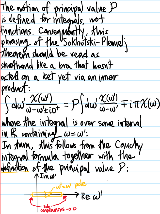
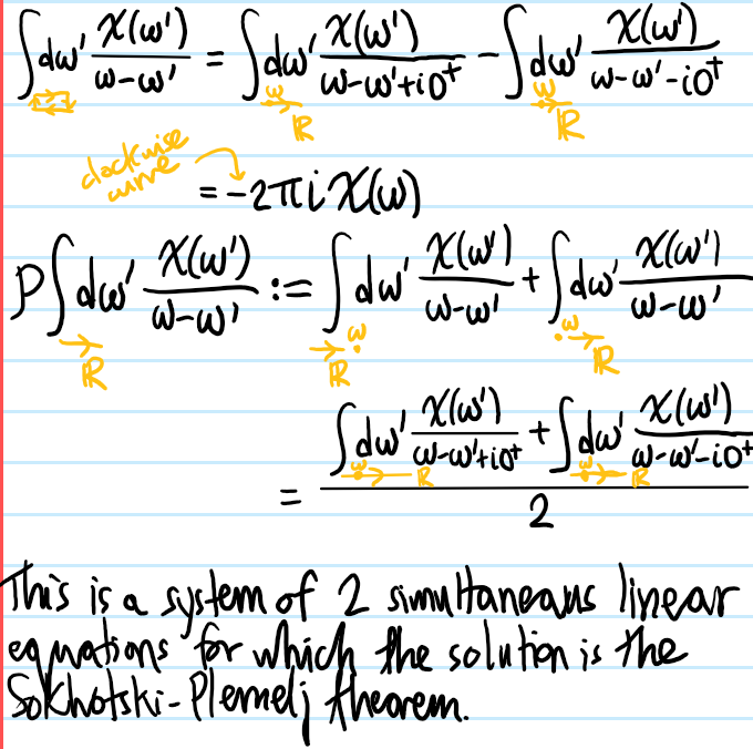
Solution: (in this solution, the function \(\chi(\omega)\) is assumed to be analytic on the integration interval in \(\textbf R\) to be able to apply the Cauchy integral formula):
Problem: Explain why any linear response function \(\chi\) should obey in the time domain \(\chi(t)=0\) for \(t<0\). Hence, what is the implication of this for \(\chi(\omega)\) in the frequency domain?
Solution: The fundamental definition of the linear response function \(\chi\) that gives it its name is that in the time domain \(\chi=\chi(t)\), the response \(x(t)\) should be proportional to the perturbation \(f(t)\) with \(\chi\) essentially acting as the proportionality constant according to the convolution:
(or equivalently the local behavior \(x(\omega)=\chi(\omega)f(\omega)\) in Fourier space). But if the “force” \(f(t’)\) is applied at time \(t’\), on causality grounds this can only affect the response \(x(t)\) at times \(t\geq t’\). In other words, it should be possible to change the limits on the integral from \(\int_{-\infty}^{\infty}dt’\) to \(\int_{-\infty}^tdt’\) without affecting the result. This therefore requires \(\chi(t-t’)=0\) for \(t<t’\), or more simply \(\chi(t)=0\) for \(t<0\). In light of this, \(\chi\) is also called a causal/retarded Green’s function.
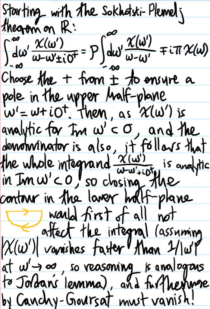
For \(t<0\), Jordan’s lemma asserts that one should close the contour in the lower half-plane \(\Im\omega<0\). But the fact that \(\chi(t)=0\) for \(t<0\) suggests that the sum of all residues of \(\chi(\omega)\) in the lower half-plane \(\Im\omega<0\) should be “traceless”. A sufficient condition for this is if \(\chi(\omega)\) is analytic in the lower half-plane \(\Im\omega<0\), and henceforth this will be assumed.
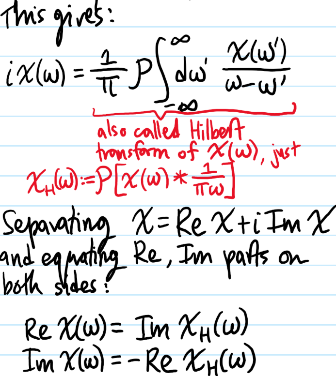
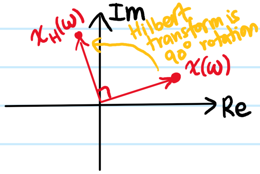
Problem: Qualitatively, what do the Kramers-Kronig relations assert? What about quantitatively?
Solution: Qualitatively, for a linear response function like \(\chi(\omega)\) which is analytic in the lower half-plane \(\Im\omega<0\), knowing its reactive part \(\Re\chi(\omega)\) is equivalent to knowing its absorptive/dissipative spectrum \(\Im\chi(\omega)\) which in turn is equivalent to knowing \(\chi(\omega)\) itself.
Quantitatively, the bridges \(\Leftrightarrow\) are provided by the Kramers-Kronig relations:
Note: sometimes the discussion of Kramers-Kronig relations are phrased in terms of \(\chi(\omega)\) being analytic in the upper half-plane. This stems from an unconventional definition of the Fourier transform \(\chi(t)=\int_{-\infty}^{\infty}\frac{d\omega}{2\pi}e^{-i\omega t}\chi(\omega)\) rather than the more conventional definition \(\chi(t)=\int_{-\infty}^{\infty}\frac{d\omega}{2\pi}e^{i\omega t}\chi(\omega)\) used above. Consequently, the minus signs in the Kramers-Kronig relations may also appear flipped around.
Problem: If the response \(x(t)\) and the driving force \(f(t)\) are both real-valued, what are the implications of this for \(\Re\chi(\omega)\) and \(\Im\chi(\omega)\)?
Solution: Then \(\chi(t)\in\textbf R\) must also be real-valued, so \(\chi(\omega)\) is Hermitian:
\[\chi^{\dagger}(\omega)=\chi(-\omega)\]
Consequently, the reactive response \(\Re\chi(-\omega)=\Re\chi(\omega)\) is even while the absorptive/dissipative response \(\Im\chi(-\omega)=-\Im\chi(\omega)\) is odd.
Problem: State the thermodynamic sum rule.
Solution: The sum rule asserts that if one knows how much a system absorbs/dissipates at all frequencies \(\omega\in\textbf R\), then one can deduce the system’s DC linear response \(\chi(\omega=0)\), called its susceptibility (of course the Kramers-Kronig relations actually show that knowing \(\Im\chi(\omega)\) allows complete reconstruction of \(\chi(\omega)\) at all frequencies \(\omega\in\textbf R\), not just \(\omega=0\)).
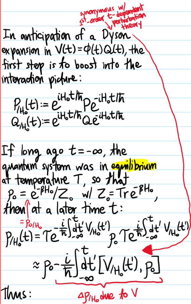
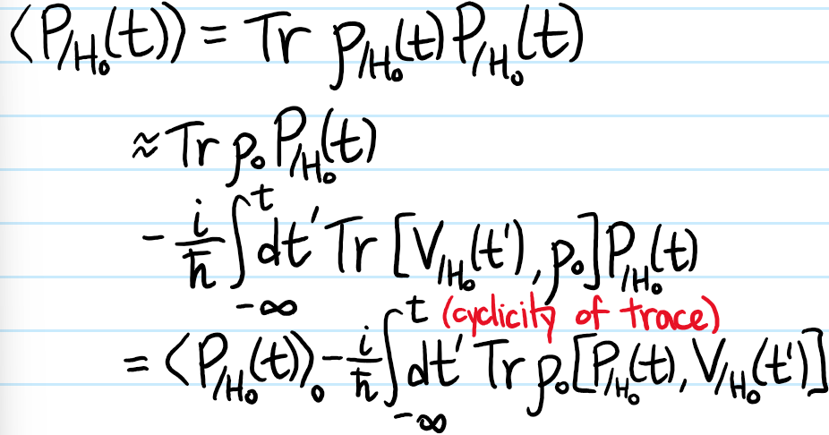
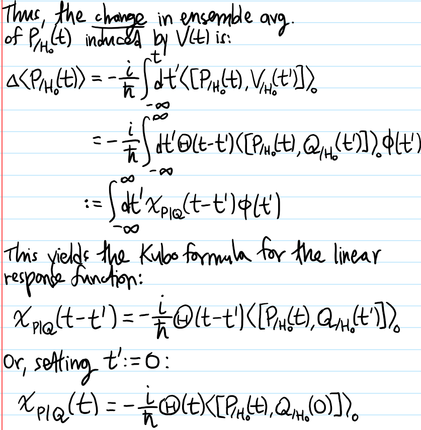
Problem: Given a \(t\)-dependent Legendre perturbation of the form \(V(t)=\phi(t)Q\) where \(Q\) is a (possibly also \(t\)-dependent) operator and \(\phi(t)\) is scalar-valued, define the linear response function \(\chi_{P|Q}(t)\) of another operator \(P\) due to \(Q\) and show that within the framework of linear response theory it is given by Kubo’s formula:
Problem: Distinguish between a supervised dataset and unsupervised dataset.
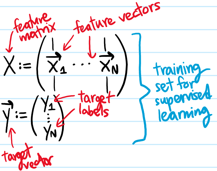
Solution: Supervised data is of the form \(\{(\textbf x_1,y_1),…,(\textbf x_N,y_N)\}\). Unsupervised data consists of stripping away the target labels \(y_1,…,y_N\), leaving behind just the feature vectors \(\{\textbf x_1,…,\textbf x_N\}\).
Problem: \(k\)-means clustering is an unsupervised learning algorithm (not to be confused with \(k\)-nearest neighbors which is a supervised learning algorithm) which arguably is easier to explain in words than with math. Hence, explain it in words.
Solution: Start with an unsupervised data set \(\textbf x_1,…,\textbf x_N\in\textbf R^n\) of feature vectors, and initialize some number \(k\leq N\) of “cluster centroids” \(\boldsymbol{\mu}_1,…,\boldsymbol{\mu}_k\in\textbf R^n\). Then, repeat the following \(2\)-step algorithm:
Partition the unsupervised data set of feature vectors \(\{\textbf x_1,…,\textbf x_N\}\) into \(L^2\)-Voronoi clusters with respect to the cluster centroids \(\boldsymbol{\mu}_1,…,\boldsymbol{\mu}_k\).
Update the locations of each cluster centroid \(\boldsymbol{\mu}_1,…,\boldsymbol{\mu}_k\) to the mean of the feature vectors associated to its \(L^2\)-Voronoi cluster.
Problem: What is the so-called distortion cost function \(C\) that \(k\)-means clustering seeks to minimize? Intuitively, why does it work?
Solution: There are \(2\) distinct theorems one can prove, which justify respectively the \(2\) steps of the \(k\)-means clustering algorithm described above. Informally, in the space \(\textbf R^n\) one has \(N+k\) characters, namely the \(N\) feature vectors \(\textbf x_1,…,\textbf x_N\) and the \(k\) cluster centroids \(\boldsymbol{\mu}_1,…,\boldsymbol{\mu}_k\).
Theorem #\(1\): Fix both the locations of the \(N\) “households” \(\textbf x_1,…,\textbf x_N\) and the \(k\) “wells” \(\boldsymbol{\mu}_1,…,\boldsymbol{\mu}_k\). Define the distortion cost functional \(C[\boldsymbol{\mu}^*]\) for a choice of household-to-well allocation \(\boldsymbol{\mu}^*:\{\textbf x_1,…,\textbf x_N\}\to\{\boldsymbol{\mu}_1,…,\boldsymbol{\mu}_k\}\) by the formula:
Theorem #\(2\):Fix only the locations of the \(N\) “households” \(\textbf x_1,…,\textbf x_N\), and fix the allocation \(\boldsymbol{\mu}^*\) from Theorem #\(1\). Define the distortion cost function:
Then, if a contractor were allowed to come and relocate the \(k\) “wells” \(\boldsymbol{\mu}_1,…,\boldsymbol{\mu}_k\mapsto\boldsymbol{\mu}’_1,…,\boldsymbol{\mu}’_k\), then \(\partial C/\partial(\boldsymbol{\mu}’_1,…,\boldsymbol{\mu}’_k)=\textbf 0\) for:
Problem: How should the cluster centroids \(\boldsymbol{\mu}_1,…,\boldsymbol{\mu}_k\) be initialized?
Solution: Do \(50\to 1000\) random initializations of the \(k\) means on the feature vectors themselves, and run the algorithm to convergence. Each time, one will get some configuration of clusters with an associated minimized distortion cost \(C_*\). Then, just take the cluster with the lowest \(C_*\).
Problem: How should the number of clusters \(k\in\textbf Z^+\) be selected?
Solution: This is more of an art than a science (one heuristic is to plot the minimized distortion cost function \(C_*\) against \(k\) and look for the “elbow”, alternatively one can just vary \(k\) and, for each clustering that results, empirically see which one is best for whatever downstream application one has in mind.
Problem: Describe how anomaly detection works.
Solution: Given a bunch of unlabelled feature vectors \(\textbf x_1,…,\textbf x_N\in\textbf R^n\) each with \(n\) scalar features, the idea is to assume that they are i.i.d. draws from an underlying normal random vector \(\textbf x\) with mean \(\boldsymbol{\mu}\) and covariance matrix \(\sigma^2\), i.e.
Thus, for a given probability density threshold \(\varepsilon>0\), the isosurface \(\rho(\textbf x)=\varepsilon\) in \(\textbf R^d\) defines an ellipsoid centered at \(\boldsymbol{\mu}\). If a draw of \(\textbf x\) lies outside of this ellipsoid so that \(\rho(\textbf x)<\varepsilon\), then one would classify or “detect” this \(\textbf x\) as an “anomaly”.
Note that typically, if the features are uncorrelated, then \(\sigma\) may be taken diagonal, which is equivalent to asserting that all \(n\) scalar features are also normal random variables. If this is not initially the case, one can often artificially enforce it by performing some suitable transformation of the scalar features to make them “more Gaussian”. As usual, the techniques of error analysis and feature engineering apply here.
Problem: How should the probability density threshold \(\varepsilon\) be chosen in anomaly detection?
Solution: By definition of an “anomaly”, it is typically the case that the vast majorities of draws from \(\textbf x\) will be “normal”, i.e. not anomalous. Therefore, any given training set \(\textbf x_1,…,\textbf x_N\) will likely be highly skewed. For this reason, it is often a good idea to maximize the \(F_1\)-score on a cross-validation set as a function of \(\varepsilon\), by trial-and-error with various values of \(\varepsilon\).
Problem: The objective of anomaly detection is essentially identical to that of supervised binary classification; anomalous examples might be labelled \(1\) whereas normal examples are labelled \(0\). So when should one use anomaly detection vs. supervised binary classification?
Solution: One key idea lies again in the definition of the word “anomaly” as suggesting a deviation from the norm which is furthermore rare. Therefore, the idea is as follows: suppose one initially were planning to do supervised binary classification. Then, because this is supervised learning, in addition to the feature vectors, each training example would also need to be accompanied by its target label \(y\in\{0,1\}\). If one goes ahead and manually labels each feature vector \(\textbf x\) by its corresponding \(y\), and one finds that the number of \(y=0\) labels vastly outnumbers the \(y=1\) labels (or vice versa), then this suggests that it may be more prudent to interpret this as an anomaly detection problem rather than supervised binary classification.
Another useful cue lies in asking the question “how many ways are there to be anomalous?”. If there are many ways by which an example could be anomalous, and one isn’t interested in exactly which way but only to have a large “wastebasket” to collect all anomalous examples…well then as one may anticipate, anomaly detection is the way to go.
Problem: Explain what the objective of collaborative filtering is.
Solution: The objective is loosely similar to filling out a Sudoku grid, or in a pure math context, trying to predict missing entries in a matrix. The context in which collaborative filtering is typically discussed centers around recommender systems in the sense that one might have a matrix \(Y_{mu}\) with \(1\leq m\leq N_m\) representing \(N_m\) movies and \(1\leq u\leq N_u\) representing \(N_u\) users, and some entries of this \(N_m\times N_u\) matrix \(Y_{mu}\) are filled with movie ratings (e.g. from \(0\to 5\)) given by certain users, but since not all users have rated all movies yet (because they haven’t watched them), the goal is to predict what they would rate the movie, hence whether they would like it or not, hence whether it should be recommended to them. Simply put, “filtering” and “recommending” in this context are synonymous, so actually I personally think a better name would have been “collaborative recommending”.
Problem: Write down the collaborative filtering cost function \(C(\textbf w_1,…,\textbf w_{N_u},b_1,…,b_{N_u},\textbf x_1,…,\textbf x_{N_m}|Y, \lambda)\)
Solution: Essentially, one just uses a (bi)linear regression model \(\hat Y_{mu}=\textbf w_u\cdot\textbf x_m+b_u\):
But note that in the double series, since \(Y_{mu}\) is only defined for movies \(m\) where user \(u\) has actually given a rating, the sum should only be taken over matrix elements for which \(Y_{mu}\) exists.
As an aside, if instead \(Y_{mu}\in\{0,1\}\) are restricted to binary ratings, then a binary cross-entropy loss function would be more appropriate:
Finally, an important point often glossed over is that, in order to be able to compute the dot product \(\textbf w_u\cdot\textbf x_m\), both the user weight vectors \(\textbf w_u\) and the movie feature vectors \(\textbf x_m\) need to be equidimensional, but the exact value of this dimension is another degree of freedom that one can play around with.
Problem: How is content-based filtering similar to and distinct from collaborative filtering? What weaknesses of collaborative filtering does content-based filtering address?
Solution: Both content-based filtering and collaborative filtering seek to recommend items (e.g. movies) to users; in other words, both are still recommender systems. They differ in what information they use to make their recommendations.
Whereas collaborative filtering uses other users’ ratings to predict unknown ratings, without taking into account any features about the user or movies, content-based filtering assumes that one has access to this kind of additional information and so is able to make more tailored recommendations even to e.g. a first-time user who has never rated any movies before (thus, content-based filtering solves the cold-start problem of collaborative filtering).
The idea is that each user \(1\leq u\leq N_u\) has an associated feature vector \(\textbf w_u\) (previously thought of as an abstract “weight vector”) and similarly each movie \(1\leq m\leq N_m\) also has an associated feature vector \(\textbf x_m\). The idea of content-based filtering is to train \(2\) neural networks, one which maps user features \(\textbf w_u\mapsto\hat{\textbf u}_u\), and another which maps movie features \(\textbf x_m\mapsto\hat{\textbf v}_m\), where \(\textbf w_u\) and \(\textbf x_m\) need not have the same dimension but \(\hat{\textbf u}_u\) and \(\hat{\textbf v}_m\) must be equidimensional unit vectors; this is because, ultimately, the prediction model will be a zero-bias form of linear regression, i.e. the cosine similarity
Solution: Formally, a Markov decision process is a \(4\)-tuple \((S,A,P,R)\), where \(S\) is called the state space, \(A\) is called the action space (equipped with a group action on \(S\)?), \(P(\textbf s’|\textbf s,a)\) is a conditional probability function for being in a state \(\textbf s’\in S\) given one is in state \(\textbf s\in S\) and applies action \(a\in A\), and \(R:S\to\textbf R\) is a reward function specifying the reward \(R(\textbf s)\) of each state \(\textbf s\in S\).
Informally, the important point about an MDP is that it is memoryless, like a \(1^{\text{st}}\)-order ODE in \(t\) (e.g. Schrodinger’s equation), it given an initial condition at \(t=0\), then the subsequent time evolution is uniquely specified, it doesn’t matter whatever was happened for \(t<0\).
Problem: Define the return functional \(R[\textbf s(t)]\) of a path \(\textbf s(t)\) in state space \(S\).
Although in practice, because the path \(\textbf s(t)\) is stroboscopic due to discrete \(t\), this path integral always just reduces to a discrete series. In addition, time \(t\) starts from \(t=0\) until one reaches some terminal state, and the discount factor \(\gamma\in [0,1)\) is typically \(\approx 0.99\) or something like that, giving rise to delayed rewards.
Problem: What does it mean to say that \(\pi\) is a policy for a particular Markov decision process?
Solution: It means that \(\pi:S\to A\) is a function which, given the current state \(\textbf s\in S\) of the MDP, says which action \(\pi(\textbf s)\in A\) to apply (which would result in ending up at some other state \(\textbf s’\in S\) with probability \(P(\textbf s’|\textbf s,a)\)).
Problem: What is the goal of reinforcement learning?
Solution: To find the optimal policy \(\pi^*\) maximizing the expected return \(\langle R[\textbf s(t)]\rangle\), where the trajectory \(\textbf s(t)\) is determined by the choice of policy \(\pi^*\).
Problem: Define the state-action value function \(Q:S\times A\to\textbf R\), and state the \(2\) key theorems about it that motivate why it’s a useful construction.
i.e. the return from starting in state \(s\), then doing action \(a\), and then acting optimally from there onward. The \(2\) key properties of the \(Q\)-function are:
Theorem #\(1\): The expected max return from any state \(\textbf s\in S\) is \(\langle \text{max}_{a\in A}Q(\textbf s,a)\rangle\).
which follows trivially from the definition of the \(Q\)-function, more precisely from the \(\pi^*\) part of that definition; thus in a way the Bellman equation is a bit like a recurrence relation where the reward is what one gets right away \(r(\textbf s)\) plus the delayed rewards that one gets in the future.
Problem: Give a reasonable example of a state vector \(\textbf s\) for an autonomous truck driving application, and for an autonomous helicopter.
Solution: In both of these cases, one is working with a continuous-state MDP, since the state space \(S\) is uncountably infinite. For a truck, one might have:
Problem: Tying together all the previous problems, describe the optimized version of deep reinforcement learning using a deep-\(Q\)-network (DQN).
Solution: The idea is to use a neural network which takes a state vector \(\textbf s\) in its input layer and, in the output layer, seeks to estimate the \(Q\)-function evaluated on \(\textbf s\), for all possible actions \(a\in A\), i.e. estimate a vector of length \(\#A\) whose components are \(Q(\textbf s,a)\) for \(a\in A\).
Then, as with any supervised regression problem, one needs to first train the DQN on some labelled training examples (in mini-batches for speed and with soft updates for reliability). This is where the Bellman equation comes in. Using say a physics engine simulator (or in real life?), one can initialize the system in different states \(\textbf s\in S\), perform all possible actions \(a\in A\), and simply observe what state \(\textbf s’\in S\) the system is “scattered” into afterwards. Then, assuming one has pre-specified a reward function \(r\) so that \(r(\textbf s)\) is known, and the discount factor \(\gamma\) is also pre-set, and by randomly initializing the weights and biases in the neural network, one can get an (initially rather poor) estimate of \(Q(\textbf s’,a’)\) for all actions \(a’\in A\), thereby allowing one to get \(\text{max}_{a’}Q(\textbf s’,a’)\), and hence estimate \(Q(\textbf s,a)\) from the Bellman equation (i.e. as a target label).
Then, just minimize the usual MSE cost function with gradient descent.
One more important tip during training is that, rather than always follow \(\pi^*\), it is a good idea to use an \(\varepsilon\)-greedy policy (a misnomer; a better name would be the \((1-\varepsilon)\)-greedy policy):
\[\pi_{\varepsilon}(\textbf s):= \begin{cases} \text{argmax}_{a\in A} Q(s,a), & \text{with probability } 1-\varepsilon \\ \text{random } a\in A, & \text{with probability } \varepsilon \end{cases}\]
where the greedy action is also called exploitation while the random action is called exploration. When just beginning training, take \(\varepsilon\approx 1\) but decrease it gradually towards \(\varepsilon\to 0\).
Problem: In a multilayer perceptron(MLP), how are layers conventionally counted?
Solution: The input layer \(\textbf x\equiv\textbf a^{(0)}\) is also called “layer \(0\)”. However, if someone says that an MLP has e.g. \(7\) layers, what this means is that in fact it has \(6\) hidden layers \(\textbf a^{(1)},\textbf a^{(2)},…,\textbf a^{(6)}\), together with the output layer \(\textbf a^{(7)}\). In other words, the input layer \(\textbf a^{(0)}\) is not counted by convention.
Problem: Write down the formula for the activation \(a^{(\ell)}_n\) of the \(n^{\text{th}}\) neuron in the \(\ell^{\text{th}}\) layer of a multilayer perceptron (MLP)artificial neural network.
Solution: Using a sigmoid activation function, the activation of the \(n^{\text{th}}\) neuron in the \(\ell^{\text{th}}\) layer is:
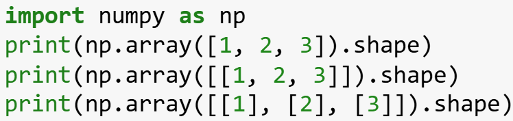
Problem: What is the output from the following Python code?
Solution: The first NumPy array has shape \((3,)\). The second NumPy array has shape \((1,3)\). The third NumPy array has shape \((3,1)\). While this may seem like a trivial distinction, in fact it’s very important when it comes to using the TensorFlow library, which only accepts matrices of the latter \(2\) kind.
Problem: What type of activation function is most often used for the hidden layers of an MLP? What about for the output layer?
Solution: The most common activation function for the hidden layers is the ReLU (rectified linear unit), defined as \(a_{\text{ReLU}}(x):=\text{max}(0,x)\) whereas the activation function used for the output layer depends on the range of target labels \(y\) (i.e. if it’s about binary classification \(y\in\{0,1\}\) then a sigmoid activation would be useful, if it’s \(y\in[0,\infty)\) then another ReLU would be useful, and if it’s \(y\in\textbf R\) then a linear activation function, would be useful; there are also other more exotic activation functions possible).
There are \(2\) reasons for using ReLU (rather than the historical sigmoid functions). The first (less important) reason is that ReLU is clearly a bit faster to compute than a sigmoid. The second (more important) reason is that experimentally one finds \(\partial/\partial(W,\textbf b)\)-descent is faster with ReLU than with sigmoids (intuitively this is due to the presence of more “flat” sections on the graph of the sigmoid than the ReLU).
Naturally one might also ask “why not just linear activations all the way through”? The reason is because this would just reduce to linear regression (i.e. the neural network wouldn’t buy one anything new). Similarly, changing the activation of the output layer to a sigmoid while keeping the hidden layers as linear activations just reduces to logistic classification.
Problem: Import the subset of training examples in the MNIST database whose target value is either \(y=0\) or \(y=1\), and train a multilayer perceptron with \(3\) hidden layers \((N_1,N_2,N_3)=(25,15,1)\) to do logistic binary classification on this subset (and evaluate the accuracy, and for fun have a look at the misclassified images).
Solution:
MNIST_test.html
In [1]:
importtensorflowastf# Load the MNIST dataset(x_train,y_train),(x_test,y_test)=tf.keras.datasets.mnist.load_data()print(x_train.shape)# (60000, 28, 28)print(y_train.shape)# (60000,)
# Get only the subset of training examples in the MNIST database whose target label is either 0 or 1subset_Boolean=(y_train<2)x_train_01_only=x_train[subset_Boolean,:,:]x_train_01_only.shape#(12665, 28, 28)y_train_01_only=y_train[subset_Boolean]y_train_01_only.shape#(12665,)# Reshape to (60000, 28*28) to be compatible with TensorFlow MLP.fit laterx_train_01_only_reshaped=x_train_01_only.reshape(x_train_01_only.shape[0],-1)
<keras.src.callbacks.history.History at 0x25370d10350>
In [6]:
# Some testing examples (TESTING = NOT TRAINING!)plt.figure(figsize=(15,15))forninnp.arange(5):plt.subplot(2,5,n+1)plt.imshow(x_test[n,:,:],cmap='gray')plt.title(f"Target Label: {y_test[n]}")
In [7]:
subset_Boolean=(y_test<2)x_test_01_only=x_test[subset_Boolean,:,:]x_test_01_only.shape#(2115, 28, 28)y_test_01_only=y_test[subset_Boolean]y_test_01_only.shape#(2115,)# Reshape to (60000, 28*28) to be compatible with TensorFlow MLP.fit laterx_test_01_only_reshaped=x_test_01_only.reshape(x_test_01_only.shape[0],-1)
probs=MLP.predict(x_test_01_only_reshaped)# shape (N, 1)y_hat=(probs>=0.5).astype(int).reshape(-1)# shape (N,), can also use .ravel()accuracy=(y_hat==y_test_01_only).mean()print(f"MLP Binary Classification Accuracy: {accuracy:.4f}")
# Which one was misclassified?deviation_Booleans=(y_hat!=y_test_01_only)x_test_01_only_deviations=x_test_01_only[deviation_Booleans]y_test_01_only_deviations=y_test_01_only[deviation_Booleans]len(x_test_01_only_deviations)#4plt.figure(figsize=(20,15))fori,test_xinenumerate(x_test_01_only_deviations):plt.subplot(2,5,i+1)plt.imshow(test_x,cmap='gray')plt.title(f"Target Label: {y_test_01_only_deviations[i]}, MLP Prediction: {y_hat[deviation_Booleans][i]}")
Problem: Write down the activations of a softmax output layer with \(N_{\text{out}}\) neurons to be used for multiclass classification with \(N_{\text{out}}\) classes.
Solution: For \(1\leq n\leq N_{\text{out}}\), define the conventional variables \(z_n:=\textbf w_n\cdot\textbf x+b_n\), where \(\textbf w_n,b_n\) are the weights and bias of the \(n^{\text{th}}\) neuron in that \(N_{\text{out}}\)-neuron output layer, and \(\textbf x\) here represents the activation vector of the previous (hidden) layer of neurons. Then the softmax activation of the \(n^{\text{th}}\) neuron in that output layer is given by:
which is the usual definition of informationcontent.
Problem: Explain why softmax classification is a generalization of logistic classification.
Problem: Suppose one is deciding between several possible neural network architectures. One has a bunch of data \(\mathcal D:=\{(\textbf x_i,y_i)\}\) on one’s hands. What is a quantitative way to perform model selection in this case (i.e. decide which neural network architecture to use)?
Solution: First, randomly partition the data set \(\mathcal D\) into \(3\) disjoint subsets \(\mathcal D=\mathcal D_{\text{tr}}\cup\mathcal D_{\text{cv}}\cup\mathcal D_{\text{te}}\), viz. a training subset \(\mathcal D_{\text{tr}}\), a cross-validation subset \(\mathcal D_{\text{cv}}\), and a testing subset \(\mathcal D_{\text{te}}\); note as a rule of thumb the size of these subsets in relation to the original data set should be around \(\#\mathcal D_{\text{tr}}/\#\mathcal D\approx 60\%\) and \(\#\mathcal D_{\text{cv}}/\#\mathcal D\approx \#\mathcal D_{\text{te}}/\#\mathcal D\approx 20\%\). Then, each of these \(3\) subsets plays its respective role for each of the \(3\) steps:
For each neural network architecture, minimize \(C_{\mathcal D_{\text{tr}}}(\{\textbf w_n^{(\ell)}\},\{b_n^{(\ell)}\}|\lambda=0)\), thereby obtaining a set of optimal weights \(\{\textbf w_n^{(\ell)*}\}\) and optimal biases \(\{b_n^{(\ell)*}\}\) for the neurons in that particular neural network architecture.
For each neural network architecture, using its optimal \(\{\textbf w_n^{(\ell)}\},\{b_n^{(\ell)}\}\) from step \(1\), evaluate \(C_{\mathcal D_{\text{cv}}}(\{\textbf w_n^{(\ell)*}\},\{b_n^{(\ell)*}\}|\lambda=0)\). The neural network one should choose is then the one for which this cross-validation error is the minimum.
(Optional) An unbiased estimator for that neural network’s generalization error is then given by \(C_{\mathcal D_{\text{te}}}(\{\textbf w_n^{(\ell)*}\},\{b_n^{(\ell)*}\}|\lambda=0)\). This is unbiased because neither the particular neural network architecture nor its weights and biases were determined from \(\mathcal D_{\text{te}}\).
Problem: Explain the difference between a model’s representational capacity and its effective capacity.
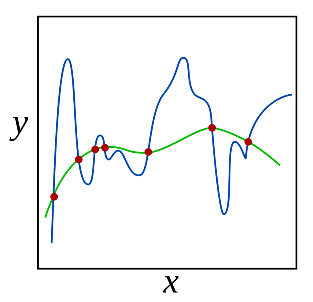
Solution: The representational capacity of a model is essentially asking about how many possible functions can be reached by the ansatz. For example, a quadratic model \(\hat y(x|w_1,w_2,b)=w_1x^2+w_2x+b\) clearly has greater representational capacity than the linear model \(\hat y(x|w,b)=wx+b\) because the function space spanned by the latter is a subset of the function space spanned by the former. In practice, the true representational capacity of a model may be difficult to exploit due to the nonconvex optimization landscape. Taking this limitation into account yields the concept of an effective capacity which is always less than or equal to the model’s representational capacity.
Problem: For a binary classifier, explain how the Vapnik-Chervonenkis (VC) dimension \(\dim_{\text{VC}}\) provides an integer proxy for its representational capacity.
Solution: One can first define a slightly more general concept of VC dimension \(\dim_{\text{VC}}\) for any arbitrary collection \(\mathcal C\) of sets.
A collection of sets \(\mathcal C\) is said to shatter a set \(X\) iff every subset of \(X\) can be “carved out” by taking \(X\) and intersecting it with some set in \(\mathcal C\); this is equivalent to saying that the power set \(2^X=\mathcal C\cap X\) where \(\mathcal C\cap X\) is defined in the obvious manner.
The VC dimension \(\dim_{\text{VC}}\) of the collection \(\mathcal C\) of sets is then defined to the cardinality of the largest set \(X\) which can be shattered by \(\mathcal C\).
The way this applies to a binary classifier is that because a binary classifier works by taking feature space (e.g. \(\mathbf R^n\)) and dividing it up into \(2\) disjoint regions (such that features on one side of the boundary are classified \(0\) while features on the other side are classified \(1\)), \(\mathcal C\) is taken to be the collection of all such regions that can be classified as e.g. \(1\) for instance. Then \(X\) is simply the collection of feature vectors in that feature space (e.g. \(\mathbf R^n\)).
For example, the classic XOR counterexample provides an intuition for why the VC dimension of any linear binary classifier in the plane \(\mathbf R^2\) is \(\dim_{\text{VC}}=3\) (and in fact more generally the VC dimension of a linear binary classifier is \(\dim_{\text{VC}}=n+1\) in \(\mathbf R^n\)).
Problem: Show that the mean-squared error (MSE) admits a decomposition into \(3\) non-negative terms of the form:
and give expressions for all \(4\) terms in this equation. Using this identity, explain the bias-variance tradeoff.
Solution: The mean squared error of a point estimator \(\hat y=\hat y(x)\) for an underlying random variable \(y=y(x)\) is in this case a proxy for generalization error:
The Bayes error is an irreducible error associated with the random-variable nature of \(y\) itself rather than the model \(\hat y\) (e.g. \(2\) houses with the exact same features selling for different prices in a regression model, or \(2\) emails with identical features but one is spam and another isn’t in a classification model):
\[\text{Bayes error}=\sigma^2_y\]
(aside: the reason this is called a Bayes error is that \(y\) is being treated as a random variable rather than how a frequentist would view \(y\) as a fixed parameter…clearly if \(y\) were simply fixed then there would be no variance \(\sigma^2_y=0\) and hence no Bayes error).
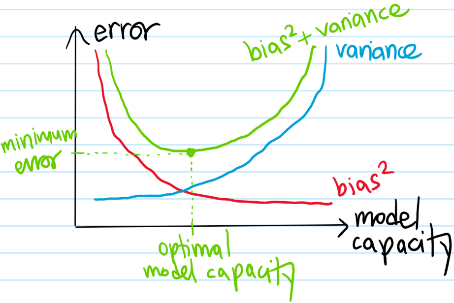
Since the Bayes error is generally not in one’s control, it follows that the best one can in principle hope for is \(\text{MSE}=\text{Bayes error}\), so this begs the question of how one can minimize the sum of \(\text{Bias}^2+\text{Variance}\)? Here, the dilemma of the bias-variance tradeoff is observed, namely \(\text{Bias}^2\) tends to be an decreasing function of the model’s effective capacity whereas \(\text{Variance}\) tends to be an increasing function of the effective capacity of \(\hat y\):
The challenge is thus to find that sweet spot in model capacity (also called model complexity/flexibility, etc.) that minimizes the sum \(\text{Bias}^2+\text{Variance}\) of these \(2\) errors as much as possible, since that’s all one has control over. If the model capacity is less than this optimal capacity, then one would be in a high-bias, low-variance regime of underfitting. By contrast, if the model capacity exceeds the optimal model capacity, then this low-bias, high-variance regime would be at risk of overfitting.
Practically, one can use as a proxy for diagnosis:
where \(C_0\) is some notion of “baseline cost” (e.g. human performance).
Problem: The previous problem explained how to diagnose high bias or high variance in a neural network model. Once they have been diagnosed, what’s the cure?
Solution: Essentially there are \(2\) axes over which one has control:
Add more training examples if the neural network is diagnosed with high variance (reducing training examples is never a good idea).
Feature engineering/regularization: if the neural network is diagnosed with high bias (aka underfitting) then more features might help. By contrast, if diagnosed with high variance (aka overfitting), then fewer features might help. An equivalent way to filter out features is with regularization (e.g. increasing \(\lambda\) is isomorphic to removing features, and vice versa).
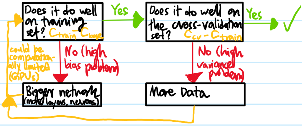
Problem: Draw a flow chart to illustrate a typical machine learning workflow:
Solution: It almost never hurts to go to a bigger neural network as long as one regularizes appropriately:
(bigger network = more features)
Problem: Explain the meaning of the phrase “large neural networks are low-bias machines“.
Solution: Loosely speaking, provided:
\[\text{Number of Neurons in Neural Network}\gg\#\mathcal D\]
then neural networks can almost always fit the training data pretty well, meaning low-bias. As a result, it is typically the case that high-variance is a bigger problem.
Problem: Describe what error analysis means in the context of evaluating a machine learning system’s classification performance (does it also apply to regression?)
Solution: The idea is that, if a neural network is diagnosed with high variance issues, rather than just feeding it more random training examples, one should feed it in a smarter way by first looking at the exact nature of the misclassifications.
Problem: Suppose a neural network is diagnosed with high variance, and error analysis shows that in fact one simply needs more training examples in general, but new training examples are scarce; in this case, what are \(2\) additional techniques one can try to improve the performance of one’s ML system?
Solution:
Data Augmentation: take existing training examples one already has, and perturb them in “representative” ways so as to obtain new training examples.
Data Synthesis: create new “representative” training examples out of thin air. There are many ways to do this depending on the specific application.
Problem: What are the \(2\) steps of transfer learning?
Solution:
Supervised Pretraining: train a neural network on a loosely related task.
Fine Tuning: taking the weights and biases of the hidden layers in the pretrained neural network as a starting point, do further training on either just the output layer or of the entire neural network, until it performs as desired on the task for which abundant data was not so immediately available.
Problem: Given a system of \(N\) identical bosons or fermions with Hamiltonian \(H\) in a mixed ensemble described by a density operator \(\rho\) (usually \(\rho=e^{-\beta H}/Z\) or \(\rho=e^{-\beta(H-\mu N)}/Z\) in equilibrium at temperature \(T=1/k_B\beta\) and chemical potential \(\mu\) though one can also work with a non-equilibrium \(\rho\); another limit often taken is \(T=0\) in which case the system is guaranteed to be in its ground state) and two operators \(P(t),Q(t)\) in the Heisenberg picture, define the greaterGreen’s function \(G^{>}_{P,Q}(t,t’)\), the lesser Green’s function \(G^{<}_{P,Q}(t,t’)\), the causal Green’s function \(G_{P,Q}(t,t’)\), the retarded Green’s function \(G^+_{P,Q}(t,t’)\), and the advanced Green’s function \(G^-_{P,Q}(t,t’)\) of \(P\) and \(Q\).
Solution: In all the formulas, the expectation is with respect to \(\rho\), (\(\langle A\rangle=\text{Tr}(\rho A)\) which at \(T=0\) looks like typical QFT expectations \(\langle \space|A|\space\rangle\) in a vacuum ground state \(|\space\rangle\)), and in all \(\pm,\mp\) occurrences, the “top” sign is for bosons while the “bottom” sign is for fermions:
\[G_{P,Q}(t,t’)=\Theta(t-t’)G^{>}_{P,Q}(t,t’)+\Theta(t’-t)G^{<}_{P,Q}(t,t’)=-\frac{i}{\hbar}\langle\mathcal T P(t)Q(t’)\rangle\]
(note that \(\mathcal T P(t)Q(t’)=\Theta(t-t’)P(t)Q(t’)\pm\Theta(t’-t)Q(t’)P(t)\) and in particular for fermions the time-ordering is not simply equal to \(\mathcal T P(t)Q(t’)\neq \Theta(t-t’)P(t)Q(t’)+\Theta(t’-t)Q(t’)P(t)\))
where \([A,B]_{-}=[A,B]\) is the commutator for bosons while \([A,B]_-=\{A,B\}\) is the anticommutator for fermions, i.e. \([A,B]_{\pm}=AB\pm BA\).
(comment about if \(H=H_0+V\) and using interaction picture instead of Heisenberg).
Problem: Show that if the Hamiltonian \(H\) is time-independent and the density operator \(\rho=\rho(H)\) is a function of \(H\) only (such as in equilibrium \(\rho=e^{-\beta H}/Z\)), then all \(5\) Green’s functions are a function of only the time difference \(t-t’\).
Solution: Clearly it suffices to show it for the greater and lesser Green’s functions. Specifically, for any \(2\) Heisenberg operators \(P(t),Q(t’)\), one has:
Since \(H\) is time-independent, the time-evolution operator is just \(e^{-iHt/\hbar}\) and hence the Heisenberg operators are \(P(t)=e^{iHt/\hbar}Pe^{-iHt/\hbar}\) and \(Q(t’)=e^{iHt’/\hbar}Qe^{-iHt’/\hbar}\) so:
and the claim follows. Thus, in such cases there is no harm in letting \(t’:=0\).
Problem: For single-particle Green’s functions, what are \(P(t)\) and \(Q(t)\) typically? What about for two-particle Green’s functions (and beyond)?
Solution: For single-particle Green’s functions (called such even though it’s really still a many-body object because it’s sensitive to the full Hamiltonian \(H\)), the standard case of interest is \(P(t)=c_i(t)\) and \(Q(t’):=c^{\dagger}_j(t’)\) where \(\{|i\rangle\}\) is a basis of the single-particle state space and \(c_i, c^{\dagger}_j\) are the annihilation and creation operators associated to \(|i\rangle\) and \(|j\rangle\) respectively. For example, if one is dealing with a bunch of electrons moving in \(\mathbf R^3\) and one chooses \(|i\rangle\equiv |\mathbf x,\sigma\rangle\), then the single-particle retarded Green’s function (thought of as a \(2\times 2\) matrix) can be written as:
Single-particle Green’s functions are also loosely referred to as two-point correlation functions. By extension, an example of a two-particle Green’s function might take \(P(t)=N_{\mathbf k}(t):=\sum_{\mathbf k’\sigma}c_{\mathbf k’+\mathbf k,\sigma}(t)c_{\mathbf k’\sigma}(t)\) and \(Q(t’)=N_{-\mathbf k}(t’)\) which would be a four-point correlation function.
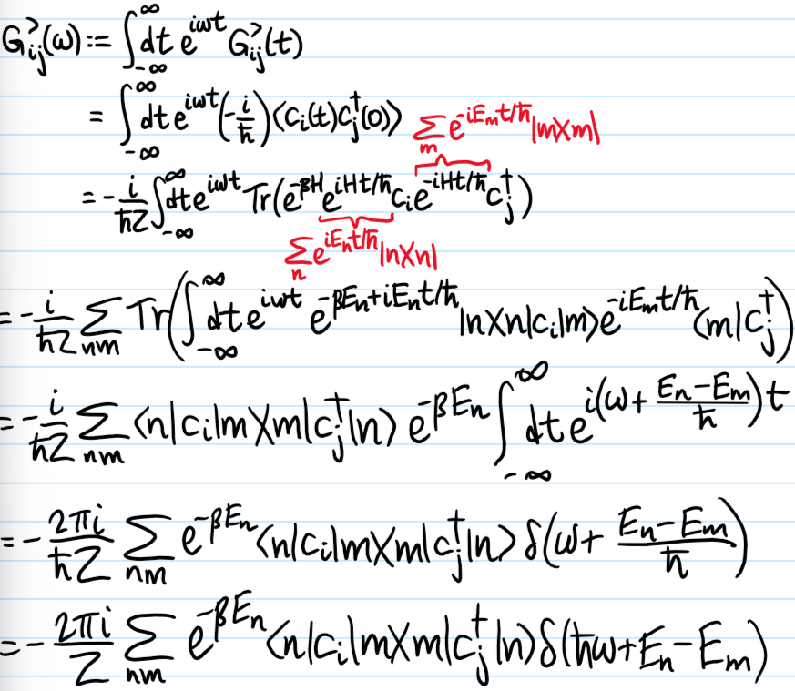
Problem: As mentioned earlier, when \(\rho=e^{-\beta H}/Z\) and \(\dot H=0\), one can set \(t’:=0\) without loss of information. In this case, being left with only a single time variable \(t\), one can Fourier transform each of the \(5\) single-particle Green’s functions from the time domain \(t\mapsto\omega\) to the frequency domain (with the usual linear response convention). In this case, show that the frequency-domain Green’s functions admit the Lehmann (also called spectral) representations:
where \(\{|n\rangle\}\) is an orthonormal \(H\)-eigenbasis.
Solution: (here the derivation was done with \(P=c_i\) and \(Q=c^{\dagger}_j\) but it works with arbitrary \(P,Q\)):
Problem: For each of the \(5\) frequency-domain Green’s functions (equilibrium \(\rho=e^{-\beta H}/Z\), time-independent \(H\) as before), one can define a corresponding spectral function. For instance, associated to the retarded Green’s function \(G_{P,Q}^+(\omega)\) is the retarded spectral function:
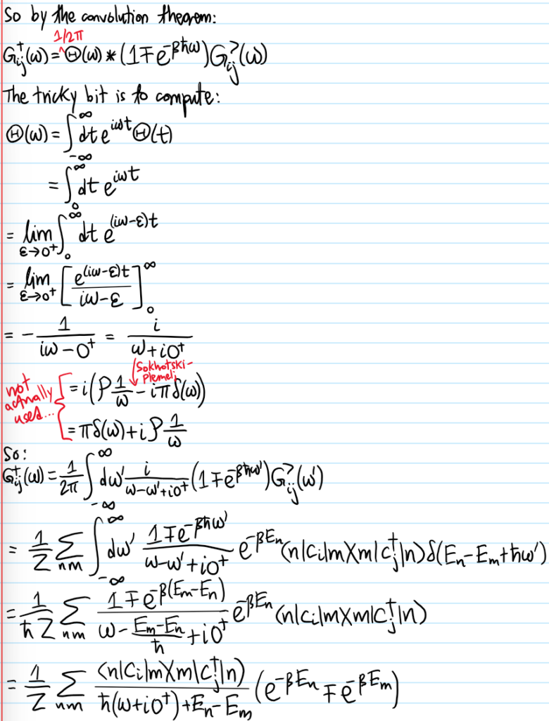
Show that, in the special but important case where \(Q=P^{\dagger}\), the corresponding retarded spectral function \(A^+_{P,P^{\dagger}}(\omega)\) scales with both the greater Green’s function \(G^>_{P,P^{\dagger}}(\omega)\) and the lesser Green’s function \(G^<_{P,P^{\dagger}}(\omega)\) in the frequency domain as:
where \(N_{\pm}(\omega):=\frac{1}{e^{\beta\hbar\omega}\pm 1}\) are respectively Bose-Einstein/Fermi-Dirac distributions. These relations go by the name of the fluctuation-dissipation theorem (valid at equilibrium!) because \(G^>\) and \(G^<\) are clearly a measure of fluctuations whereas the spectral function \(A^+\) measures dissipation by virtue of being \(\propto G^+\).
Solution: The quick and dirty way is to just use the Lehmann representation of \(G^+_{P,P^{\dagger}}(\omega)\), and when taking its imaginary part one just needs to invoke Sokhotski-Plemelj to get a bunch of \(\delta\)’s which makes it look very similar to the Lehmann representations of \(G^>_{P,P^{\dagger}}(\omega)\) and \(G^<_{P,P^{\dagger}}(\omega)\) from which the results follow.
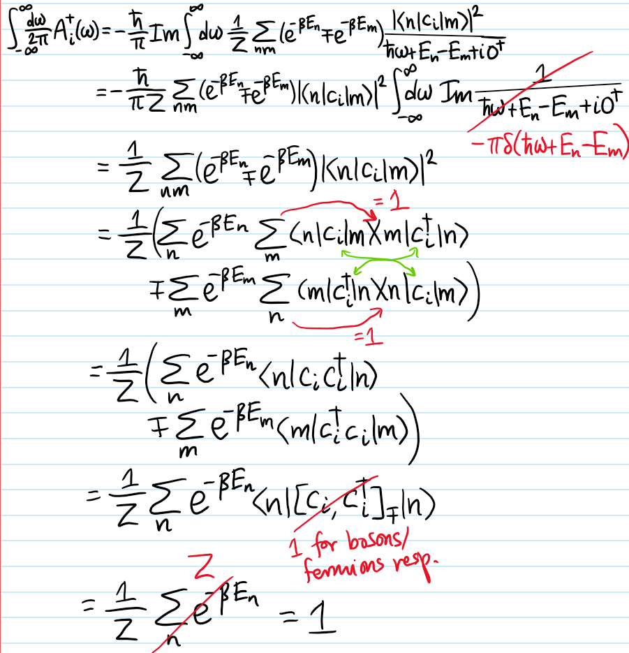
Problem: Specializing from the above problem, work with a diagonal component \(P=c_i\) of the single-particle retarded Green’s function. In this case, show that the retarded spectral function \(A^+_i(\omega)\) obeys the sum rule:
Solution: This is the first time that the commutation/anticommutation relation is actually necessary:
(note: in some literature, the spectral function is taken to be \(A^+_{P,Q}(\omega)=-\frac{\hbar}{\pi}\text{Im}G^+_{P,Q}(\omega)\) such that with this convention the sum rule reads \(\int_{-\infty}^{\infty}d\omega A^+_{P,Q}(\omega)=1\)).
Connect these to the resolvent of \(H\) and FT of time-evolution operator? (see the Oxford text for more)
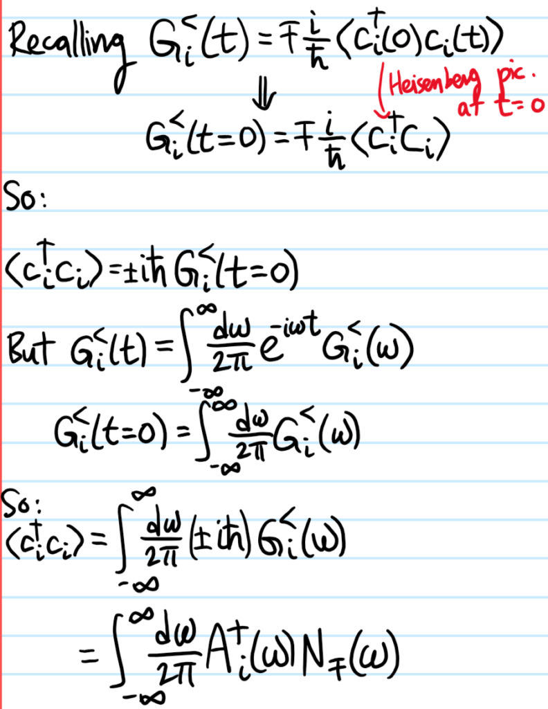
Problem: Show that the retarded spectral function \(A^+_i(\omega)\) behaves like a density of states:
Problem: For a system of non-interacting identical bosons/fermions, what is the (retarded) spectral function \(A^+_{\sigma}(\mathbf k,\omega)\)?
Solution: In that case, \(H=\sum_{\mathbf k\sigma}\frac{\hbar^2|\mathbf k|^2}{2m}c^{\dagger}_{\mathbf k\sigma}c_{\mathbf k\sigma}\). Although one can directly use the Lehmann representation formulas given that for both bosons and fermions the eigenstates \(|n\rangle\) and spectrum \(E_n\) of \(H\) are well-understood, it’s instructive to do a “first-principles” derivation. Specifically, first one needs to show that the the free time evolution of the creation and annihilation operators is explicitly given by:
The rigorous way is to simply downgrade from \(c_{\mathbf k\sigma}(t)=e^{iHt/\hbar}c_{\mathbf k\sigma}e^{-iHt/\hbar}\) back to the Heisenberg equation of motion \(i\hbar\dot c_{\mathbf k\sigma}(t)=[c_{\mathbf k\sigma}(t),H]=e^{iHt/\hbar}[c_{\mathbf k\sigma},H]e^{-iHt/\hbar}\) and upon inserting \(H=\sum_{\mathbf k’\sigma’}\frac{\hbar^2|\mathbf k’|^2}{2m}c^{\dagger}_{\mathbf k’\sigma’}c_{\mathbf k’\sigma’}\), recognize this as the commutator \([c_i,N_j]=\delta_{ij}c_i\) valid for both bosons and fermions (read it as a fancy way of saying \(N-(N-1)=1\)). This gives a \(1^{\text{st}}\)-order ODE for \(c_{\mathbf k\sigma}(t)\) with the trivial solution \(c_{\mathbf k\sigma}(t)=e^{-i\hbar |\mathbf k|^2t/2m}c_{\mathbf k\sigma}\), and by taking the adjoint one also gets \(c^{\dagger}_{\mathbf k\sigma}(t)=e^{-i\hbar |\mathbf k|^2t/2m}c^{\dagger}_{\mathbf k\sigma}\). The quicker, but more intuitively appealing way, is to directly take \(c_{\mathbf k\sigma}(t)=e^{iHt/\hbar}c_{\mathbf k\sigma}e^{-iHt/\hbar}\) and act on an arbitrary Fock state. The result then amounts to an identity of the form \(e^{i(E-\hbar^2|\mathbf k|^2/2m)t/\hbar}e^{-iEt/\hbar}=e^{-i\hbar|\mathbf k|^2t/2m}\). Armed with this, the diagonal retarded single-particle Green’s function is:
which reinforces that the Bose-Einstein/Fermi-Dirac distributions are strictly only valid for non-interacting systems of bosons/fermions.
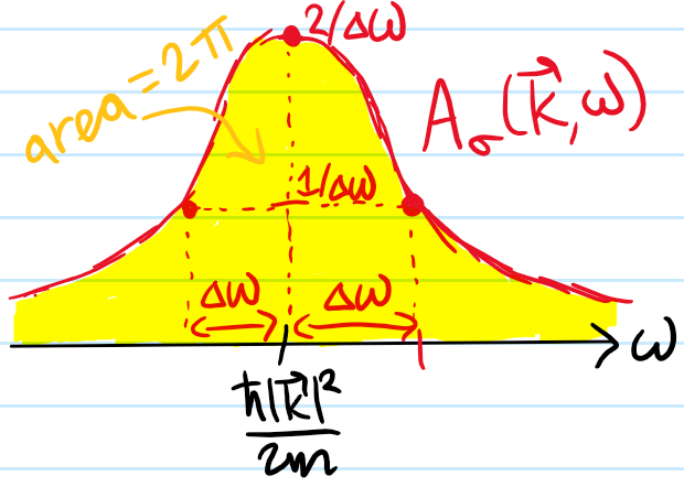
Problem: Above, the \(\varepsilon\)-prescription seemed to be a bit artificial…on the other hand, if one replaces \(\varepsilon\mapsto\Delta\omega\) so that the retarded Green’s function decays exponentially in time (due to interactions which scatter particles out of the state \(|\mathbf k\sigma\rangle\)) with non-infinitesimal decay rate \(\Delta\omega>0\), then show that the spectral function is broadened from a \(\delta\) spike into a Lorentzian with HWHM \(\Delta\omega\):
and the claim follows. Aside: if \(\Delta\omega\) is not too large, then this gives rise to the idea of a quasiparticle from Landau’s Fermi liquid theory. In that case, a generic spectral function might have the form:
where \(Z_{\mathbf k}\in[0,1]\) is a momentum-dependent quasiparticle residue and in particular if \(Z_{\mathbf k}\neq 1\) then an incoherent background/continuum spectrum \(\tilde A^+_{\sigma}(\mathbf k,\omega)\) must be present in order for \(A^+_{\sigma}(\mathbf k,\omega)\) to still obey the sum rule.
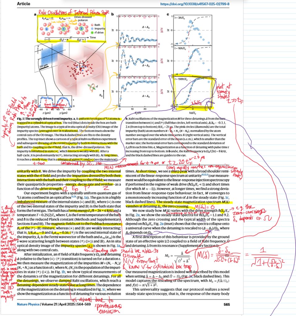
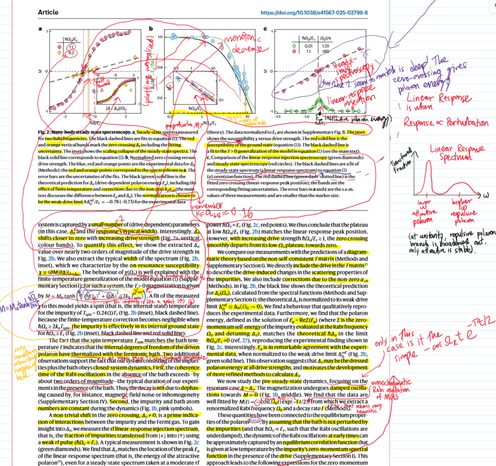
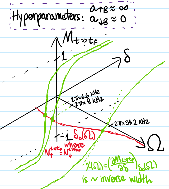
Everything in the first half of the paper (steady state part) can be summed up like:
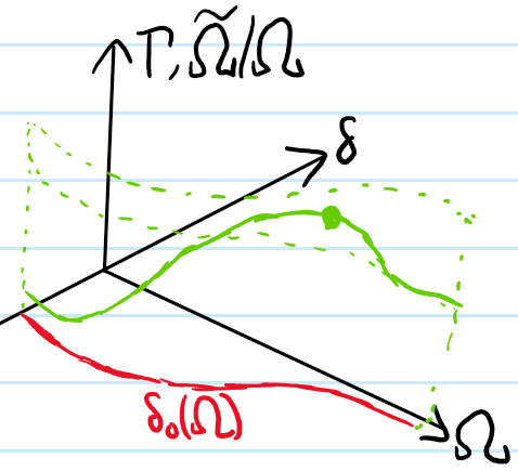
And the latter half discussing the resonant dynamics of the pre-steady state can be visualized qualitatively as:
Finally, a few points worth emphasizing:
Clearly \(\uparrow\) is unstable, wants to decay back to \(\downarrow\) with transition rate \(\Gamma\), so the zero-detuning \(\delta_0<0\) must contain information about the \(\uparrow,B\) interactions.
A Rabi experiment is different from say Ramsey in that it really is about a continuous drive so \(t\gg 1/\Omega\), as mentioned in the paper’s Figure \(1a\).
To emphasize again, there is the implicit hyperparameters that \(a_{\uparrow B}=\infty\) is unitarily/strongly interacting while \(a_{\downarrow B}\approx 0\) is weakly/non-interacting; the paper gives exact values). So only the attractive polaron is present. At the end the paper mentions extending into the BEC regime, where both would coexist for a sufficiently broad Feshbach resonance.
And some random thoughts I have about the paper:
Instead of the \(3D\) surface graph, maybe a heat map would be instructive too?
At large \(\Omega\), how does the AC Stark shift associated with a dressed atom-photon affect the physics (since it seems it would affect the internal energies of the polaron)?
Problem: Write an essay that summarizes the key points learned from the following papers/slides:
Solution: For a generic \(2\)-component Fermi gas whose \(2\) components may be called \(\uparrow\) and \(\downarrow\) (this could be \(2\) hyperfine states of the same atom, or \(2\) hyperfine states of different atoms) the Hamiltonian is \(H=H_0+V_{\downarrow\uparrow}\) where the kinetic energy is:
and the short-range scattering pseudopotential \(V_{\downarrow\uparrow}\) of “bare strength” \(g_{\uparrow\downarrow}\) describes momentum-conserving collisions between the \(2\) components \(\uparrow,\downarrow\) of the Fermi gas in a volume \(V\) (note that interactions among the components themselves are neglected, i.e. they are separately ideal Fermi gases. That is, one assumes there is no \(\uparrow\uparrow\) or \(\downarrow\downarrow\) scattering. This is justified by the fact that identical spin parts of \(2\) identical fermions could only interact via an odd-\(\ell\) scattering channel, the lowest of which is \(\ell=1\) \(\p\)-wave scattering whose cross-section \(\sigma_{\ell}\sim k^{2\ell}\) is suppressed at low \(k\)):
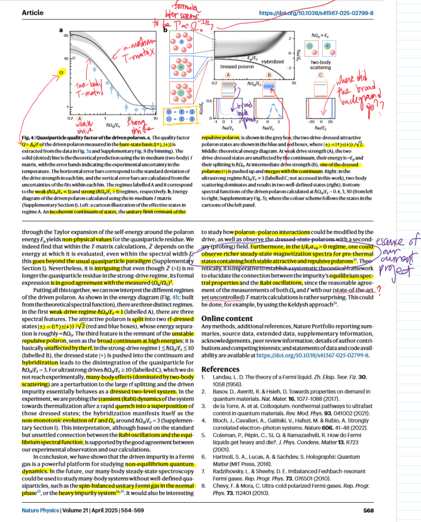
The Fermi polaron is the limit \(N_{\downarrow}/N_{\uparrow}\to 0\) of the \(2\)-component Fermi gas, in fact typically one just takes \(N_{\downarrow}=1\). In light of this population imbalance between the \(2\) components \(\uparrow,\downarrow\) of the Fermi gas, the standard terminology is to call the majority \(\uparrow\) component as the bath and the minority \(\downarrow\) component as the impurity. Through the short-range interaction \(V_{\downarrow\uparrow}\), the \(\downarrow\) impurity polarizes the \(\uparrow\) bath in its \(\textbf x\)-space vicinity (hence the name polaron!), and it is common to say that the \(\downarrow\) impurity is dressed by the polarized \(\uparrow\) cloud that it “carries” along with it. This composite object of the \(\downarrow\) impurity together with the \(\uparrow\) cloud is a quasiparticle called the (Fermi) polaron (in particular, it is important to emphasize that polaron is not synonymous with \(\downarrow\) impurity; the interaction \(V_{\downarrow\uparrow}\) is essential and instead polaron is synonymous with \(\downarrow\) impurity + \(\uparrow\) polarized cloud).
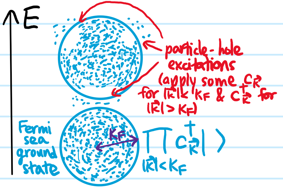
This discussion has been an intuitive/qualitative picture in \(\textbf x\)-space (aka real space). In \(\textbf k\)-space (aka reciprocal space), one can get more quantitative. Here, rather than starting from a \(2\)-component \(\uparrow\downarrow\) Fermi gas, one can first visualize a single-component \(\uparrow\) ideal Fermi gas in its ground state where the Fermi sea is occupied up to the Fermi wavenumber \(k_F=(6\pi^2 n_{\uparrow})^{1/3}\):
The excited states are then particle-hole excitations of this ground state Fermi sea \(|\text{FS}\rangle\). When adding a single \(\downarrow\) impurity to the bath, one would expect that the impurity would scatter bath fermions from inside to outside the Fermi sea. The modifiedground state \(|\text{FP}\rangle\) of the Fermi polaron system (i.e. the \(\downarrow\) impurity + \(\uparrow\) bath) would therefore be expected to be of the form (working in the ZMF classically, or quantum mechanically fixing an eigenstate of total momentum \(\textbf 0\)):
where the \(…\) indicates \(N\) particle-hole excitations for \(N\geq 2\). Ignoring the \(…\) terms, this is called the Chevy ansatz and can be used as a trial ground state with \(\alpha_0,\alpha_{\textbf k,\textbf k’}\) the fitting parameters to be tuned such as to minimize the Rayleigh-Ritz energy quotient \(E=\frac{\langle\text{FP}|H|\text{FP}\rangle}{\langle \text{FP}|\text{FP}\rangle}\) in the variational method. The ground state energy eigenvalue \(E\) obtained in this manner is an estimate of the polaron energy. Explicitly:
As another corollary, the fitting parameter \(\alpha_0\), once fitted, gives the polaron residue:
\[Z:=|\alpha_0|^2\leq 1\]
The (unobservable) bare strength \(g_{\uparrow\downarrow}=g_{\uparrow\downarrow}(k^*)\) should be taken to run with the (unobservable) UV cutoff \(k^*\to\infty\) such as to keep \(a_s\) fixed! Specifically, through the renormalization condition:
But \(\psi(\textbf x)=e^{ikz}+f(\textbf k,\textbf k’)\frac{e^{ikr}}{r}\), and it’s that divergent \(1/r\) piece in the scattered spherical wave that’s gonna cause trouble. This is because \(\psi(\textbf 0)\) seems to blow up due to it. But rather than let it blow up, allow it to be some large number call it \(k^*/\pi\) (clearly dimensionally okay). Then \(\psi(\textbf 0)=1+f(\textbf k,\textbf k’)k^*/\pi\). Substituting gives and isolating for \(f\):
The point is now, suddenly, you introduce a new low-energy parameter into the game, the \(s\)-wave scattering length \(a_s\)! Notice it didn’t appear in any equations yet! But since we only care about low-energy/low-momentum \(\textbf k\to\textbf 0\), and we know we have the limit \(f(\textbf k,\textbf k’)\to -a_s\) as \(\textbf k\to \textbf 0\). It’s a sort of limit/correspondence principle-like knot at the end of a string that the theory has to approach. So making that substitution, one obtains the running of the bare coupling with the UV cutoff. This turns out the be the same as the above renormalization condition.
More precise derivation:
Write the Born series for the scattering amplitude:
By defining the transition operator \(T_{\uparrow\downarrow,s}|\textbf k\rangle:=V_{\uparrow\downarrow,s}|\psi_{\textbf k}\rangle\) which can be easily checked to obey \(T=V+VG_0T\) with \(G_0=(E_{\textbf k}1-H_0)^{-1}\) the free particle resolvent, then because \(\langle k|V_{\uparrow\downarrow,s}|\textbf k’\rangle=g\) for \(V_{\uparrow\downarrow,s}=g\delta^3(\textbf X)\), then actually \(\textbf k’\) doesn’t even matter (i.e. \(s\)-wave scattering is isotropic!) so it can be used as a dummy index for the summation. Furthermore to the isotropy, \(f(\textbf k)=f(k)\):
In the end, once you set \(\textbf k:=\textbf 0\) so that \(f(0)=-a_{\uparrow\downarrow,s}\), you get the same thing. Here, the subtleties are that the series part can be summed by letting \(V\to\infty\) so \(\frac{1}{V}\sum_{\textbf k’}\to\int\frac{d^3\textbf k’}{(2\pi)^3}\), and if you take \(\langle\textbf x|\textbf k\rangle=e^{i\textbf k\cdot\textbf x}\) then the correct identity resolution is \(\frac{1}{V}\sum_{\textbf k}|\textbf k\rangle\langle\textbf k|\) for quantization volume \(V\) and also remember \(G_0|\textbf k’\rangle=\frac{1}{E_{\textbf k}-E_{\textbf k’}}|\textbf k’\rangle\) is an eigenstate.
(there are both attractive and repulsive Fermi polarons so this polarization effect can go either way). In the attractive case, if the attraction is strong enough, the the polaron can dimerize with a bath fermion, forming a molecule; this polaron-molecule transition is interesting.
Surprisingly, the Chevy ansatz works remarkably well (i.e. agrees with state-of-the-art diagrammatic quantum Monte Carlo stuff)! Seems to include the dimer bound state in it?
———————-
There are \(2\) key assumptions about the typical regime of ultracold atomic gases, namely \(n^{-1/3},\lambda_T\gg r_{vdW}\sim 100a_0\).
In the vicinity of a broad Feshbach resonance, the scattering amplitude may be approximated by the Mobius transformation \(f_s(k)=-\frac{1}{ik+a^{-1}_s}\). However, in the vicinity of a narrow Feshbach resonance, need to also parameterize it with the effective range \(r_{\text{eff}}\) so that \(f_s(k)=-\frac{1}{ik+a^{-1}_s-\frac{1}{2}r_{\text{eff}}k^2}\). Although \(a_s\) and \(r_{\text{eff}}\) are determined by microscopic details of \(V_{\uparrow\downarrow}(r)\), different microscopic details in another potential \(\tilde V_{\uparrow\downarrow}(r)\) can lead to the same low-energy scattering amplitude \(f_s(k)\). The practical corollary of this observation is that one do just that, namely substitute \(V_{\uparrow\downarrow}(r)\) for a suitable pseudopotential.
Problem: Consider a toy model of the Fermi polaron in which the \(\downarrow\) impurity interacts with only the nearest \(\uparrow\) impurity in the Fermi sea, the rest of the \(\uparrow\) Fermi sea serving to exert a pressure that effectively confines the relative distance between the \(\downarrow\) and \(\uparrow\) impurities to a radius \(R\). By equating the ground state energy of the infinite spherical potential well with the Fermi energy \(E_F\), show that:
\[R=\sqrt{\frac{m_{\uparrow}}{\mu}}\]
Hence, show that for a positive-energy eigenstate \(E=\frac{\hbar^2k^2}{2m}\) the wavenumber \(k\) is determined through the \(s\)-wave scattering length \(a_s\) by:
\[k\cot kR=a^{-1}_s+R^*k^2\]
(where the Bethe-Peierls boundary condition is used). Show that for \(m_{\uparrow}=m_{\downarrow}\) and \(R^*=0\), this simplifies to:
By considering the scaled energy from the Fermi energy \(\frac{E-E_F}{E_F}\) which in this case amounts to \(2(k/k_F)^2-1\), plot this as a function of \(-1/k_Fa_s\).
Problem: Explain how Ramsey interferometry works.
Solution: Applying two \(\pi/2\)-pulses separated by some time \(\Delta t\); then Ramsey fringes are seen as a function of this temporal separation \(\Delta t\); it is a bit like a time-domain analog of a Mach-Zender interferometer.
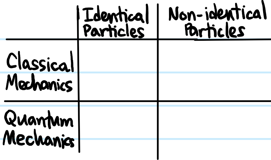
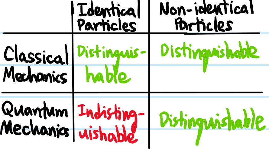
Problem: What does it mean for \(N=2\) particles to be identical?
Solution: \(N=2\) particles are identical iff their intrinsic properties are all identical; in classical mechanics this typically means mass \(m\), charge \(q\), etc. while in quantum mechanics this typically means mass \(m\), charge \(q\), and spin \(s\) (and other intrinsic quantum numbers). The word intrinsic is important here. For example, \(2\) electrons are considered identical classical particles even if they are at different positions \(\textbf x_1\neq\textbf x_2\), or travelling with different velocities \(\dot{\textbf x}_1\neq\dot{\textbf x}_2\), and likewise are considered identical quantum particles even if they are in different quantum states \(|n,\ell,m_{\ell},m_s\rangle\neq |n’,\ell’,m_{\ell’},m_{s’}\rangle\) for instance (although exactly what properties qualify as “intrinsic” isn’t obvious a priori…)
Problem: Fill in the \(4\) entries of the following \(2\times 2\) matrix with either the word distinguishable or indistinguishable.
Solution:
Problem: Consider \(N=2\) identical quantum particles, thus described by a state in \(\mathcal H^{\otimes 2}\), where \(\mathcal H\) is each of their (identical) single-particle state space. Define the exchange operator \((12):\mathcal H^{\otimes 2}\to \mathcal H^{\otimes 2}\).
Solution: For some reason the term “exchange” is conventional in the QM literature even though the term “transposition” is usually used to describe this (e.g. in group theory). For unentangled states, the exchange operator is defined by:
where \(|\psi\rangle,|\phi\rangle\in\mathcal H\) are arbitrary single-particle states, and extended to the rest of \(\mathcal H^{\otimes 2}\) by linearity. In particular, transposition is manifestly independent of one’s choice of \(\mathcal H\)-basis because this definition doesn’t mention any \(\mathcal H\)-basis.
Problem: Show that \((12)\) is both unitary and Hermitian; hence what are the eigenvalues of \((12)\) and give an example of an eigenstate with each eigenvalue.
Solution:
The eigenvalues of \((12)\) are thus \(\text{spec}(12)=\{-1,1\}\). For example, \((12)|\psi\rangle\otimes|\psi\rangle=|\psi\rangle\otimes|\psi\rangle\) has eigenvalue \(1\) for any \(|\psi\rangle\in\mathcal H\). By contrast, \((12)(|\psi\rangle\otimes|\phi\rangle-|\phi\rangle\otimes|\psi\rangle)=-(|\psi\rangle\otimes|\phi\rangle-|\phi\rangle\otimes|\psi\rangle)\) has eigenvalue \(-1\) for any \(|\psi\rangle,|\phi\rangle\in\mathcal H\)
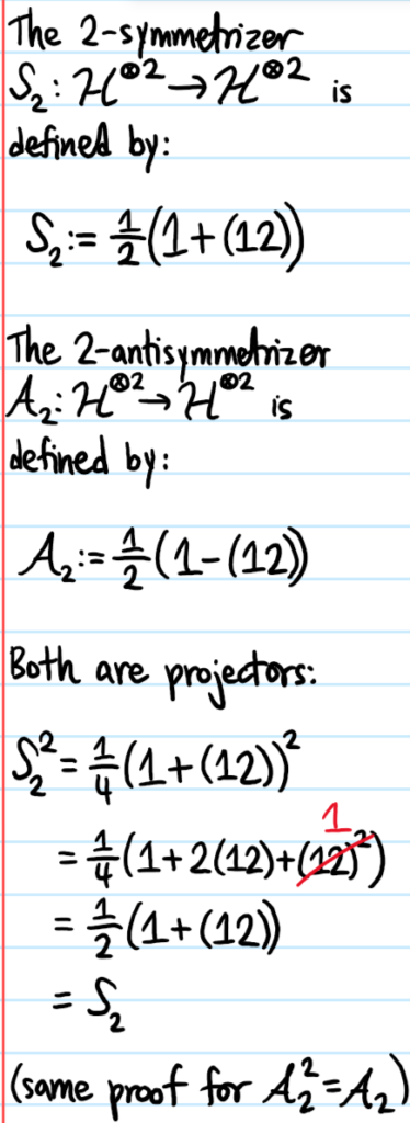
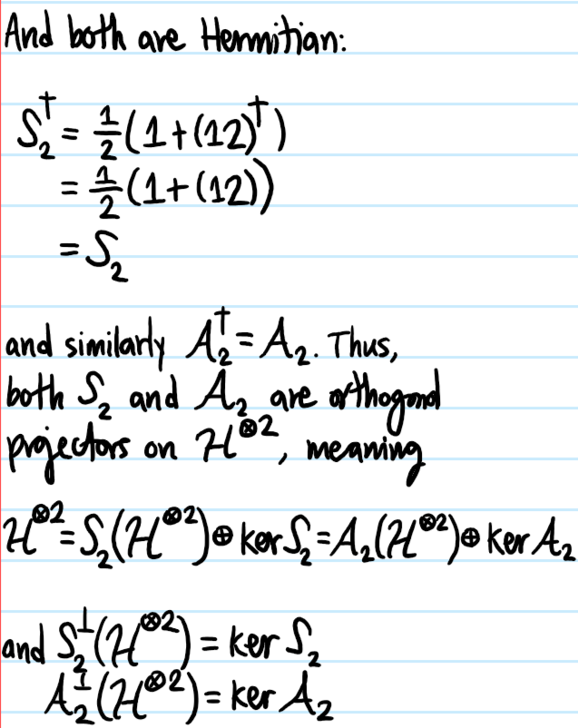
Problem: Define the \(2\)-symmetrizer \(\mathcal S_2\) and the \(2\)-antisymmetrizer \(\mathcal A_2\) and show that both are orthogonal projectors.
Solution:
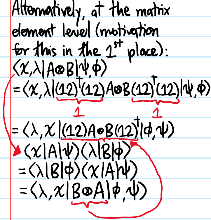
Problem: Let \(A,B:\mathcal H\to\mathcal H\) each be arbitrary linear operators on the single-particle state space \(\mathcal H\). The exchange operator acts on states by a unitary \((12)\) which swaps \(|\psi\rangle\otimes|\phi\rangle\mapsto|\psi\rangle\otimes|\phi\rangle\). If one wished to achieve an analogous result at the level of operators, specifically \(A\otimes B\mapsto B\otimes A\), how can this be accomplished?
Solution:
Problem: Generalizing the above slightly, given arbitrarily many compositions of operators on \(\mathcal H^{\otimes 2}\), e.g. \((A\otimes B)(C\otimes D)(E\otimes F)…\), how can one obtain the operator \((B\otimes A)(D\otimes C)(F\otimes E)…\)?
Problem: Show that an operator \(\mathcal O:\mathcal H^{\otimes 2}\to\mathcal H^{\otimes 2}\) is exchange-symmetric iff \([\mathcal O,(12)]=0\).
Solution: In light of the above, an exchange-symmetric operator is reasonably defined to obey:
\[(12)\mathcal O(12)^{-1}=\mathcal O\]
and hence the result follows.
(aside: all of the above discussion also holds for \(2\) non-identical quantum particles provided one assumes they are each described by the same single-particle state space \(\mathcal H\)).
Now, generalize the prior discussion to an arbitrary number \(N\) of identical quantum particles.
Problem: Define the \(N\)-symmetrizer \(\mathcal S_N\) and the \(N\)-antisymmetrizer \(\mathcal A_N\) operators on the space \(\mathcal H^{\otimes N}\) of \(N\) identical particles (where \(\mathcal H\) as before is the single-particle state space).
where \(\#S_N=N!\), and note this is consistent with the earlier definitions for \(N=2\). Strictly speaking each permutation \(\sigma\in S_N\) is an abstract group element for which there is no notion of “group addition”, rather this is a faithful unitary representation of \(S_N\) on \(\mathcal H^{\otimes N}\) (a more pedantic notation could be \(\hat{\sigma}\) for the permutation operator associated to \(\sigma\)).
Problem: Establish the following properties of \(\mathcal S_N\) and \(\mathcal A_N\):
i) (Useful lemma) \[\sigma\mathcal S_N=\mathcal S_N\sigma=\mathcal S_N\] and \[\sigma\mathcal A_N=\mathcal A_N\sigma=\text{sgn}(\sigma)\mathcal A_N\] for any \(\sigma\in S_N\).
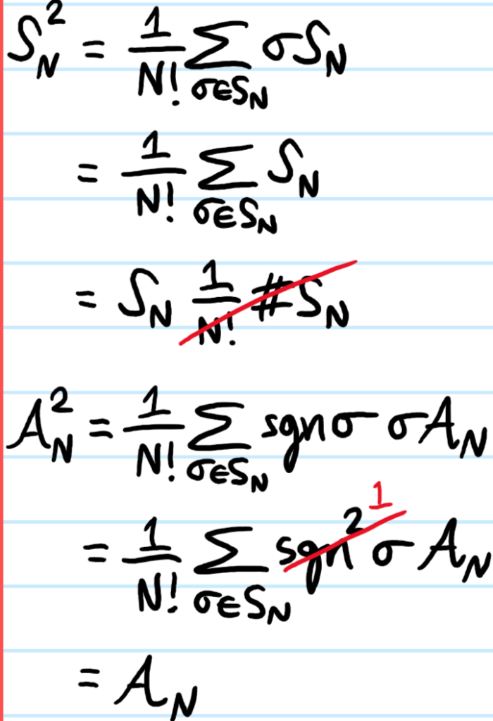
ii) (Orthogonal projectors) \(\mathcal S^2_N=\mathcal S_N\) and \(\mathcal A^2_N=\mathcal A_N\) are both idempotent projections, and \(\mathcal S^{\dagger}_N=\mathcal S_N\) and \(\mathcal A^{\dagger}_N=\mathcal A_N\) are both Hermitian observables.
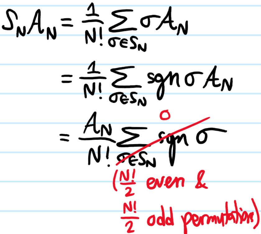
iii) (Orthogonal images) \(\mathcal S_N\mathcal A_N=\mathcal A_N\mathcal S_N=0\) (but note this is in general not a full orthogonal complement, i.e. \((\mathcal S^{\perp}_N(\mathcal H^{\otimes N})\neq\mathcal A_N(\mathcal H^{\otimes N})\) unless \(N=2\); in other words, for \(N\geq 3\), there exist states that are neither symmetric nor antisymmetric, but have mixed symmetries, see Young tableaux).
Solution:
i) Since \(S_N\) is a normal subgroup of itself, its left/right cosets coincide and indeed, all simply return \(S_N\) trivially. For \(\mathcal A_N\), one can write:
and since \(\text{sgn}:S_N\to\{-1,1\}\) is a homomorphism, this simplifies to the claimed result.
ii) First, note that (as mentioned above), all permutations \(\sigma\in S_N\) are unitary (this follows because all permutations can be built from transpositions alone, each of which was proven to be unitary from the \(N=2\) analysis earlier). Thus, taking the adjoint is the same as the inverse. So:
but \(S_N\) is a group, so inversion is a group bijection, and the sum is invariant. For \(\mathcal A_N\), the proof of Hermiticity is almost identical with the additional insight that inversion also preserves the sign \(\text{sgn}(\sigma^{-1})=\text{sgn}(\sigma)\) since any decomposition into transpositions would just be reversed, but the number of transpositions (even/odd) would be invariant. Regarding projection:
iii) For example:
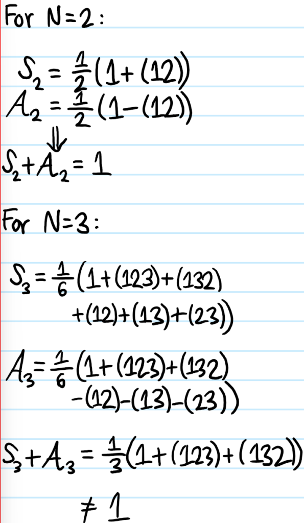
Problem: Following up on the above iii), show explicitly that for \(N=2\) identical particles, \(S_2+A_2=1\) partitions the space \(\mathcal H^{\otimes 2}\) but for \(N=3\) identical particles \(S_3+A_3\neq 1\).
Solution: (it seems the reason it breaks down is basically because for \(N\geq 3\), the identity permutation is no longer the only even permutation)
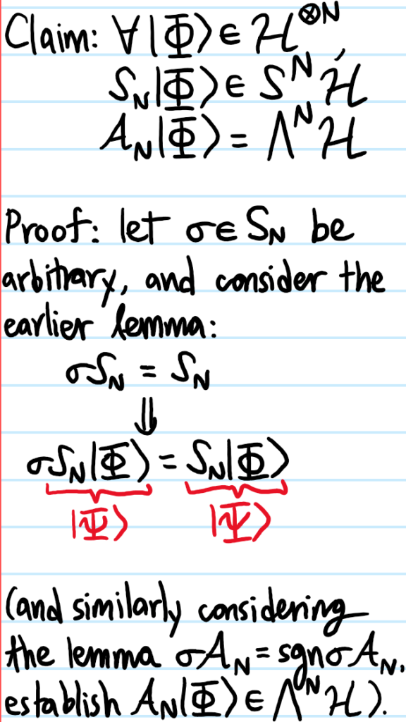
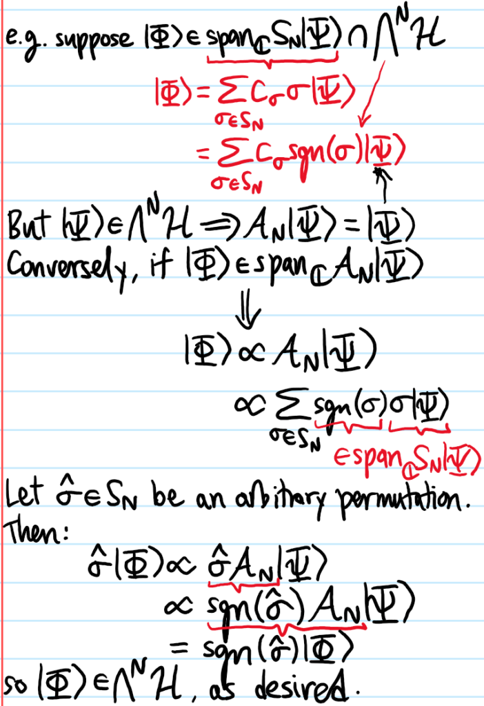
Problem: Define the totally symmetric state subspace \(S^N\mathcal H\) and the totally antisymmetric state subspace \(\bigwedge^N\mathcal H\) of the full \(N\)-particle state space \(\mathcal H^{\otimes N}\) and hence explain why the \(N\)-symmetrizer \(\mathcal S_N:\mathcal H^{\otimes N}\to S^N\mathcal H\) and the \(N\)-antisymmetrizer \(\mathcal A_N:\mathcal H^{\otimes N}\to \bigwedge^N\mathcal H\) may be viewed thus.
Solution: The totally symmetric state subspace is essentially the intersection of the eigenspaces of all permutation operators with eigenvalue \(1\) (or in group-theoretic language, the set of all states whose stabilizer subgroup is \(S_N\) itself):
\[S^N\mathcal H:=\{|\Psi\rangle\in\mathcal H^{\otimes N}:\sigma|\Psi\rangle=|\Psi\rangle\text{ for all }\sigma\in S_N\}\]
(permutation operators do not commute as one can see from the conjugacy classes of \(S_N\), so they cannot all be simultaneously diagonalized, but nevertheless it turns out to still be possible to find special symmetric states that are eigenstates of all of them). The totally antisymmetric state subspace is defined by:
\[\bigwedge^N\mathcal H:=\{|\Psi\rangle\in\mathcal H^{\otimes N}:\sigma|\Psi\rangle=\text{sgn}(\sigma)|\Psi\rangle\text{ for all }\sigma\in S_N\}\]
Problem: State the symmetrization postulate of quantum mechanics.
Solution: For a system of \(N\) identical quantum particles, not all states in \(\mathcal H^{\otimes N}\) are physical states, even though they may be valid “mathematical states”. Instead, only states in \(S^N\mathcal H\) xor states in \(\bigwedge^N\mathcal H\) can be physical states, corresponding respectively to identical bosons vs. identical fermions.
Problem: Show that for any \(N\)-body state \(|\Psi\rangle\in\mathcal H^{\otimes N}\), the symmetrization of \(|\Psi\rangle\) obtained by acting with the \(N\)-symmetrizer \(\mathcal S_N|\Psi\rangle\) is unique in the projective totally symmetric state subspace \(PS^N\mathcal H\), and similarly the antisymmetrization of \(|\Psi\rangle\) obtained by acting with the \(N\)-antisymmetrizer \(\mathcal A_N|\Psi\rangle\) is unique in \(P\bigwedge^N\mathcal H\).
For example, for the \(2^{\text{nd}}\) assertion above:
and the proof the first one is similar. Intuitively, any linear combination of permutations which is symmetric must in fact give uniform weight to all permutations (which is what \(\mathcal S_N\) prescribes), and similarly if the linear combination is antisymmetric, then each permutation is weighted by its sign instead (as per \(\mathcal A_N\)).
Problem: Let \(\{|1\rangle,|2\rangle,…\}\subseteq\mathcal H\) be an orthonormal basis of the single-particle state space \(\mathcal H\), and consider \(N\) identical particles living collectively in \(\mathcal H^{\otimes N}\). Explain why it is useful to introduce the notation \(|N_1,N_2,…,\rangle\) (called the occupation number representation) to denote that there are \(N_i\in\textbf N\) particles in single-particle state \(|i\rangle\in\mathcal H\).
Solution:Because the particles are identical, it is highly inefficient to be asking “which state is which particle in” since the notion of “which particle” is meaningless. Instead, common sense dictates that the more efficient question to ask is “how many particles are in each state?” as this doesn’t care about which particle is which.
Problem: If one demands \(\langle N_1,N_2,…|N_1,N_2,…\rangle=1\) to be normalized, then write down a single unified formula for \(|N_1,N_2,…\rangle\) in the language of first quantization that works regardless of whether the particles are identical bosons or identical fermions.
Solution: A little bit of thought shows that one possibility is:
where \(N=N_1+N_2+…\), and the \(\pm\) should be taken as \(+\) for bosons and \(-\) for fermions. If it’s for \(N\) identical bosons, one can write it in terms of the \(N\)-symmetrizer:
while for \(N\) identical fermions, the Pauli exclusion principle enforces \(N_i\in\{0,1\}\) for all single-particle states \(|i\rangle\), and thus \(N_i!=1\). Thus, in this case:
One can explicitly check the normalization of the state written in this manner:
Problem: Consider a system of \(3\) hydrogen atoms, \(2\) of which are in a single-particle ground state \(|0\rangle\) and \(1\) of them is in some single-particle excited state \(|1\rangle\); write down the \(3\)-body collective state of this system in first quantization.
Solution: Phrases like “ground state” and “excited state” are simply particular eigenstates of the single-particle Hamiltonian \(H\); in particular, because \(H\) is Hermitian, these single-particle states may be taken orthonormal. With this in mind, because hydrogen atoms are bosons (assuming the usual protium isotope without neutrons), the occupation number state \(|N_{|0\rangle}=2,N_{|1\rangle}=1\rangle\) is given in first quantization by:
where of course the shorthand \(|001\rangle:=|0\rangle\otimes |0\rangle\otimes |1\rangle\), etc. is being used.
Problem: All of the above discussion is always prefaced by fixing the number of identical quantum particles \(N\); in other words, all of the physics happens inside the \(N\)-particle sector of the Fock space \(\mathcal F_{\mathcal H}\) generated by the single-particle state space \(\mathcal H\). Define the Fock space \(\mathcal F_{\mathcal H}\) for identical bosons, and separately for identical fermions.
Solution: For both bosons and fermions, one can write:
(in fact the fermionic Fock space can also be written \(\mathcal F_{\mathcal H}=\bigoplus_{N=0}^{\dim\mathcal H}\bigwedge^N\mathcal H\) since for \(N>\dim\mathcal H\), the totally antisymmetric state space \(\bigwedge^N\mathcal H=\{0\}\) is trivial).
Problem: Explain why the Fock space \(\mathcal F_{\mathcal H}\) needs to be formed by a direct sum \(\oplus_{N=0}^{\infty}\) rather than just a union \(\bigcup_{N=0}^{\infty}\). Furthermore, explain how to complete Fock space \(\mathcal F_{\mathcal H}\) into a Hilbert space by explicitly stating the inner product placed on \(\mathcal F_{\mathcal H}\).
Solution: Simply put, the union \(\bigcup_{N=0}^{\infty}\) doesn’t preserve the vector space structure, hence the need for the direct sum \(\oplus_{N=0}^{\infty}\). The canonical inner product on \(\mathcal F_{\mathcal H}\) is defined by summing the inner product between respective components in the \(N\)-particle sectors (this statement is just a general property of direct sums in linear algebra).
Problem: Clarify by the above discussion by working through the example of electrons fixed in space, so that \(\mathcal H\cong\textbf C^2\). Let \(|0\rangle,|1\rangle\) be an orthonormal basis for \(\mathcal H\). What is the electron Fock space \(\mathcal F_{\mathcal H}\)? What is its dimension \(\dim(\mathcal F_{\mathcal H})\)? What is a basis for \(\mathcal F_{\mathcal H}\)? Hence, show that distinct \(N\)-particle sectors are orthogonal.
Solution:
in particular, it is clear that distinct \(N\)-particle sectors are orthogonal because the Fock states here \(|\space\rangle,|0\rangle,|1\rangle,\frac{|01\rangle-|10\rangle}{\sqrt{2}}\) form an orthonormal basis for \(\mathcal F_{\mathcal H}\cong\textbf C^4\). Note that both \(|\Psi\rangle,|\Phi\rangle\) will (in general) not be called Fock states because they do not contain a fixed number of particles \(N\), but rather are said to be in a superposition of Fock states, each of which by definition only deals with a fixed number \(N\) of particles in some \(N\)-particle sector (which is why it could be written using a single occupation number ket).
Problem: Outside of QFT, particles are conserved \(\dot N=0\), so it’s not obvious why one would ever want to somehow “tamper” with the number of particles \(N\) in the system. Nevertheless, it turns out to be very useful, like a magician waving their magic wand to make rabbits appear or disappear from their hat. Explain how the creation and annihilation operators for bosons and fermions are defined respectively on the bosonic and fermionic Fock spaces \(\mathcal F_{\mathcal H}\).
Solution: For a given single-particle basis \(\{|i\rangle\}\subset\mathcal H\) of the single-particle state space \(\mathcal H\), to each single-particle basis ket \(|i\rangle\), one associates a creation operator \(a^{\dagger}_i:\mathcal F_{\mathcal H}\to\mathcal F_{\mathcal H}\) and similarly an annihilation operator \(a_i:\mathcal F_{\mathcal H}\to\mathcal F_{\mathcal H}\). Since Fock states \(|N_1,N_2,…,\rangle\) form a basis for the Fock space \(\mathcal F_{\mathcal H}\), to define the action of each \(a^{\dagger}_i,a_i\) on the full Fock space \(\mathcal F_{\mathcal H}\), it suffices to define their actions on each Fock state, and extend to the rest of \(\mathcal F_{\mathcal H}\) by linearity. Hence, they are defined to act on Fock states via:
However, one should check that these \(2\) definitions are compatible in the sense that the claimed adjoint relation between \(a^{\dagger}_i\) and \(a_i\) is really correct w.r.t. the Fock space inner product. To this end, one has to check that for arbitrary \(|\Psi\rangle,|\Phi\rangle\in\mathcal F_{\mathcal H}\):
but bilinearity of the inner product means it suffices to check this when \(|\Psi\rangle=|N_1,N_2,…,N_i,…\rangle\) and \(|\Phi\rangle=|N’_1,N’_2,…,N’_i,…\rangle\) are both Fock states:
i) Write down a formula for a generic Fock state \(|N_1,N_2,…,\rangle\) in terms of creation operators acting on the vacuum \(|\space\rangle=|N_1=0,N_2=0,…\rangle\).
ii) Explain why, for any single-particle state \(|i\rangle\in\mathcal H\), the \(\alpha=0\) coherent state is given by:
iii) Evaluate for bosons the commutators \([a_i,a_j],[a^{\dagger}_i,a^{\dagger}_j],[a_i,a^{\dagger}_j]\) and for fermions the anticommutators \(\{c_i,c_j\},\{c^{\dagger}_i,c^{\dagger}_j\},\{c_i,c^{\dagger}_j\}\) (for fermions it is conventional to use the letter “\(c\)” in lieu of “\(a\)”).
iv) Given \(2\) single-particle bases \(\{|i\rangle\}\) and \(\{|\tilde i\rangle\}\) for the single-particle state space \(\mathcal H\), explain how to relate \(a^{\dagger}_i\) with \(a^{\dagger}_{\tilde i}\) and similarly how to relate \(a_i\) with \(a_{\tilde i}\). Verify that these transformations preserve the commutation/anticommutation relations.
v) Define the number operator \(\hat N_i\) and show that when acting on a Fock state, it counts the number of identical particles in the single-particle state \(|i\rangle\) (in fact, a good way to think about Fock states is that they are eigenstates of the total number operator \(\hat N:=\sum_i\hat N_i\)).
Solution:
i) In second quantization, the Fock state is given by:
\[|N_1,N_2,…,\rangle=\]
ii)
iii)
iv) Although it is tempting to think of this as a “change of basis” from linear algebra, this is actually not what’s going on…(or is it?)
v)
Problem: For \(\mathcal H=L^2(\textbf R^3\to\textbf C)\), one can use either the orthonormal \(\textbf X\)-eigenbasis \(\{|\textbf x\rangle\}\) or the orthonormal\(\textbf P\)-eigenbasis \(\{|\textbf k\rangle\). Show that the corresponding creation and annihilation operator fields for each are related by a Fourier transform:
where the notation \(\psi(\textbf x):=a_{\textbf x}\) and \(\psi_{\textbf k}:=a_{\textbf k}\) is being used (unambiguous with the wavefunction because this is \(2^{\text{nd}}\) quantization now! No more \(1^{\text{st}}\) quantization).
Problem: Consider a system of \(N=2\) identical non-interacting spin \(s=1/2\) fermions in an infinite potential well of width \(L\) (nodes at \(x=0,L\)). Write down the general \(2\)-body wavefunction \(\Psi(1,2)\) for the system’s ground state, \(1^{\text{st}}\) excited state, and \(2^{\text{nd}}\) excited state by calculating Slater determinants of the single-fermion spin-orbitals.
Solution: Use the notation \(\chi_{n,m_s}\) for the spin-orbital (note the word “orbital” here isn’t really meant in the sense of e.g. orbital angular momentum \(\textbf L\), but rather in the chemist sense of “atomic orbital” though the \(2\) notions aren’t entirely disjoint):
\[\chi_{n,m_s}=|\psi_n\rangle\otimes|m_s\rangle\]
where \(\psi_n(x)=\sqrt{\frac{2}{L}}\sin\frac{n\pi x}{L}\) is the position space wavefunction of the \(n^{\text{th}}\) excited single-particle state. Use the notation \(\chi_{n,m_s}(i)\) to refer to placing the (arbitrarily labelled) \(i^{\text{th}}\) fermion (\(i\in\{1,2\}\)) into the spin-orbital \(\chi_{n,m_s}\):
Now consider the ground state. Because the fermions are non-interacting, this amounts to the requirement \(n_1=n_2=1\), thus fixing the spatial part of the allowed spin-orbitals. In particular, since the spatial parts are identical, the spin parts cannot be \(m^{(1)}_s\neq m^{(2)}_s\) otherwise \(\Psi(1,2)=0\); this is just the Pauli exclusion principle. Arbitrarily letting \(m^{(1)}_s=-m^{(2)}_s=1/2\), it follows that the ground state manifold is one-dimensional, and spanned by the ground state:
So the spatial part of the \(2\)-body wavefunction is clearly \(1\leftrightarrow 2\) symmetric while the singlet spin part is \(1\leftrightarrow 2\) antisymmetric, ensuring total antisymmetry \(\Psi(2,1)=-\Psi(1,2)\).
Meanwhile, for the system’s \(1^{\text{st}}\) excited state:
Problem: Briefly describe how the results above would be affected if instead it were \(N=2\) identical non-interacting spin \(s=1\) bosons.
Solution: Instead of Slater determinants, one would use “Slater permanents”, or just “permanents” for short. These are basically calculated in the same way as a determinant except all minus signs become plus signs. This implicitly enforces total symmetry \(\Psi(2,1)=\Psi(1,2)\) of the wavefunction. In addition, because \(2s+1=3\) now, the degeneracies of each manifold would be enhanced.
Problem: What is the explicit connection between the Slater permanents/determinants and the symmetrizer/antisymmetrizer?
Solution: The idea is to symmetrize/antisymmetrize the Hartree product ansatz, essentially providing the bridge to Hartree-Fock. This immediately yields Slater permanents/determinants respectively (up to a normalization):
Problem: The purpose of the previous problems wasn’t so much to actually compute all those \(N\)-body wavefunctions \(\Psi(1,…,N)\), but rather to force one to compute them in order to realize how tedious and redundant the whole business is.
A warning: second quantization is only really useful for systems of identical particles; if the \(N\) particles were all distinguishable then in principle one can still use the second quantization framework, but in that case it doesn’t offer any advantage over just plain wavefunction language (aka first quantization).
Problem:Derive the commutation relations for the bosonic creation/annihilation operators and similarly derive the anticommutation relations for the fermionic creation/annihilation operators, starting from … . This shows that commutation and anticommutation relations completely encode the permutation symmetries of the bosonic and fermionic states.
Problem: What does it mean for a linear operator \(H\) to be an \(N\)-body operator?
Solution: An operator \(H\) is said to be an \(N\)-body operator iff there exists a decomposition of \(H\) in the form:
\[H=\sum_i H_i\]
where each operator \(H_i\) acts only on \(N\) particles at a time, acting as the identity operator on all other particles. For instance, the kinetic energy operator for an arbitrary system of particles (whether identical or not) is a \(1\)-body operator, as are most external potentials. By contrast, common \(2\)-body operators include interaction potentials between particles.
Problem: Given a system of \(N\) identical particles (fermions or bosons), and a \(1\)-body operator \(H\), and a basis \(\{|i\rangle\}\) of the single-particle Hilbert space, explain why the second quantization functor acting on \(H\) is given by the “dictionary”:
Solution: Because the matrix elements are preserved under this homomorphism, so the functor is sort of “unitary” in a way? More precisely, matrix elements between any \(2\) Fock states are unchanged.
Problem: Write the one-body Rabi drive operator \(V_{\text{Rabi}}=\frac{\hbar}{2}\tilde{\boldsymbol{\Omega}}\cdot\boldsymbol{\sigma}\) in \(2^{\text{nd}}\) quantization.
Solution: Since the states \(\{|\textbf k,\sigma\rangle\}\) are a basis for the single-particle Hilbert space:
Problem: Write the \(2\)-body scattering contact pseudopotential operator \(V:=g\delta^3(\textbf X-\textbf X’)\) in \(2^{\text{nd}}\) quantization.
Problem: What is the meant by the phrase “elementary excitations” of an ideal Fermi gas?
Solution: Basically “excitations” is a fancy word for “excited states”, in this case more precisely “many-body excited states”. One example is depicted in the diagram below. Note that the elementary excitations are the subset of all excitations involving only a single fermion creation/annihilation operator (i.e. only removing \(1\) fermion from the Fermi sea, or only adding \(1\) fermion to a state beyond the Fermi sea; thus particle-hole excitations are not elementary excitations but could be thought of as composed of \(2\) elementary excitations).
Problem: What is a rule of thumb for the difference between quasiparticles and collective excitations?
Solution: Quasiparticles (e.g. holes) are fermionic while collective excitations (e.g. phonons) are bosonic.
Problem: Given a many-body interacting system of identical fermions, explain the necessary (but not sufficient) condition of adiabaticity that the fermion interactions must fulfill in order for that system of identical fermions to deserve the name/classification of being a “Fermi liquid“.
Solution: A Hamiltonian \(H\) is said to be adiabatically connected to another Hamiltonian \(H_0\) iff there exists a smooth path in “Hamiltonian space” from \(H_0\to H\). Here “smooth” means no level crossings of the eigenstates, or \(\Leftrightarrow\) no phase transitions. Also, just as in thermodynamics when one sketches e.g. an isotherm or adiabat on a \(pV\)-diagram which is always implicitly showing a quasistatic and in fact reversible process connecting a bunch of equilibrium states together, so here too the “path” in Hamiltonian space should be traversed sufficiently slowly as a function of time \(t\) (as quantified for instance by the adiabatic theorem). Of course in the lab, the interactions in \(H\) are already “on”, so this rather technical minutiae is at best a gedankenexperiment.
A system of identical fermions with interacting Hamiltonian \(H\) only has any hope of being a Fermi liquid if \(H\) is adiabatically connected to the corresponding non-interacting Hamiltonian \(H_0\) of an ideal Fermi gas as a reference system. In other words, from a topological/phase diagram perspective, Fermi liquids are a subset of the connected component of the ideal Fermi gas.
The “meaty corollary” that adiabaticity brings with it as that, if it’s satisfied, then there must exist a bijection between the ideal Fermi gas and the interacting Fermi liquid. The essence of theoretical physics is to map hard problems to easy problems! And moreover, these sorts of isomorphisms reveal a lot of deep connections/symmetries (e.g. in this case experiments found linear heat capacities, constant Pauli diamagnetism, etc. which were predicted qualitatively in the ideal Fermi gas model despite interactions…this isomorphism is the essence of Landau’s explanation of that remarkable observation).
The “rigorous proof” of this isomorphism goes back to the gedankenexperiment above, i.e. that it should be possible to “trace the footsteps” of each non-interacting eigenstate \(N_{\textbf k}\) of \(H_0\) through state space to end up at the unique, corresponding eigenstate of \(H\).
Henceforth, write \(\tilde N_{\textbf k}\) to denote the eigenstate of the interacting fermion system \(H\) adiabatically connected to \(N_{\textbf k}\); note that \(N_{\textbf k}\neq \frac{1}{e^{\beta (E_{\textbf k}-\mu)}+1}\) can be any arbitrary, possibly non-equilibrium occupation number distribution in \(\textbf k\)-space, so long as it’s compatible with Pauli exclusion \(N_{\textbf k}\in\{0,1\}\). This is roughly saying that “eigenvalues are more robust than eigenvectors” with respect to perturbations, or in quantum lingo, “quantum numbers are more robust than eigenstates”; although \(\textbf k\) in general will no longer be a good quantum number for basically any kind of interactions, one can sort of “pretend” that it’s a good quantum number anyway by using it as an adiabatic label for the interacting eigenstates of \(H\).
Problem: (something about the ansatz…)
Solution: For a degenerate ideal Fermi gas, the occupation numbers are given by a sharp Fermi-Dirac step \(N_{\textbf k}=\Theta(k_F-|\textbf k|)\) and the total energy is \(E=\frac{3}{5}NE_F\). Now suppose one were to shuffle the fermions around in \(\textbf k\)-space, effectively moving some fermions from the \(|\textbf k|<k_F\) Fermi sea (leaving behind holes) and promoting them to the unoccupied region \(|\textbf k|>k_F\). Then within the \(|\textbf k|<k_F\) Fermi sea, if a fermion was removed from a particular \(\textbf k\)-state, then the occupation number \(N_{\textbf k}\) of that \(\textbf k\)-state will have decreased by \(\Delta N_{\textbf k}=-1\). Similarly, if that fermion is then added to a \(\textbf k\)-state outside the Fermi sea \(|\textbf k|>k_F\), the occupation number of that \(\textbf k\)-state would increase by \(\Delta N_{\textbf k}=1\). It is thus clear that the total energy of the degenerate ideal Fermi gas would increase from its initial value of \(E=\frac{3}{5}NE_F\) by an amount:
where the sum \(\sum_{\textbf k}\) is of course over all \(\textbf k\)-states, both inside and outside the Fermi sea (and due to the monotonically increasing nature of the free particle dispersion \(\sim|\textbf k|^2\), the positive contributions from outside the Fermi sea will necessarily overwhelm the negative contributions from within the Fermi sea leading to an increase \(\Delta E>0\) as mentioned above).
So far this discussion has been for a ideal (aka non-interacting) Fermi gas. What happens if the fermions can now interact with each other (e.g. Coulombic repulsion between electrons)? Then Landau postulated that the above expression should be replaced by:
Problem: Show that for \(T\ll T_F\) and \(E-\mu\ll\mu\), the quasiparticle lifetime \(\tau\) goes like:
\[\tau=\frac{\hbar\mu}{a(E-\mu)^2+b(k_BT)^2}\]
for dimensionless constants \(a,b\in\textbf R\) of \(O(1)\). In particular, for a \(T=0\) degenerate Fermi liquid, one has \(\tau\sim 1/(E-E_F)^2\) so the closer the energy \(E\) of the quasiparticle is to the Fermi energy \(E_F\), the longer-lived it is.
Solution: This can be obtained simply from an application of Fermi’s golden rule to the (obviously dominant!) scattering process of a quasiparticle with momentum \(|\textbf k|>k_F\) colliding with a Fermi sea particle of momentum \(|\textbf k_2|<k_F\) and ending up as \(2\) quasiparticles outside the Fermi sea \(|\textbf k’_1|,|\textbf k’_2|>k_F\). This decay channel is obviously dominant because of Pauli blocking (what else could possibly happen?) and is enforced by the corresponding step functions (each either \(0,1\)) in the density of final states:
(aside: are the assumptions of Fermi’s golden rule sufficiently fulfilled in this case?). Actually, if we want to extract the \(T\)-dependent part of \(\tau_{\textbf k}\), then instead of step functions we should linearize Fermi-Dirac at temperature \(T\) about the Fermi surface. Justify that this is because in fact, with a little thought (can be proven mathematically), all of the wavevectors actually need to be pretty close to the Fermi surface for momentum and kinetic energy constraints to be satisfiable.
Problem: What are \(2\) examples of quantum systems to which Landau’s Fermi liquid theory applies?
Solution: Normal (i.e. not superfluid) \(^3\text{He}\) and normal (i.e. not superconducting) conduction electrons in a conductor (the latter case has a bit more complications due to the long-range nature of the Coulomb electrostatic repulsion whereas in He-3 it’s just short-range VdW LJ).
Problem: Somewhat bluntly, what is machine learning?
Solution: Machine learning may be regarded (somewhat crudely) as just glorified “curve fitting”; an “architecture” is really just some “ansatz”/choice of fitting function that contains some number of unknown parameters, and machine learning simply amounts to fitting this function to some other function by tuning (or “learning”) the optimal values of the unknown parameters. It’s nonlinear regression on steroids. Just as Feynman diagrams are just pretty pictures for various complicated integrals, so neural networks can also be thought of as just a kind of “pretty picture” for an otherwise rather complicated (but hence expressive/high-capacity!) function. Perhaps one additional point worth emphasizing is that we don’t just want the error on the training data to be low, we also want the model to generalize well to the test set.
Problem: Distinguish between \(2\) kinds of machine learning, namely supervised learning and unsupervised learning.
Solution: In supervised learning, the machine is fed a training set \(\{(\textbf x_1,y_1),…,(\textbf x_N,y_N)\}\) where each \(2\)-tuple \((\textbf x_i,y_i)\) is called a training example, \(\textbf x_i\) is called a feature vector and \(y_i\) is called its target label. The goal is to fit a function \(\hat y(\textbf x)\) (historically called a hypothesis, nowadays called a model) to this data in order to predict/estimate the target value \(y\) of an arbitrary feature vector \(\textbf x\) not in its training set.
In unsupervised learning, the machine is simply given a bunch of feature vectors \(\textbf x_1,…,\textbf x_N\) without being labelled by any target values, and asked to find patterns/structure within the data. Thus, supervision and training are synonymous.
Problem: What does the manifold hypothesis state?
Solution: The manifold hypothesis states that for many machine learning systems, not all of \(n\)-dimensional feature space \(\mathbf R^n\) need be understood, but only some submanifold \(\cong\mathbf R^{n’}\) of dimension \(n'<n\). This partially offsets the curse of dimensionality.
Problem: What are the \(2\) most common types of supervised learning?
Solution: If the range of target labels \(y_i\) is at most countable (e.g \(\{0,1\},\textbf N,\textbf Q\), etc.) then this type of supervised learning is called classification (in the special case of \(\{0,1\}\), this is called binary classification whereas beyond \(2\) target labels it would be called multiclass classification). If instead the range of target labels \(y_i\) is uncountable (e.g. \(\textbf R,\textbf C\)) then this type of supervised learning is called regression (cf. the distinction between discrete and continuous random variables).
Problem: Write down the normal equations for multivariate linear regression, and the corresponding optimal estimators.
Solution: Given \(N\) labelled training examples \(\{(\mathbf x_1,y_1),…,(\mathbf x_N,y_N)\}\), the goal is to fit a linear map \(\hat y(\mathbf x|\mathbf w)=\mathbf w\cdot\mathbf x\) to the data (each of the \(N\) feature vectors \(\mathbf x_1,…,\mathbf x_N\) should be thought of as appended with a constant feature \(1\) and \(\mathbf w\) being in fact a “weight-bias vector” in the sense that its last entry is the bias \(b\)). Ideally, we would like to find a \(\mathbf w\) such that \(\mathbf w\cdot\mathbf x_1=y_1\),…,\(\mathbf w\cdot\mathbf x_N=y_N\), or in terms of the feature matrix \(X:=(\mathbf x_1,…,\mathbf x_N)\), one would like \(X^T\mathbf w=\mathbf y\) where \(\mathbf y:=(y_1,…,y_N)^T\). However, in general this won’t be possible. Instead, minimizing the MSE cost function:
and hence, because the Gram matrix \(XX^T\) is positive semi-definite and Hermitian, may be inverted:
\[\mathbf w=X^{T+}\mathbf y\]
where the pseudoinverse \(X^{T+}\) of \(X^T\) is given by:
\[X^{T+}=(XX^T)^{-1}X\]
Problem: Write down the iterative update rule for standard batch gradient descent minimization of an arbitrary real-valued scalar field \(C(\boldsymbol{\theta})\).
Solution: The update rule for \(\partial_{\boldsymbol{\theta}}\)-descent is:
where \(\alpha>0\) is a (possibly variable) learning rate.
Problem: In ML applications, \(C(\boldsymbol{\theta})\) has the interpretation of a so-called cost function and the parameters \(\boldsymbol{\theta}\) are usually called weights and biases. What’s special about the ML cost function \(C(\boldsymbol{\theta})\), and how does mini-batch stochastic gradient descent (SGD) exploit this?
Solution: It takes the form of a sum of a bunch of s0-called loss functions. That is:
which is an expectation over the empirical distribution of the \(N\) training examples \((\mathbf x_1,y_1),…,(\mathbf x_N,y_N)\). Here, the integer \(N\) will be important. A typical supervised ML model might be trained on \(N\sim 10^9\) labelled feature vectors. This means that the corresponding gradient of the cost function:
would also require summing \(N\) terms, thus making each step of standard batch \(\partial_{\boldsymbol{\theta}}\)-descent computationally expensive. The idea of mini-batch stochastic gradient descent is to replace \(N\mapsto N'<N\) in order to reduce the computational burden at the expense of throwing away some precision about the optimal direction in \(\boldsymbol{\theta}\)-space to take each \(\partial_{\boldsymbol{\theta}}\)-descent step. Strictly speaking, SGD itself is the extreme limit in which \(N’:=1\), but in practice it is more common to use mini-batch SGD in which say \(N’=10^3\) so that the original ocean of \(N=10^9\) training examples may be randomly partitioned into \(N/N’=10^6\) mini-batches each containing \(N’=10^3\) training examples. Then, the mini-batches are further randomly sampled (with replacement) for each step of this modified/stochastic \(\partial_{\boldsymbol{\theta}}\)-descent:
is a mean-squarecost function for a linear regression model \(\hat y(\textbf x|\textbf w,b)=\textbf w\cdot\textbf x+b\) attempting to predict a training set \(\{(\textbf x_1,y_1),…,(\textbf x_N,y_N)\}\) (here \(\textbf w\) is a weight vector and \(b\) is called a bias), what do the update rules for gradient descent look like in mathematical notation (explicitly)?
Solution: Note that \(\textbf w_n\) and \(b_n\) should be updated simultaneously:
Problem: What are the \(2\) key advantages of using NumPy?
Solution:
Advantage #\(1\):Vectorization. The reason this is classified as an advantage hinges on the premise that modern parallel computing hardware (e.g. GPUs) turned out (somewhat unintentionally) to very efficient at matrix multiplication (and more broadly the many standard operations on/between NumPy arrays). The smoking gun for a correctly vectorized implementation of a computer program is that there should be no Python for loops visible anywhere in the code; all should instead be swept under the NumPy rug.
Advantage #\(2\):Broadcasting. This allows standard operations such as scalar multiplication \(\textbf x\mapsto c\textbf x\) to occur.
Universal functions (ufuncs) in NumPy (precompiled \(C\)-loop).
(crudely speaking, these are Cartesian tensors in math/physics). Typically never have to bother with Python loops.
Problem: Implement gradient descent in Python for the training set \(\{(1,1),(2,2),(3,3)\}\) using a linear regression model. In particular, for a fixed initial guess, determine the optimal learning rate \(\alpha\). Also try different initial guesses? And batch gradient descent vs. mini-batch…
Solution:
numpy_exercises
$\textbf{Problem}$: Write Python code to generate two random vectors $\textbf w,\textbf x\in\mathbf R^{10^7}$ and compute their dot product $\textbf w\cdot\textbf x$:
i) Without vectorization (i.e. using a for loop)
ii) With vectorization
Show that vectorization significantly speeds up the computation of $\textbf w\cdot\textbf x$.
$\textbf{Solution}$:
In [52]:
importnumpyasnp# import the NumPy libraryfromnumpyimportrandom# import the random module from the NumPy libraryfromtimeimporttime# import the time libraryn=int(1e7)random.seed(62831853)# seed for "predictable" random vectorsw=random.rand(n)# random vector with n entries between 0 and 1print(w)x=random.rand(n)# random vector with n entries between 0 and 1print(x)# Without vectorization:t_initial=time()dot_product=0foriinnp.arange(n):dot_product=dot_product+w[i]*x[i]t_final=time()print(f"Dot product value: {dot_product}")print(f"Time taken: {t_final-t_initial} seconds")# With vectorization:t_initial=time()dot_product=np.dot(w,x)t_final=time()print(f"Dot product value: {dot_product}")print(f"Time taken: {t_final-t_initial} seconds")
i) Generate (from a fixed seed) $1000$ random points in the $xy$-plane which are dispersed around the line $y=3x+1$ with standard deviation $\sigma_y=50$, in the range $0\leq x\leq 100$.
ii) Using the univariate linear regression model $\hat y=wx+b$ with initial guess $w=b=0$, apply gradient descent with learning rates $\alpha=10^{-6},10^{-5},10^{-4}$ for $100$ iterations each and plot the corresponding learning curves.
iii) Show, for each of the previous values of $\alpha$, the machine learning of $(w,b)$ in a suitable plane.
n=100w_init=0b_init=0iterations=np.arange(n)costs=np.zeros(n)withplt.style.context(['science']):plt.figure(figsize=(10,5))foralphain[1e-6,1e-5,1e-4]:w,b=grad_descent(w_init,b_init,alpha,n)plt.plot(iterations,C(x,y,w,b),label=r"$\alpha=$"+str(alpha))plt.title("Learning Curves for Gradient Descent for Several Learning Rates")plt.xlabel("Number of Iterations")plt.ylabel("Cost Function")plt.legend()plt.show()
In [13]:
withplt.style.context(['science']):plt.figure(figsize=(10,5))foralphain[1e-6,1e-5,1e-4]:weights,biases=grad_descent(w_init,b_init,alpha,n)plt.scatter(weights,biases,label=r"$\alpha=$"+str(alpha),s=0.5)plt.title(r"Machine Learning the Linear Regression Model Parameters $w,b$")plt.xlabel(r"$w$")plt.ylabel(r"$b$")plt.legend()plt.show()
Problem: Explain how feature normalization and feature engineering can help to speed up gradient descent and obtain a model with greater predictive power.
Solution: Because the learning rate \(\alpha\) in gradient descent is, roughly speaking, a dimensionless parameter, it makes sense to nondimensionalize all feature variables in some sense. This is the idea of feature normalization. For instance, one common method is to simply perform range normalization:
Another method is standard deviation normalization where instead of using the range as a crude measure of dispersion, one replaces it by the more refined standard deviation to obtain a \(z\)-score:
\[x\mapsto\frac{x-\langle x\rangle}{\sigma_x}\]
Feature engineering is about using one’s intuition to design new features by transforming or combining original features. Typically, this means expanding the set of basis functions one works with, thus allowing one to curve fit even for nonlinear functions. Thus, linear regression also works with nonlinear functions; the word “linear” in “linear regression” shouldn’t be thought of as “linear fit” but as “linear algebra”.
Problem: Now consider the other type of supervised learning, namely classification, and specifically consider the method of logistic classification (commonly called by the misnomer of logistic “regression” even though it’s about classification). Write down a table comparing linear regression with logistic classification with regards to their:
i) Model function \(\hat y(\textbf x|\textbf w,b)\) to be fit to the training set \(\{(\textbf x_1,y_1),…,(\textbf x_N,y_N)\}\).
ii) Loss functions \(L(\hat y,y)\) appearing in the cost function \(C(\textbf w,b)=\frac{1}{N}\sum_{i=1}^NL(\hat y(\textbf x_i|\textbf w,b),y_i)\).
Solution:
where, as a minor aside, the loss function for logistic classification can also be written in the explicit “Pauli blocking” or “entropic” form:
\[L(\hat y,y)=-y\ln\hat y-(1-y)\ln(1-\hat y)\]
Indeed, it is possible to more rigorously justify this choice of loss function precisely through such maximum-likelihood arguments. For simplicity, one can simply think of this choice of \(L\) for logistic classification as ensuring that the corresponding cost function \(C\) is convex so that gradient descent can be made to converge to a global minimum (which wouldn’t have been the case if one had simply stuck with the old quadratic cost function from linear regression). A remarkable fact (related to this?) is that the explicit gradient descent update formulas for each iteration look exactly the same for linear regression and logistic classification:
just with the model function \(\hat y(\textbf x|\textbf w,b)\) specific to each case.
Problem: Given a supervised classification problem involving some training set to which a logistic sigmoid is fit with some optimal weights \(\textbf w\) and bias \(b\), how does the actual classification then arise?
Solution: One has to decide on some critical “activation energy”/threshold \(\hat y_c\in[0,1]\) such that the classification of a (possibly unseen) feature vector \(\textbf x\) is \(\Theta(\hat y(\textbf x|\textbf w,b)-\hat y_c)\in\{0,1\}\). Thus, the set of feature vectors \(\textbf x\) for which \(\hat y(\textbf x|\textbf w,b)=\hat y_c\) is called the decision boundary.
Problem: Given \(N\) feature vectors \(\mathbf x_1,…,\mathbf x_N\in\mathbf R^n\) each with \(n\) features, explain the curse of dimensionality relating the \(2\) integers \(N\) and \(n\), and methods for addressing it.
Solution: As the number of features \(n\) increases, the corresponding number of feature vectors \(N\) required for the ML model to generalize accurately grows exponentially:
\[N\sim\exp(n)\]
This is simply due to the fundamental geometric sparseness of higher-dimensional Euclidean space \(\mathbf R^n\). Thus, any method for addressing the curse of dimensionality must either increase \(N\) (collect more training examples!) or decrease \(n\) (either blunt feature selection or more sophisticated feature engineering using \(n\)-reduction techniques like PCA).
Problem: Explain what it means to regularize a learning algorithm. Give examples of regularization techniques.
Solution: In the broadest sense, regularizing a learning algorithm means making some tweak to the algorithm so as to reduce its tendency to overfit to the training data. More precisely, the goal of regularization is to reduce the model’s effective capacity (though not its representational capacity) in such a way that there would be a substantial decrease in the model’s variance that more than offsets a slight increase in bias. This thereby reduces the overall generalization error of the model, without significantly increasing its training error.
Examples of regularization include \(L^1\) (Lasso) regularization in which the cost function \(C(\mathbf w,b)\) acquires an additional penalty term of the form:
(this one actually has an interpretation as arising from a Bayesian MAP estimate assuming an isotropic zero-mean normally distributed prior \(p(\mathbf w)=\left(\frac{\lambda}{2\pi}\right)^{n/2}e^{-\lambda |\mathbf w|^2/2}\)).
Of course, other regularization techniques (both explicit like above and implicit) exist.
(optionally though not typically one can also regularize the bias term \(b\) by adding \(\lambda b^2/2N\) to the cost function \(C\)). Here, \(\lambda_1,\lambda_2\) like \(\alpha\) is another hyperparameter (sometimes called a regularization parameter).
Problem: Consider placing a fictitious open surface in an equilibrium ideal gas at temperature \(T\); although the net particle current density through such a surface would be \(\textbf J=\textbf 0\), if one only counts the particles that go through the surface from one side to the other, then show that the resulting unidirectional particle currentdensity \(J\) is non-zero, and given by:
\[J=\frac{1}{4}n\langle v\rangle\]
where \(n=p/k_BT\) is the number density and \(\langle v\rangle=\sqrt{8k_BT/\pi m}\) the average speed.
Solution:
Problem: By an analogous calculation, show that the unidirectional kinetic energy current density \(S\) for an ideal gas (which one might also think of as a heat flux \(S=q\)) is given by:
\[S=\frac{1}{2}nk_BT\langle v\rangle\]
And hence, show that the average kinetic energy of particles hitting a wall is enhanced by a Bayes’ factor of \(4/3\) compared to the bulk kinetic energy \(\frac{3}{2}k_BT\) per particle.