Problem: Why does it make more sense conceptually to consider the reciprocal of the impedance \(Y:=1/Z\) (called the admittance)?
Solution: In general, the heuristic one should have is that, if one applies a given known “drive” \(F\), then one would like to compute the corresponding “response” \(v\). It makes sense to relate the former to the latter by a direct “multiplicative” linear response function:
\[v=YF\]
but then this \(Y\) is really the admittance. So put another way:
\[v=\frac{F}{Z}\]
is the best way to remember what the essence of a wave impedance really is, i.e. \(v\) wants to be like \(F\), but \(F\) must get deflated by a factor \(Z\) representing how much of the influence of \(F\) is impeded by some mechanism in the underlying medium.
Problem: Conceptually, what’s the “logic flow” of impedance \(Z\)?
Solution: Impedance always has a general definition for waves in a given context, and in addition also takes on specific forms depending on the linear constitutive relation specified for the wave.
Problem: Define the impedance \(Z\) of a mass \(m\), and motivate it by considering elastic collisions.
Solution: As mass is just the inertia of a body to external forces, and concept of impedance is also in that spirit, it’s no surprise that:
\[Z=m\]
To see this, consider a \(1\)D elastic collision of a mass \(m\) with speed \(v\) incident head-on with a mass \(M\) at rest \(V=0\). Then:
Problem: Define the mechanicalimpedance \(Z\) of a transverse travelling wave \(\psi(x,t)\) in a non-dispersive violin string of linear mass density \(\mu\) under tension \(T\).
Solution: The transverse driving force is \(F=-T\psi’\) while the transverse velocity is \(\dot{\psi}\) so:
\[\dot{\psi}=\frac{-T\psi’}{Z}\]
Substituting a travelling wave ansatz \(\psi(x,t)=\psi(x-vt)\) leads to:
\[v=\frac{T}{Z}\Rightarrow Z=\sqrt{T\mu}\]
In practice, it is better to remember \(v=T/Z=\sqrt{T/\mu}\).
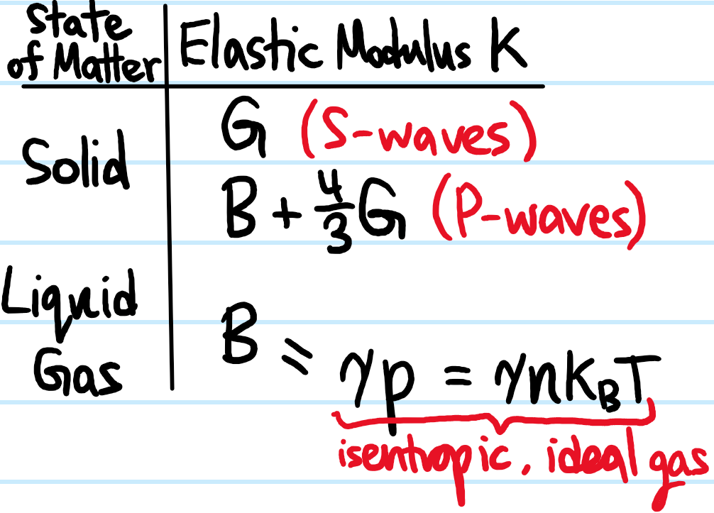
Problem: Define the specific acoustic impedance \(Z\) of a sound wave \(X(x,t)\) propagating in a non-dispersive medium (solid/liquid/gas) of density \(\rho\) with speed \(v\).
Solution: Similar to mechanical impedance except force is mapped to a pressure \(F\mapsto p\) to avoid dealing with the extensive nature of \(F\) depending on the area of application.
The pressure is \(p=-\rho c^2X’\) and the speed of the wave is \(\dot X\), so:
\[\dot X=\frac{-\rho c^2X’}{Z}\]
Either plug the travelling wave ansatz again \(X(x,t)=X(x-ct)\), or (equivalently) work in Fourier space:
To make it look more like the violin string, one can write:
\[c=\frac{\rho c^2}{Z}=\sqrt{\frac{K}{\rho}}\]
where \(K\) is a suitable elastic modulus that depends on the type of wave and medium:
Problem: Define the electromagnetic impedance \(Z\) of a propagating EM wave in some medium (free space, dielectric, conductor, etc.)
Solution: The general definition is:
\[H=\frac{E}{Z}\]
where of course \(E:=|\textbf E|\) and \(H:=|\textbf H\) are the orthogonal \(\textbf E\) and \(\textbf H\)-fields. Invoking the constitutive relation \(E=v\times \mu H\) in a linear dielectric gives:
\[Z=\sqrt{\frac{\mu}{\varepsilon}}\]
Of course this applies to a conductor where \(\varepsilon\mapsto\varepsilon_{\text{eff}}=\varepsilon+i\sigma/\omega\).
Problem: Define the electrical impedance \(Z\) of a lumped element in an electric circuit.
Solution: This is Ohm’s law:
\[I=\frac{V}{Z}\]
(the connection with waves is a bit hazy here?)
Problem: Define the characteristic impedance of a transmission line with inductance per unit length \(\hat L\) and capacitance per unit length \(\hat C\), series resistance per unit length \(\hat R\), and parallel conductance per unit length \(\hat G\).
In the lossless case \(\hat R=\hat G=0\), this simplifies to:
\[Z=\sqrt{\frac{\hat L}{\hat C}}\]
Problem: Now that the notion of an impedance has been defined for a bunch of scenarios,
Problem: Explain why, in all the cases considered, the notion of a wave impedance \(Z\)
Impedance helps with steady-state calculations, comes from a linear constitutive law/equation of state/is intrinsic to a medium.
Problem:
Solution: Don’t memorize:
\[r=\frac{Z-Z’}{Z+Z’}\]
\[t=\frac{2Z}{Z+Z’}\]
One option is to memorize directly the interface matching conditions:
\[1+r=t\]
\[Z-Zr=Z’t\]
they are logically equivalent, but the latter makes it clear where it comes from. Furthermore, multiplying the latter \(2\) equations together yields the power flow/energy conservation equation:
\[Z(1-r^2)=Z’t^2\]
ensuring that \(R:=r^2\) and \(T:=\frac{Z’}{Z}t^2\) obey \(R+T=1\).
Alternatively, in direct analogy with “conservation of momentum” and “conservation of kinetic energy” from the context of elastic collisions, one can also remember the pair of equations:
\[Z=Zr+Z’t\]
\[\frac{1}{2}Z=\frac{1}{2}Zr^2+\frac{1}{2}Z’t^2\]
and similarly, the equation \(v+v’=V\) from that context directly translates to the continuity condition \(1+r=t\).
Problem: Explain why in some contexts (notably optics) the impedance looks “swapped”
in other words, it would have been more natural to work with the admittances.
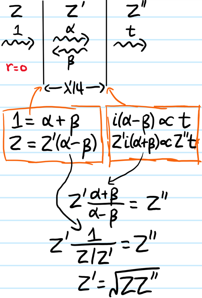
Problem: Impedance matching \(Z’=Z\) is desirable because it ensures that there are no reflections \(r=R=0\), i.e. perfect transmission \(t=T=1\). However, even if \(Z”\neq Z\), show that by inserting a length \(\lambda’/4\) of an intermediate medium with impedance \(Z’=\sqrt{ZZ”}\) the geometric mean, this acts to effectively impedance match anyways.
Solution: It is useful to first gain a heuristic understanding of this. Basically, the idea is that initially one has \(2\) media with mismatched impedances \(Z\neq Z^{\prime\prime}\); left like that, there would be reflections at the interface. So the idea is to insert an intermediate medium between the \(2\), where here the word “intermediate” not only means it’s literally intermediate between the \(2\) media, but also that its impedance \(Z’\) should be intermediate between the \(2\) (which will turn out to be the geometric mean). In other words, one is dealing with either a monotonically increasing or decreasing impedance “staircase”:
Then, when a wave is incident from the left, some of it will be reflected at the \(Z\neq Z’\) interface while some is transmitted. This transmitted light will then be incident on the \(Z’\neq Z^{\prime\prime}\) interface, and some of that will be reflected back towards the source, and get transmitted again through the original \(Z\neq Z’\) interface. Now, in order to eliminate any net back-reflection, one would like for \(2\) things to be true:
The \(2\) reflections should interfere destructively, i.e. be \(\pi\) out of phase.
Their amplitudes should also match up, so that one does indeed achieve complete destructive interference, rather than merely partial destructive interference.
Since there is a staircase setup, either both reflections got a \(\pi\)-phase shift or neither of them did. So in any case, this is basically nothing more than an application of thin film interference; the phase shift due to bouncing back and forth at normal incidence inside the intermediate medium of length \(L\) is:
with \(n=0\) being a common choice. As for the amplitude matching, unfortunately it doesn’t seem as straightforward to show that \(Z’=\sqrt{ZZ^{\prime\prime}\), since that does not imply:
(so it seems the tedious approach from matching boundary conditions is necessary? this is the quickest way I can think of for doing it with boundary conditions:)
Problem: Explain why megaphones are shaped like so:
Suppose you know that \(p\) is the derivative of some function with respect to \(v\). A natural question is whether or not the roles of \(v\) and \(p\) can be reversed, that is, can \(v\) also be viewed as the derivative of some (possibly different) function with respect to \(p\)? In symbols, if \(p=\frac{d\mathcal L}{dv}\) for some function \(\mathcal L\), then is there some (possibly different) function \(H\) such that \(v=\frac{dH}{dp}\)? The answer turns out to be yes, and moreover is unique modulo the addition of a constant. This function \(H\) is called the Legendre transform of \(\mathcal L\) from \(v\) to \(p\). It is a straightforward exercise in integration by parts to actually find an explicit formula for the Legendre transform \(H\) in terms of \(\mathcal L\), \(v\) and \(p\) by enforcing the “derivative symmetrizer” property described above:
$$v=\frac{dH}{dp}$$
$$dH=vdp$$
$$\int dH=\int vdp$$
$$H=vp-\int pdv$$
$$H=vp-\int\frac{d\mathcal L}{dv}dv$$
$$H=vp-\mathcal L$$
where in the last equation an arbitrary additive constant \(+C\) has been suppressed to zero as is conventional. Because of the derivative symmetrizer property, it is immediate that the Legendre transform of \(H\) from \(p\) back to \(v\) will just give \(\mathcal L\) again (i.e. the Legendre transform is an involution, or equivalently its inverse is equal to itself, hence as a corollary it preserves information).
In the context of classical mechanics, \(\mathcal L\) would represent the Lagrangian of a system while \(H\) would represent its Hamiltonian. The statement \(p=\frac{d\mathcal L}{dv}\) is then often viewed as the definition of the generalized momentum coordinate \(p\) conjugate to the generalized velocity coordinate \(v\) while the symmetric equation \(v=\frac{dH}{dp}\) often falls under the guise of one of Hamilton’s equations.
By contrast, in thermodynamics it is customary to use the Legendre transform with the opposite sign convention, so that instead of \(H=vp-\mathcal L\), it would be \(H=\mathcal L-vp\). This preserves the derivative \(p=\frac{d\mathcal L}{dv}\) (because \(H\) is not in that equation) but introduces a corresponding sign change in \(v=-\frac{dH}{dp}\) (because \(dH\mapsto -dH\)). For instance, starting from the combined first and second laws of thermodynamics:
$$dU=TdS-pdV+\mu_idN_i$$
One can Legendre transform \(U=U(S,V,N_i)\) along 3 distinct “axes”, namely \(S\to T, V\to -p\) or \(N_i\to\mu_i\), leading to three corresponding thermodynamic potentials:
The Helmholtz free energy \(F:=U-TS\)
The enthalpy \(H:=U+pV\)
The no-name thermodynamic potential \(?:=U-\mu_i N_i\)
From here, one can apply more Legendre transforms to change variables as much as one wants, noting that Legendre transforms commute. For instance, the Gibbs free energy \(G\) can be thought of as either the Legendre transform of the Helmholtz free energy \(F\) from \(V\to -p\) or as the Legendre transform of the enthalpy \(H\) from \(S\to T\):
$$G=F+pV=H-TS=U+pV-TS$$
Occasionally one also sees the grand thermodynamic potential \(\Phi:=F-\mu_iN_i\) defined as the Legendre transform of the Helmholtz free energy \(F\) from \(N_i\to\mu_i\) (this is also the Legendre transform of the earlier “no-name” thermodynamic potential \(?\) from \(S\to T\)).
Remember that fundamentally the Legendre transform is defined to be a derivative symmetrizer. This means for instance that because \(-p=\frac{\partial U}{\partial V}\) and the enthalpy \(H\) was the Legendre transform of \(U\) from \(V\to -p\), this means we get for free the symmetric derivative \(V=\frac{\partial(-H)}{\partial(-p)}=\frac{\partial H}{\partial p}\), and likewise for the others.
One final nota bene: often, it is said that the Legendre transform only exists for convex or concave functions \(\mathcal L\). This is because if the Legendre transform \(H=vp-\mathcal L\) is to be regarded as a function of \(p\), then one needs to be able to find a formula for \(v=v(p)=v\left(\frac{d\mathcal L}{dv}\right)\), but the only way one can actually have such a functional relationship is iff \(\mathcal L\) does not have the same derivative \(\frac{d\mathcal L}{dv}\) at distinct values of \(v\). In practice most functions one deals with in physics are convex/concave for instance a typical Lagrangian contains a kinetic energy term \(\mathcal L=\frac{1}{2}mv^2+…\) and quadratic parabolas \(v\mapsto\frac{1}{2}mv^2\) are a classic example of convex functions. When \(\mathcal L\) has inflection points with respect to \(v\), it may sometimes be possible to take a sort of piecewise Legendre transform. Alternatively, one can use the more general notion of the Legendre-Fenchel transformwhich works for all functions (even non-convex/non-concave functions) by simply defaulting to the \(v\in\textbf R\) which maximizes \(H=vp-\mathcal L\) if there are multiple \(v\) with the same \(p=\frac{d\mathcal L}{dv}\).
The purpose of this post is to explain where observables in non-relativistic quantum mechanics (notably the position \(\textbf X\), momentum \(\textbf P\), orbital angular momentum \(\textbf L\), spin angular momentum \(\textbf S\) and Hamiltonian \(H\) observables) arise from, and why they have the properties (e.g. commutation relations) that they do.
In one sentence, the answer is that they arise from smooth projective unitary Lie group representations on a quantum system’s state space \(\mathcal H\). Different quantum systems will live in different state spaces \(\mathcal H\) (e.g. a spinless quantum particle moving through space has \(\mathcal H\cong L^2(\textbf R^3\to\textbf C,d^3\textbf x)\), a qubit fixed in space has \(\mathcal H\cong \textbf C^2\), a spin-1/2 electron being deflected in the Stern-Gerlach experiment has \(\mathcal H\cong L^2(\textbf R^3\to\textbf C,d^3\textbf x)\otimes_{\textbf C}\textbf C^2\), etc.). Exactly what kind of state space \(\mathcal H\) the quantum system lives in determines what the measurable observables of that quantum system are (e.g. for the qubit with \(\mathcal H\cong \textbf C^2\), the only measurable observables are \(\textbf S\) and \(H\), meaning that \(\textbf X,\textbf P\) and \(\textbf L\) would all not be measurable observables. By contrast, for the spinless quantum particle moving through space with \(\mathcal H\cong L^2(\textbf R^3\to\textbf C,d^3\textbf x)\), the situation is almost the opposite, with \(\textbf X,\textbf P, \textbf L\) and \(H\) all measurable observables but not \(\textbf S\)). As an aside, this highlights why it is important to specify a priori what \(\mathcal H\) is for any given quantum system since that “sets the rules of the game” for what observables one can even sensibly talk about, let alone measure.
The key insight will be to understand and look at the derivative of a Lie group representation at the identity of the Lie group, since that’s also where the Lie algebra lives.
Definition: Let \(\phi^{\infty}:G\to GL(V)\) be asmoothrepresentation of a Lie group \(G\) on a vector space \(V\) (notation: the symbol \(\phi\) is meant to evoke that it’s a group homomorphism while the \(\infty\) superscript emphasizes that its smooth, i.e. that \(\phi^\infty\) is of class \(C^\infty\)). Then the derivative of \(\phi^\infty\) at the identity \(1\in G\) exists because \(\phi^\infty\) is assumed to be smooth, and is a map of Lie algebras \(\dot{\phi}^{\infty}_1:\frak g\to\frak{gl}\)\((V)\) defined for all “velocity vectors” \(\textbf V\in\frak g\) by:
The intuition is that the Lie group representation \(\phi^{\infty}\) is like a light source that projects the Lie group \(G\) down onto its shadow \(GL(V)\). The map \(t\mapsto e^{\textbf Vt}\) is then a trajectory (see one-parameter subgroup) of \(G\) which is depicted as a green bug walking around on \(G\) and passing through \(e^{\textbf 0}=1\) at time \(t=0\) with velocity vector \(\textbf V\). The shadow of this trajectory is drawn on \(GL(V)\). Thus, the derivative \(\dot{\phi}^{\infty}_1(\textbf V)\) is simply the velocity of the bug’s shadow (at the identity \(1\in GL(V)\)) as a function of the bug’s actual velocity \(\textbf V\) (at the identity \(1\in G\)), where the intuition is that the faster you move, the faster your shadow moves too.
There are some other names by which this “derivative of Lie group representation at the identity” \(\dot{\phi}^\infty_1\) is known. For instance, emphasizing the smooth manifold nature of the Lie groups \(G,GL(V)\), a differential geometer might call \(\dot{\phi}^\infty_1\) the pushforwardof \(\phi^\infty\) at the identity, viewing it as a generalized Jacobian, however we won’t pursue this terminology. \(\dot{\phi}^\infty_1\) is also called the induced Lie algebra representation (arising from \(G\)), and this terminology will be an essential way to think about it later, but for now it’s best to just think of it using the picture above.
Four important properties of \(\dot{\phi}^\infty_1\) are listed below with intuition, proofs, and examples:
Property #1: \(\phi^{\infty}\left(e^{\textbf V t}\right)=e^{\dot{\phi}^{\infty}_1(\textbf V)t}\) (i.e. this is just saying that \(\dot{\phi}^\infty_1(\textbf V)\) is indeed the shadow velocity at the identity).
Intuition/Proof: Don’t just look at the initial shadow velocity \(\dot{\phi}^{\infty}_1(\textbf V)\), instead look at the shadow velocity at all times \(t\in\textbf R\):
Expand \(e^{\textbf V(t+\Delta t)}=e^{\textbf V\Delta t}e^{\textbf Vt}\) (bug’s location on \(G\) at time \(t+\Delta t\) is just the location \(e^{\textbf Vt}\) at time \(t\) translated by the displacement \(e^{\textbf V\Delta t}\), or see BCH formula). Then write \(\phi^{\infty}(e^{\textbf V\Delta t}e^{\textbf Vt})=\phi^{\infty}\left(e^{\textbf V\Delta t}\right)\phi^{\infty}\left(e^{\textbf V t}\right)\) (bug’s shadow in \(GL(V)\) at time \(t+\Delta t\) is just the bug’s shadow \(\phi^{\infty}\left(e^{\textbf Vt}\right)\) at time \(t\) translated by the displacement’s shadow \(\phi^{\infty}\left(e^{\textbf V\Delta t}\right)\), or equivalently this is because \(\phi^{\infty}\) is a group homomorphism). Finally, factoring out the shadow’s location \(\phi^{\infty}\left(e^{\textbf Vt}\right)\) from the numerator and the limit gives a first-order ODE in the time domain:
which is solved (with the initial condition \(\phi^{\infty}(e^{\textbf 0})=\phi^{\infty}(1)=1\)) by \(\phi^{\infty}\left(e^{\textbf Vt}\right)=e^{t\dot{\phi}^{\infty}_1(\textbf V)}\).
Examples: The trivial representation \(\phi^\infty:G\to GL(\textbf C)\cong\textbf C-\{0\}\) of any group \(G\) defined by \(\phi^\infty(g):=1\) has derivative (at the identity) \(\dot\phi^\infty_1(\textbf V)=0\) and indeed \(e^0=1\). The defining representation \(\phi^\infty:SO(2)\to SO(2)\subseteq GL(\textbf R^2)\) of \(SO(2)\) on \(\textbf R^2\), defined by \(\phi^\infty(R):=R\) has derivative (at the identity) \(\dot\phi^\infty_1(\Omega)=\Omega\) and so of course \(\phi^\infty(e^\Omega)=e^\Omega\). The adjoint representation \(\text{Ad}:Sp(1)\to GL(\frak{sp}\)\((1))\) of the symplectic group \(Sp(1)\) of unit quaternions on its Lie algebra \(\frak{sp}\)\((1)\) of imaginary quaternions \(\text{Ad}_{\hat q}(\textbf x):=\hat q\textbf x\hat q^{-1}\) has derivative (at the identity) \(\dot{\text{Ad}}_1:=\text{ad}:\frak{sp}\)\((1)\to\frak{gl}(\frak{sp}\)\((1))\) defined by \(\text{ad}_{\textbf x}(\textbf r)=[\textbf x,\textbf r]\). And indeed this is just one version of the BCH formula: \(e^{\textbf x}\textbf re^{-\textbf x}=e^{[\textbf x,]}(\textbf r)=\textbf r+[\textbf x,\textbf r]+\frac{1}{2}[\textbf x,[\textbf x,\textbf r]]+\frac{1}{6}[\textbf x,[\textbf x,[\textbf x,\textbf r]]]+…\) (despite the temptation, note that \(e^{\text{ad}_{\textbf x}}(\textbf r)\neq e^{\text{ad}_{\textbf x}(\textbf r)}\)).
Property #2: \(\dot\phi^\infty_1(\text{Ad}_g(\textbf V))=\text{Ad}_{\phi^\infty(g)}(\dot\phi^\infty_1(\textbf V))\) for all \(g\in G,\textbf V\in\frak g\) (i.e. “tilting your head” \(\textbf V\mapsto \text{Ad}_g(\textbf V)\), then measuring the shadow velocity \(\dot\phi^\infty_1(\text{Ad}_g(\textbf V))\) is the same as measuring the “actual” shadow velocity \(\dot\phi^\infty_1(\textbf V)\), then tilting your head).
Intuition/Proof: This is just Property #1 but with \(\textbf V\mapsto \text{Ad}_g(\textbf V)\) (i.e. tilting your head into the basis of \(g\)).
The bug’s trajectory \(e^{\text{Ad}_g(\textbf V)t}\) in \(G\) is more simply \(\text{Ad}_g(e^{\textbf Vt})\) (because it’s fundamentally the same trajectory as \(e^{\textbf Vt}\) just viewed in the basis of \(g\). Another way of phrasing it is that \(\exp\) and \(\text{Ad}_g\) commute for all \(\textbf V\in\frak g\)). Then \(\phi^\infty(\text{Ad}_g(e^{\textbf Vt}))=\text{Ad}_{\phi^\infty(g)}(\phi^\infty(e^{\textbf Vt}))\) by homomorphism. Finally, applying Property #1 again re-expresses the actual shadow trajectory \(\phi^\infty(e^{\textbf Vt})\) as \(e^{\dot{\phi}^{\infty}_1(\textbf V)t}\). Thus, as it is we have two ways of expressing the shadow’s tilted trajectory. To get just the tilted initial shadow velocity, take \((\partial/\partial t)_{t=0}\) and the claim follows.
Example: In the case where \(\phi^\infty=\text{Ad}\) also happens to be the adjoint representation of \(G\), Property #2 leads to the curious identity \([g\textbf V g^{-1},\textbf W]=g[\textbf V,g^{-1}\textbf W g]g^{-1}\).
Property #3: \(\dot{\phi}^\infty_1(\alpha\textbf V)=\alpha\dot{\phi}^\infty_1(\textbf V)\) and \(\dot{\phi}^\infty_1(\textbf V+\textbf W)=\dot{\phi}^\infty_1(\textbf V)+\dot{\phi}^\infty_1(\textbf W)\) for all \(\alpha\in\textbf R, \textbf V,\textbf W\in\frak g\) (i.e. doubling the bug’s velocity doubles its shadow velocity and a vector addition of actual velocities corresponds to vector addition of shadow velocities).
Intuition/Proof: This is just the statement that \(\dot{\phi}^\infty_1\) is an \(\textbf R\)-linear transformation between vector spaces \(\frak g\)\(\to\text{gl}\)\((V)\). The scaling covariance is easy to check directly from the definition of the derivative. As for translational covariance, I haven’t been able to find any elementary way to do it, other than by appealing to various BCH-type formulas. The key obstacle is to get \(e^{\textbf V+\textbf W}\) to interact nicely with the homomorphism property of \(\phi^\infty\). One way is to apply the Zassenhaus formula:
in which one would freely interchange limits and derivatives, and apply the power rule.
Example: Taking again \(\phi^\infty=\text{Ad}\) as in the previous example, Property #3 simply says that the commutator looks like multiplication (or as mathematician’s prefer to say, bilinear).
Intuition/Proof: This is just Property #2 but with \(g=e^{\textbf Vt}\) and the \(\textbf V\) in Property #2 replaced by \(\textbf W\), then just take \((\partial/\partial t)_{t=0}\) and note that it commutes with \(\dot\phi^\infty_1\) because the latter is linear (Property #3). Essentially, there is a bug with velocity \(\textbf W\) at the identity \(1\in G\), and a second bug \(e^{\textbf Vt}\) that collides with the first bug at the identity at \(t=0\), and so \(\dot\phi^\infty_1(\text{ad}_{\textbf V}(\textbf W))\) should be read as “the shadow velocity of the first bug in the moving frame of the second bug when both collide at \(1\)”.
Example: Taking \(\phi^\infty=\text{Ad}\) again, one establishes the Jacobi identity \(\text{ad}_{\text{ad}_{\textbf V}(\textbf W)}(\textbf X)=\text{ad}_{\text{ad}_{\textbf V}}(\text{ad}_{\textbf W})(\textbf X)=\text{ad}_{\textbf V}(\text{ad}_{\textbf W}(\textbf X))-\text{ad}_{\textbf w}(\text{ad}_{\textbf v}(\textbf X))\), commonly written in the cyclic form \([\textbf V,[\textbf W,\textbf X]]+[\textbf W,[\textbf X,\textbf V]]+[\textbf X,[\textbf V,\textbf W]]=\textbf 0\). This corollary of Property #4 combined with the multiplicative nature of the commutator from Property #3 is actually a conceptually elegant way to prove that the tangent space \(\frak g\)\(=T_1G\) of any Lie group \(G\) at its identity is genuinely a (real) Lie algebra.
And because \(\frak g\) is a Lie algebra, Property #3 and Property #4 acquire a deeper interpretation; together, they assert that \(\dot\phi^\infty_1\) is a representation of the Lie algebra \(\frak g\) (on the same vector space \(V\)). Just as a representation of the Lie group \(G\) was a homomorphism from \(G\) to \(GL(V)\), a representation of a Lie algebra \(\frak g\) is a homomorphism from \(\frak g\) to \(\frak{gl}\)\((V)\). But for Lie algebras, the notion of “homomorphism” is different than for groups because they have different data/structures on them that require preserving (for Lie algebras, these are the real vector space structure and the Lie bracket whereas for groups it is just the composition of symmetries). Thus a Lie algebra representation is distinct from the concept of a group representation, but similar in spirit.
Thus, this explains the terminology “induced Lie algebra representation” from earlier. Abstractly, one can view differentiation of paths at the identity as a functor from the category of Lie group representations to the category of Lie algebra representations. It is natural to ask if such a functor is surjective, that is, if every Lie algebra representation arises in this way. For simply connected Lie groups \(G\), it turns out the answer is yes, but in general no (I’m not sure about the question of injectivity, but my intuition suggests it is injective between non-isomorphic Lie group representations due to Schur’s lemma).
Finally, we are in a position to explain where observables come from. The following concrete example illustrates this general procedure:
Example: Consider a spinless particle moving on the real line \(\textbf R\). It therefore has state space \(\mathcal H=L^2(\textbf R\to\textbf C,dx)\) with the usual protractor given in terms of position eigenbasis wavefunctions by \(\langle\psi_1|\psi_2\rangle:=\int_{-\infty}^\infty\overline{\langle x|\psi_1\rangle}\langle x|\psi_2\rangle dx\). One example of a smooth projective unitary representation \(\phi^\infty:G\to PU(\mathcal H)\) acting on \(\mathcal H=L^2(\textbf R\to\textbf C,dx)\) comes from the additive Lie group \(G=\textbf R\) via:
for some “translation” \(\Delta k\in\textbf R=G\) in de Broglie space (also called Fourier space, reciprocal space, dual space, momentum space, wave space, etc.). To wit:
\(\phi^\infty\) is indeed a representation of \(\textbf R\) because \(\phi^\infty_{\Delta k_1+\Delta k_2}=\phi^\infty_{\Delta k_1}\circ\phi^\infty_{\Delta k_2}\) (so it’s not merely a projective representation but an actual representation).
\(\phi^\infty\) is indeed unitary because \(e^{i\Delta kx}e^{-i\Delta kx}=1\) and an invariant integrand implies an invariant integral.
Now one would like to differentiate \(\phi^\infty\) at the identity \(1\in\textbf R\) to get the induced Lie algebra representation \(\dot{\phi}^\infty_1:\frak{R}\)\(\to\frak u\)\((L^2(\textbf R\to\textbf C,dx))/i\textbf R1\). The first thing is to figure out what the Lie algebra \(\frak R\) of \(\textbf R\) is. As one might intuitively expect, \(\frak R\)\(=\textbf R\) because the tangent line to \(1\in\textbf R\) is…well all of \(\textbf R\) (one way to argue this rigorously is to algebraically embed \(\textbf R\to SL_2(\textbf R)\) by viewing real numbers \(x\in\textbf R\) as the one-parameter subgroup of horizontal shearing matrices \(\begin{pmatrix}1 & x\\0 & 1\end{pmatrix}\in SL_2(\textbf R)\) and then noting that \(\frak{sl}\)\(_2(\textbf R)\cong\textbf R\)). Even though at the level of sets, \(\textbf R=\textbf R\) trivially, at the level of their structures it is important to emphasize that one of them \(\textbf R=G\) is first and foremost a (Lie) group whereas the other one \(\textbf R=\frak R\) is first and foremost a real vector space. The reason for emphasizing this is that it means the exponential map from the Lie algebra \(\textbf R\) to the Lie group \(\textbf R\) is not the standard real exponential that one is used to working with; instead, it is actually just the identity map \(e^x=x\). The reason for this is because the Lie group \(\textbf R\) is an additive group, not a multiplicative group (whereas matrix Lie groups are typically multiplicative, so for them the exponential map genuinely coincides with the matrix exponential). To see this rigorously, one has to look at the general definition of the exponential map in Lie theory in terms of a unique one-parameter subgroup and use the additivity (rather than multiplicativity) of the Lie group \(\textbf R\). All this is to say that:
where the reason for pushing forward \(1\in\textbf R\) in the Lie algebra is because it is the most natural basis vector \(\textbf R=\text{span}_{\textbf R}\{1\}\) for the Lie algebra (or a “generator for the Lie group \(\textbf R\)” as physicists say, where the phrase “generate” is synonymous with “exponentiates to (allowing arbitrary linear combinations of generators)”, i.e. the assumption is that the exponential is surjective, which will be true if \(G\) has a compact and connected topology). Of course, this is currently an anti-Hermitian linear operator, so the last step is to multiply by \(i\) to recover the position observable \(X\) in the \(x\)-direction:
A completely analogous procedure can be carried out with the SPUR \(\phi^\infty:\textbf R\to PU(L^2(\textbf R\to\textbf C,dx))\) defined by \(\langle x|\phi^\infty_{\Delta x}|\psi\rangle = \langle x-\Delta x|\psi\rangle\) (here the Lie group is also \(\textbf R\), but conceptually one thinks of it as the group of translations \(\Delta x\in\textbf R\) of real space rather than reciprocal space (or in the language of wave-particle duality, particle space rather than wave space). The induced Lie algebra representation pushed forward on the same generator \(1\) gives by the chain rule:
where we have set \(\hbar = 1\) in some suitable natural unit system. Finally, there is one more measurable observable associated to this 1D spinless quantum particle with \(\mathcal H=L^2(\textbf R\to\textbf C,dx)\). This time again it happens to be the Lie group \(\textbf R\) that acts on \(L^2(\textbf R\to\textbf C,dx)\) via the SPUR \(\phi^\infty_{\Delta t}|\psi(t)\rangle:=|\psi(t+\Delta t)\rangle\), but now \(\textbf R\) is to be thought of conceptually as the group of translations \(\Delta t\in\textbf R\) through time. Also interesting to note here is that we do \(+\Delta t\) rather than \(-\Delta t\) whereas for the spatial translations we had to do \(-\Delta x\) rather than \(+\Delta x\) (this reminds me of Minkowski’s metric tensor \(g=\text{diag}(1,-1,-1,-1)\) used to define the hyperbolic geometry of Minkowski spacetime in special relativity, though I’m not sure if there’s any connection there). Running the machine again gives (chain rule):
and multiplying by \(i\) gives the Hamiltonian observable \(H\):
$$H=i\frac{\partial}{\partial t}$$
which is of course also known as the (time-dependent) Schrodinger equation. By applying properties #1,#2,#3 and #4 of \(\dot{\phi}^\infty_1\) proved earlier, one can establish such facts as:
Unitary operators as Hilbert space homomorphisms? Also where does the role of irreducibility come in? I guess they literally are just a direct sum basis of all representations, so they are really the only interesting/fundamental ones.