and, for reasons that will become apparent soon, the electronic Hamiltonian \(\text H_{\text e}:=V_{\text{nn}}+T_{\text e}+V_{\text{ee}}+V_{\text{ne}}\) is thought of as consisting of the following terms:
For an arbitrary molecule, the corresponding molecular Hamiltonian \(H\) is difficult to diagonalize. Fortunately, the existence of large mass gap \(M_i/m_e\sim 10^3\) between the nuclei and electrons motivates the Born-Oppenheimer approximation. This consists of \(2\) steps:
Step #\(1\): Diagonalize the electronic Hamiltonian \(H_{\text e}\) by itself first, viewing the nuclei positions \(\{\textbf X_i\}\) as fixed parameters:
By adiabatically varying \(\{\textbf X_i\}\), one thereby obtains an effective potential energy surface \(E_{\text e}\{\textbf X_i\}\).
Step #\(2\): Solve \((T_{\text n}+E_{\text e}\{\textbf X_i\})|E\rangle=E|E\rangle\) to get the molecular energies \(E\).
in which the nuclei are taken to be roughly clamped \(T_{\text n}\approx 0\) about their equilibrium positions \(\langle{\textbf X}_i\) except that the internuclear potential:
permits small harmonic vibrations of the nuclei about their clamped equilibria, where \(\eta_i=X_i-\bar X_i\). By diagonalizing the Hessian \(\left(\frac{\partial^2 V_{\text{nn}}}{\partial X_i\partial X_j}\right)_{\text{eq}}\) in its eigenbasis of normal modes, one can obtain a set of fictitious nuclei whose vibrations are completely decoupled from each other, i.e. a bunch of independent harmonic oscillators.
Semiclassically, the perturbation due to an external electromagnetic wave \(\gamma\) is \(\Delta H_{\gamma}=-e\sum_{\text{electrons } i}\textbf E_0\cos(\textbf k\cdot\textbf x_i-\omega t)+e\sum_{\text{nuclei }i} Z_i\cos(\textbf k\cdot\textbf X_i-\omega t)\) where \(\omega=c|\textbf k|\).
In this interview, well-known theoretical physicist Frank Wilczek commented that “still to this day I think the quantum theory of angular momentum is one of the absolute pinnacles of human achievement. Just beautiful”. The purpose of this post is to give a flavor of why Wilczek might have thought that.
As (orbital/spin/total) angular momentum should be an observable, it therefore should arise from a smooth projective unitary representation \(\phi^{\infty}\) of some group acting on suitable state spaces \(\mathcal H\cong L^2(\textbf R^3\to\textbf C,d^3\textbf x)\). Unsurprisingly, that group is \(SO(3)\) with \(\phi^{\infty}:SO(3)\to PU(\mathcal H)\) being defined by \(\langle\textbf x|\phi^{\infty}_R|\psi\rangle:=\langle R^{-1}\textbf x|\psi\rangle\) where also \(R^{-1}=R^T\) (although it’s quite intuitive why it must be \(R^{-1}\) rather than \(R\), one can also check that only \(R^{-1}\) allows the homomorphism property \(\phi^\infty_{R_2R_1}=\phi^\infty_{R_2}\circ\phi^{\infty}_{R_1}\) to be satisfied). The induced Lie algebra representation is then \(\dot{\phi}^{\infty}_1:\frak{so}\)\((3)\to\frak u\)\((\mathcal H)/i\textbf R1\) given by \(\dot{\phi}^{\infty}_1(\tilde J)=\left(\frac{\partial}{\partial\theta}\right)_{\theta=0}\phi^{\infty}_{e^{\tilde{J}\theta}}\), so that one has the angular directional derivative:
Letting \(\tilde{J}_1,\tilde J_2,\tilde J_3\in\frak{so}\)\((3)\) be the standard generators of \(\frak{so}\)\((3)\) (i.e. \((\tilde J_i)_{jk}=\varepsilon_{ijk}\)). Consider substituting \(\tilde J:=\tilde J_3\) for instance. Then clearly, one has:
with \(\phi\) the usual cylindrical coordinate about the \(z\)-axis. It is instructive to prove this by writing \(\textbf x=\rho\hat{\boldsymbol{\rho}}_{\phi}+z\hat{\textbf k}\), \(\tilde J_3\textbf x=\hat{\textbf k}\times\textbf x\) and using the standard expression of the gradient in cylindrical coordinates \(\frac{\partial\langle\textbf x|\psi\rangle}{\partial\textbf x}=\frac{\partial\langle\textbf x|\psi\rangle}{\partial\rho}\hat{\boldsymbol{\rho}}_\phi+\frac{1}{\rho}\frac{\partial\langle\textbf x|\psi\rangle}{\partial\phi}\hat{\boldsymbol{\phi}}_{\phi}+\frac{\partial\langle\textbf x|\psi\rangle}{\partial z}\hat{\textbf k}\). Finally, to recover the angular momentum observables, one just does the usual multiply by \(i\hbar\), so for instance one has the familiar \(\langle\textbf x|L_3|\psi\rangle=-i\hbar\frac{\partial\langle\textbf x|\psi\rangle}{\partial\phi}\). This should be compared with formulas such as \(\langle\textbf x|\textbf P|\psi\rangle=-i\hbar\frac{\partial\langle\textbf x|\psi\rangle}{\partial\textbf x}\) and \(H|\psi\rangle=i\hbar\frac{\partial|\psi\rangle}{\partial t}\).
The commutation relations \([\tilde J_i,\tilde J_j]=\varepsilon_{ijk}\tilde J_k\) for \(\frak{so}\)\((3)\) are just an application of the Jacobi identity for \(\textbf R^3\) with the cross product \(\times\). It suffices to show \([\tilde J_1,\tilde J_2]=\tilde J_3\) for example. We have: \([\tilde J_1,\tilde J_2]\textbf x=\tilde J_1\tilde J_2\textbf x-\tilde J_2\tilde J_1\textbf x=\hat{\textbf i}\times(\hat{\textbf j}\times\textbf x)-\hat{\textbf j}\times(\hat{\textbf i}\times\textbf x)=(\hat{\textbf i}\times\hat{\textbf j})\times\textbf x=\hat{\textbf k}\times\textbf x=\tilde J_3\times\textbf x\). The commutator algebra for the angular momentum observables are then directly inherited from the commutation relations for \(\frak{so}\)\((3)\) thanks to the fact that \(\dot{\phi}^\infty_1\) is a Lie algebra representation. To wit, consider \([J_i,J_j]=[i\hbar\dot{\phi}^\infty_1(\tilde J_1),i\hbar\dot{\phi}^\infty_1(\tilde J_2)]=(i\hbar)^2[\dot{\phi}^\infty_1(\tilde J_1),\dot{\phi}^\infty_1(\tilde J_2)]=(i\hbar)^2\dot{\phi}^\infty_1([\tilde J_1,\tilde J_2])=(i\hbar)^2\dot{\phi}^\infty_1(\varepsilon_{ijk}\tilde J_k)=i\hbar\varepsilon_{ijk}J_k\). Or, on a more abstract level, it is clear that we have the isomorphism of Lie algebras \((\textbf R^3,\times)\cong(\frak{so}\)\((3),[,])\).
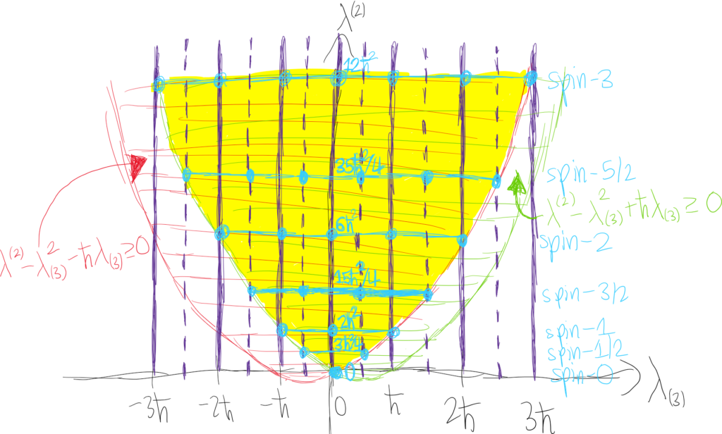
Anyways, armed with the commutator algebra \([J_i,J_j]=i\hbar\varepsilon_{ijk}J_k\), the spectrum \(\Lambda_{J_3}\) can be deduced. Letting \(\textbf J^2:=J_1^2+J_2^2+J_3^2\) be the Casimir invariant so that \([\textbf J^2,J_i]=0\), this means one can only know (i.e. measure with \(100\%\) certainty) the total angular momentum and angular momentum along one specific direction \(\hat{\textbf n}\). Arbitrarily orienting the coordinate axes so that \(\hat{\textbf n}:=\hat{\textbf k}\), this means the angular momentum \(J_3\) of the quantum particle along the \(z\)-axis is known and therefore is unknown in the \(xy\)-plane. Now, notice that \(\textbf J^2-J_3^2=J_1^2+J_2^2\). The right-hand side is a sum of squares, so there are two factorizations possible: \(J_1^2+J_2^2=(J_1+iJ_2)(J_1-iJ_2)+i[J_1,J_2]=(J_1-iJ_2)(J_1+iJ_2)+i[J_2,J_1]\). However, we’ve already worked out that \([J_1,J_2]=-[J_2,J_1]=i\hbar J_3\). Defining the mutually adjoint raising and lowering ladder operators \(J_{\pm}:=J_1\pm iJ_2\), this means that \(\textbf J^2-J_3^2+\hbar J_3=J_+J_-\) and \(\textbf J^2-J_3^2-\hbar J_3=J_-J_+\). In both cases, notice that both \(J_+J_-\) and \(J_-J_+\) are Hermitian and positive semi-definite (being of the standard SVD form, analogous to the number operator for the quantum harmonic oscillator). Thus, if \(|\lambda^{(2)},\lambda_{(3)}\rangle\) is a simultaneous eigenstate of \(\textbf J^2\) and \(J_3\) with the obvious eigenvalues, then the singular values must satisfy \(\lambda^{(2)}-\lambda_{(3)}^2+\hbar\lambda_{(3)}\geq 0\) and \(\lambda^{(2)}-\lambda_{(3)}^2-\hbar\lambda_{(3)}\geq 0\) (this has a nice geometric interpretation with two parabolas and the intersection in the middle region). The result is that for a given total angular momentum (squared) \(\lambda^{(2)}\), the angular momentum \(\lambda_{(3)}\) in the \(z\)-direction can only lie in an interval of width \(\sqrt{\hbar^2+4\lambda^{(2)}}-\hbar\) centered around \(\lambda_{(3)}=0\).
Now the part that I’m still figuring out how to understand deeply/motivate. Just as when one factorizes the Hamiltonian \(H_{\text{QHM}}\) of the quantum harmonic oscillator and realized that the factors turn out to act as raising and lowering operators for \(H_{\text{QHM}}\), so here the same phenomenon occurs. I feel that it depends not just on the fact that one is dealing with a sum of squares, but also works in both cases because the commutator is really simple. Once you know that, the proof is straightforward:
The intuition here is that it would be really nice if the \(J_3\) could act on the state instead since we know exactly what it will do \(J_3|\lambda^{(2)},\lambda_{(3)}\rangle=\lambda_{(3)}|\lambda^{(2)},\lambda_{(3)}\rangle\). So to be able to make this happen, the commutator emerges naturally as a necessity to compute, which fortunately we already know. This yields:
And by a similar computation, \(J_3J_-|\lambda^{(2)},\lambda_{(3)}\rangle=(\lambda_{(3)}-\hbar)J_-|\lambda^{(2)},\lambda_{(3)}\rangle\). Finally, since \([\textbf J^2,J_{\pm}]=0\) (as each of the \(J_i\) commute with \(\textbf J^2\)), this means that \(\textbf J^2J_{\pm}|\lambda^{(2)},\lambda_{(3)}\rangle=J_{\pm}\textbf J^2|\lambda^{(2)},\lambda_{(3)}\rangle=\lambda^{(2)}J_{\pm}|\lambda^{(2)},\lambda_{(3)}\rangle\). The key result is therefore that \(J_+\) and \(J_-\) can both be thought of as increasing or decreasing the total angular momentum of the system along the \(z\)-axis but without changing the total angular momentum \(\textbf J^2\). The mere existence of the ladder operators means ultimately that the end result is as depicted in the picture below. Read the vertical axis as imposing the total amount of angular momentum (squared) and the horizontal axis as imposing the amount of angular momentum in the \(z\)-direction, with the valid angular momentum eigenstates forming a hexagonal lattice of sorts.
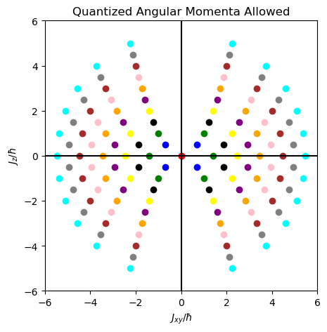
In physical space \(\textbf R^3\), the quantized angular momenta vectors allowed can be represented by this cross-section of the \(\rho\) vs. \(z\) plane. Below is for \(j=0,1/2,1,…,5\):
Focusing on the highest-weight states \(m_j=j\) (the inner parabolas in the diagram), for \(j=1/2\) the dark blue dots are inclined at the magic angle \(\theta_{1/2}=54.7^{\circ}\) from the \(z\)-axis, while for the \(j=1\) highest-weight states the angle is \(\theta_1=45^{\circ}\) as is intuitively clear from the plot. In general, it is straightforward to show that for that highest-weight state \(|j(j+1)\hbar ^2,j\hbar\rangle\), the angle decreases as \(\cos(\theta_j)=\sqrt{\frac{j}{j+1}}\) so that \(\lim_{j\to\infty}\theta_j=0\) (aside, one immediate conjecture is that there exists some relation between these angles \(\theta_j\) and the position representations \(\langle\textbf x|j(j+1)\hbar^2,j\hbar\rangle\) of these angular momentum eigenstates since the magic angle satisfies \(P_2(\cos(\theta_{1/2}))=0\) and if I remember correctly the angular momentum eigenstates are written in terms of spherical harmonics in the position representation which are defined via Legendre functions \(P_j^{m_j}(\cos(\theta))\) of the first kind…does it correspond to some kind of conical angular node?
If one wished, it is straightforward to compute the following explicit normalization constants (using the Condon-Shortley phase convention):
which will be real because \(-j\leq m_j\leq j\) as \(j\in\textbf N/2\) is by definition the highest weight (or spin) of the irreducible representation for which \(J_+|\lambda^{(2)},j\rangle=0\).
The Hamiltonian \(H_{RR}\) of a rigid rotor (rigid means no vibration, so one can safely set the potential energy \(V=0\)) consists entirely of rotational kinetic energy about its center of mass:
At this point, the spectrum \(\Lambda_{H_{\text{rigid rotor}}}\) of kinetic energies is easy to read off, where as usual \(j\in\textbf N/2\) and \(m_j\in\{-j,…,j\}\):
The ground state energy of the rigid rotor fixed in free space is thus \(E_{0,0}=0\) corresponding to no kinetic energy. In general, because \(I_3\ll I\), it follows that the lowest energy states should have \(m_j=0\) (i.e. no angular momentum about the \(z\)-axis so one can visualize how the rigid rotor necessarily ought to be spinning). This can only occur for integer total angular momenta \(j\in\textbf N\subseteq\textbf N/2\) where now:
\[E_{j,0}=j(j+1)\frac{\hbar^2}{2I}\]
Thus, the constraint \(j\in\textbf N\) means that if the rigid rotor is in state \(|j(j+1)\hbar^2,0\rangle\), then the smallest energetic transition it can make is by \(\Delta j=1\) and not \(\Delta j=1/2\) (EDIT: I’m so dumb bruh why was I even thinking this…clearly there ain’t such a thing as a “half-raising” or “half-lowering” operator). The smallest energy of the corresponding photon it can absorb/emit is (basically, recall that anytime one has a quadratic map \(j\mapsto j^2\) then the first differences \(\Delta j\propto j\)):
with angular frequency \(\omega^j_{j-1}=\Delta E^j_{j-1}/\hbar=j\hbar/I=j\omega^1_0\). If one models a carbon monoxide \(\text{CO}\) molecule as a rigid rotor in one of these low energy states, then about the center of mass one has \(I=\mu R^2\) where \(\mu=\frac{12\times 16}{12+16}\text{ u}\) is the reduced mass and \(R=112.8\text{ pm}\) is the bond length. These combine to yield a base photon frequency of \(f^1_0=\omega^1_0/2\pi=115.8\text{ GHz}\), which is close to the experimental \(f^1_0=113.17\text{ GHz}\), a very important spectral frequency in astronomy for the study of interstellar gas. One might inquire by what factor the angular velocity \(\Omega_j\) of the molecule’s rotation is related to the angular frequency \(\omega^j_{j-1}\) of photons absorbed/emitted. Since it was already mentioned that the rigid rotor in these low energy states does not rotate at all in the \(z\)-direction \(m_j=0\), it follows that \(|\textbf J|=I\Omega_j\), but we also know that \(|\textbf J|=\sqrt{j(j+1)}\hbar=j\hbar + O_{j\to\infty}(1)\) so \(\Omega_j\approx \omega^j_{j-1}\) as \(j\to\infty\) which is to be expected (e.g. from Maxwell’s equations applied to a rotating electric dipole), although if \(j\) gets too large then there may eventually be some \(m_j=\pm 1/2\) states popping up too?
The purpose of this post will be to review a standard method for passing from the classical to the quantum world (or more poetically, turning \(\hbar=0\) on to \(\hbar=1\) in natural units). This procedure is called canonical quantization.
It is first worth emphasizing a conceptual point. Morally, it is quantum mechanics, and not classical mechanics, that represents ground truth. Thus, the whole notion of trying to “pass” from the classical world to the quantum world (i.e. the whole notion of “quantizing” a classical theory) is a bit fallacious; from a logical perspective, it makes much more sense to start with quantum mechanics and pass the other way into the classical world by taking the limit \(\lim_{\hbar\to 0}\). For instance, the fact that a particle’s position and momentum along some direction \(\hat{\textbf n}\) can never be simultaneously known with certainty should be thought of as something very normal, the way things just are and have always been, and that one’s apparent ability to evade this principle in classical mechanics should be thought of as a strange, unusual luxury that deviates from the quantum norm. Although as classical creatures it is the Newtonian physics of the classical world that is certainly more intuitive, as a serious physicist it is essential to think clearly and get one’s priorities straight.
First Quantization (Nonrelativistic Quantum Mechanics)
Mathematically, canonical quantization \(f\mapsto\hat f\) is a Lie algebra representation that maps functions \(f\in C^{\infty}(\textbf R^2\to\textbf R)\) on classical phase space \(\textbf R^2\) to operators \(\hat f\in \frak u\)\((\mathcal H)\) on quantum state space \(\mathcal H\) (all this discussion is easily generalizable to a higher-dimensional phase space like \(\textbf R^{6N}\)). In the former, the Lie bracket is provided by the Poisson bracket \(\{,\}\) while in the latter the Lie bracket is the commutator \([,]\), and one requires canonical quantization to preserve this structure:
\[[\hat f,\hat g]=\widehat{\{f,g\}}\]
Thanks to Taylor’s theorem, a countably infinite basis of \(C^{\infty}(\textbf R^2\to\textbf R)\) is given by monomial functions on phase space of the form \((x,p)\mapsto 1,x,p,x^2,xp,p^2,…\), but it turns out there is good reason to stop at quadratic order. Specifically, it is worth noticing (using standard abuse of notation of writing e.g. \(x\) to mean the function \((x,p)\mapsto x\)) that the subspace \(\text{span}_{\textbf R}(1,x,p,x^2,xp,p^2)\subset C^{\infty}(\textbf R^2\to\textbf R)\) is in fact a \(6\)-dimensional Lie subalgebra of the Lie algebra \(C^{\infty}(\textbf R^2\to\textbf R)\):
In fact, the \(3\times 3\) yellow box highlighted above defines yet an even smaller Lie subalgebra \(\text{span}_{\textbf R}(1,x,p)\subset C^{\infty}(\textbf R^2\to\textbf R)\), called the Heisenberg Lie algebra. One can then check that the canonical quantization map, defined on the basis functions by:
\[\hat 1:=-i\hbar 1\]
\[\hat x:=-iX\]
\[\hat p:=-iP\]
\[\widehat{x^2}:=\frac{X^2}{i\hbar}\]
\[\widehat{xp}:=\frac{1}{i\hbar}\frac{XP+PX}{2}\]
\[\widehat{p^2}:=\frac{P^2}{i\hbar}\]
is a legitimate Lie algebra representation when restricted to either the first-order Heisenberg subalgebra \(\text{span}_{\textbf R}(1,x,p)\) or the quadratic subalgebra \(\text{span}_{\textbf R}(1,x,p,x^2,xp,p^2)\).
As an aside, the standard physicist’s convention with regards to the meaning of a Lie algebra representation is to instead impose the rule:
\[[\hat f,\hat g]=i\hbar\widehat{\{f,g\}}\]
with the extra factor of \(i\hbar\) compared with the mathematician’s convention. This makes it so that the canonical quantization map corresponds to “just putting hats on everything” (the exception is for the function \(xp\) below where a symmetric combination is used to maintain Hermiticity):
\[\hat 1:=1\]
\[\hat x:=X\]
\[\hat p:=P\]
\[\widehat{x^2}:=X^2\]
\[\widehat{xp}:=\frac{XP+PX}{2}\]
\[\widehat{p^2}:=P^2\]
Despite the hopes of Dirac and others that such a simple prescription could extend to a Lie algebra representation over all functions \(f\in C^{\infty}(\textbf R^2\to\textbf R)\) on phase space, it was subsequently shown in work of Groenewold and Van Hove that this is impossible; i.e. that there does not exist any “reasonable” quantization map that would continue to remain a Lie algebra representation beyond the subalgebra \(\text{span}_{\textbf R}(1,x,p,x^2,xp,p^2)\) of quadratic polynomials on phase space. One way to see this is that, continuing to cubic order, one could reasonably demand, in analogy to \(\widehat{xp}:=\frac{XP+PX}{2}\), that for instance \(\widehat{x^2p}:=\frac{X^2P+XPX+PX^2}{3}\).
But if this were so, then one can see that:
\[\{x^3,p^2\}=6x^2p\to 2i\hbar(X^2P+XPX+PX^2)\]
whereas, using (ironically) the identity \([f(X),P]=i\hbar f'(X)\) in light of the obvious analog \(\{f(x),p\}=f'(x)\):
So these disagree, at least if one were to implement canonical quantization using the Weyl transform as above (thus, this is not a rigorous proof that there isn’t some other clever way to quantize that preserves the Lie algebra structure consistently, but just an intuitive argument for why such a scheme can’t exist, and that at its heart the reason is due to the non-abelian nature of operators).
Second Quantization(Quantum Field Theory)
Just as one can implement canonical quantization to pass from classical particle mechanics on phase space to quantum particle mechanics on state space, one can perform an analogous procedure to pass from classical field theory to quantum field theory. More precisely, it will be most convenient to work in the framework of Hamiltonian classical field theory (if one were to start with Lagrangian classical field theory, then in lieu of canonical quantization one would instead utilize path integral quantization but fundamentally all of these are equivalent as they must be).
Recall that Lorentz invariance is often manifest in Lagrangian classical field theories because one can just check that all indices are suitably contracted in the theory’s Lagrangian density \(\mathcal L\) to check whether or not the theory’s action \(S=\int dtd^3\textbf x\mathcal L\) is Lorentz-invariant. By contrast, the Legendre transform to an equivalent Hamiltonian formulation of the same classical field theory doesn’t break Lorentz invariance, but obscures it, since defining the conjugate momentum field \(\pi^j(X):=\frac{\partial\mathcal L}{\partial\dot{\phi}_j}\) picks out a preferred time coordinate \(ct=x^0\) and this is further emphasized in the Hamiltonian density itself:
\[\mathcal H=\pi^i\dot{\phi}_i-\mathcal L\]
In the Schrodinger picture, a quantum field is considered to be an operator-valued function \(\phi(\textbf x)\) on space \(\textbf x\in\textbf R^3\) (not spacetime because in the Schrodinger picture one takes operators to be \(t\)-independent) which satisfies the canonical commutation relations (i.e. the commutation relations of the Heisenberg algebra that canonical quantization would aim to preserve):
In the Schrodinger picture, all the \(t\)-dependence lies in the state \(|\psi\rangle=|\psi(t)\rangle\) which evolves by the usual Schrodinger equation \(i\hbar\dot{|\psi\rangle}=H|\psi\rangle\) where \(H=\int d^3\textbf x\mathcal H\). However, note that \(|\psi\rangle\) is more like a “wavefunctional” than a “wavefunction” because it takes in some field \(\phi(\textbf x)\) as an input and outputs a complex number. Thus, to emphasize again, Lorentz invariance was already broken from the get-go, but here it’s just getting even worse since only space \(\textbf x\) appears in the field \(\phi(\textbf x)\) whereas only time \(t\) appears in the Schrodinger equation.
Depending on the nature of a particular chemical compound, there exist many experimental techniques for finding its molecular structure (David Tong would call these experimental techniques scattering which if one views light as a particle, would be an appropriate terminology). Examples include nuclear magnetic resonance (NMR) spectroscopy (where one also has the freedom to select any NMR-active nucleus with \(I\geq 1/2\) such as \(^1\text H\) or \(^{13}\text C\)), microwave spectroscopy, infrared (IR) spectroscopy, UV-visible spectroscopy, x-ray/electron/neutron diffraction, and mass spectrometry (with or without electrospray ionization). Notice that the spectroscopic methods are ordered in increasing energy \(E\) along the electromagnetic spectrum. Mass spectrometry is sort of an outlier in that it is not a spectroscopic method, but rather purely spectrometric. However, the spectroscopic methods are arguably the most important ones these days because they convey the richest amount of information, and several Nobel prizes in chemistry have basically gone to people who used these or similar techniques to determine the structures of very complicated (often biologically significant) molecules.
In NMR spectroscopy, the idea is to place a molecule in an external magnetic field \(\textbf B_{\text{ext}}\) (this is often actually the superposition of three magnetic fields, one uniform and constant, one uniform but oscillating, and one non-uniform but constant, details can be found here). Then, an NMR-active nucleus will have to first-order a Zeeman Hamiltonian of the form \(H_{\text{NMR-active nucleus}}=-\boldsymbol{\mu}\cdot\textbf B_{\text{ext}}\) where the nuclear magnetic dipole moment operator is \(\boldsymbol{\mu}=\gamma\textbf S\). Furthermore, define the dimensionless nuclear spin angular momentum operator \(\textbf I:=\textbf S/\hbar\) so that its spectrum is of the form \(\sqrt{I(I+1)}\) for \(I=0,1/2,1,3/2,…\). Thus, for both \(^1\text H\) and \(^{13}\text C\) nuclei which are NMR-active with \(I=1/2\), one has \(2I+1=2\) energy eigenstates (\(m_I=\pm 1/2\) or “spin-up” and “spin-down”) arising from Zeeman splitting, separated by \(\Delta E=\gamma\hbar|\textbf B_{\text{ext}}|\). However, this wouldn’t make NMR particularly useful as all identical nuclei would just experience the same \(\textbf B_{\text{ext}}\) and hence have identical energies and be indistinguishable. This is where two important perturbations are then added to the Hamiltonian \(H\) of the NMR-active nucleus. Specifically, one has \(H=H_{\text{Zeeman}}+H_{\text{screening}}+H_{\text{J-coupling}}\), where \(H_{\text{screening}}=-\boldsymbol{\mu}\cdot\delta\textbf B_{\text{ext}}\) with \(\delta\) the chemical shift tensor field and \(\delta\textbf B_{\text{ext}}\) thought of as the induced screening magnetic field at the NMR-active nucleus due to functional groups nearby (e.g. electronegative elements, diamagnetic shielding from \(e^-\) in an aromatic ring, forced hybridizations of valence atomic orbitals on the atom associated to that NMR-active nucleus, etc.). Meanwhile, \(H_{\text{J-coupling}}=\sum_{\text{all non-identical NMR-active nuclei } i}2\pi\hbar\textbf I\cdot(J\textbf I_i)\) where the sum runs over all NMR-active nuclei (or at least the ones close to the NMR-active nucleus of interest) including different elements (and excluding identical nuclei in identical magnetic environments). Here, \(J\) is the \(J\)-coupling tensor field, and this \(H_{\text{J-coupling}}\) interaction is mediated by the Fermi contact interaction, Pauli exclusion principle, and Hund’s rule. For viscinal \(^3J_{^1\text H-^1\text H}\) coupling of \(^1\text H\) nuclei, it is always possible to draw a Newman projection with an associated dihedral angle \(\theta\) between the two \(^1\text H\) nuclei, and the Karplus equation asserts that \(^3J_{^1\text H-^1\text H}(\theta)=f_2\cos(2\theta)+f_1\cos(\theta)+f_0\) for some empirical fitting parameters \(f_0,f_1,f_2\in\textbf R\). The intuition is thus that trans/anti protons \(\theta=180^{\circ}\) have the greatest viscinal coupling constant, followed by cis/eclipsed protons \(\theta=0\), and worst coupling is for orthogonal protons \(\theta=90^{\circ}\). There is pretty much an infinite rabbit hole of interactions that can arise with NMR spectroscopy (e.g. not just diamagnetic but also paramagnetic screening interactions in \(H_{\text{screening}}\), or interactions of the nuclear spin angular momentum with rotation of the molecule, or for NMR-active nuclei with \(I\geq 1\), a quadrupolar interaction? It’s a deep subject. Final comment: under isotropic motional averaging and within the secular approximation, one has \(\delta\mapsto\frac{1}{3}\text{Tr}(\delta)\) and likewise \(J\mapsto\frac{1}{3}\text{Tr}(J)\)and this is what is actually measurable and plotted on an NMR spectrum. Larger nuclear masses (e.g. \(^{13}\text{C}\)) will have larger chemical shift ranges.
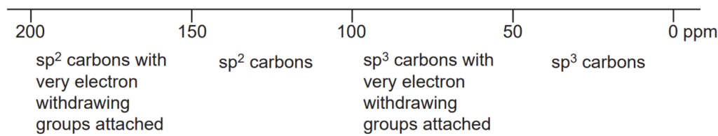
For \(^{13}\text C\) NMR spectroscopy:
Also, spin angular momentum coupling between \(^{13}\text C\) nuclei and \(^1\text H\) nuclei are typically suppressed via broadband proton decoupling. Also, due to low isotopic abundance, spin angular momentum coupling among \(^{13}\text C\) nuclei may only be visible as satellite peaks (unless the compound is \(^{13}\text C\)-enriched) and vice versa (i.e. in an \(^1\text H\)-NMR spectrum, the spin angular momentum coupling of protons with \(^{13}\text C\) nuclei would also only maybe appear as satellites). There is also a variant known as \(^{13}\text C\) attached proton test (APT) NMR spectroscopy which is essentially just the regular \(^{13}\text C\) NMR spectrum but it is also sensitive to the parity of the number of attached \(\text H\) atoms (look at which way the deuterated chloroform \(\text{CDCl}_3\) solvent points to determine this).
For \(^1\text{H}\)-NMR spectra \(n_{^1\text H}(\delta)\), the integral trace \(\int_{\delta_1}^{\delta_2}n_{^1\text H}(\delta)d\delta\) gives the number of protons with chemical shifts \(\delta\in[\delta_1,\delta_2]\). This is not the case for \(^{13}\text C\)-NMR spectra (why though?). Another quirk peculiar to \(^1\text{H}\)-NMR spectra is roofing (why does it happen?).
Exchangeable protons \(\text O-\text H\) and \(\text N-\textbf H\) can be made to disappear from a \(^1\text H\)-NMR spectrum using a \(\text D_2\text O\) shake (as \(\text H\to\text D\) which resonates at very different wavenumbers due to twice the nuclear mass).
In IR spectroscopy, no external field is needed. Just irradiate the sample with a bunch of infrared light and see if certain frequencies are absorbed more than others by the sample. These would correspond to normal mode/vibrational eigenstates of the molecule, which themselves tend to be dominated by particular functional groups. Although it’s really a quantum harmonic oscillator, one can think of a normal mode as a classical harmonic oscillator with \(\omega_0=\sqrt{\frac{k}{\mu}}\) where \(\mu=\frac{m_1m_2}{m_1+m_2}\) is the reduced mass (and as its name suggests, its generally closer to the smaller mass). An IR spectrum is then a plot of \(|\Delta\textbf p|(\nu)\), where \(\Delta\textbf p\) is the change in electric dipole moment associated with a given normal mode. Thus, purely covalent/non-polar bonds do not show up on IR spectra.
If one has a collection \(Q=\int\rho d^3x>0\) of positive charge \(\rho>0\) in some region of space, then the electric dipole moment \(\textbf p\) of \(Q\) may be viewed as \(\textbf p=Q\textbf X\), where \(\textbf X=\frac{1}{Q}\int\textbf x\rho d^3x\) is the center of charge in \(Q\) in direct analogy with the center of mass. On the other hand, for regions of negative charge \(\rho<0\), one can reflect the location of the charge across the origin and turn it into positive charge \(\rho(\textbf x)\mapsto-\rho(-\textbf x)\). Then one again recovers the center of charge interpretation of the electric dipole moment. Clearly, this operation (notably the reflection) in general depends on where one selects the origin to be. However, if the system of charges is neutral overall \(Q=0\), then the electric dipole moment \(\textbf p\) turns out to be origin independent. This \(Q=0\) neutral case is exemplified with the classic point electric dipole consisting of \(+q\) and \(-q\) charges separated by a displacement vector \(\Delta\textbf x\) pointing from \(-q\) to \(+q\). In this case, it is possible to convince oneself that it doesn’t matter where one places the origin, one always ends up with the result \(\textbf p=q\Delta\textbf x\). In this case, taking the dipole limit \(\lim_{q\to\infty,\Delta\textbf x\to\textbf 0,\textbf p=\text{constant}}\), one has the following equations governing how the dipole interacts with an external electric field \(\textbf E_{\text{ext}}\) (assuming \(\textbf B=\textbf 0\)). The external force is:
And the external electric potential energy relative to the configuration where the electric dipole is orthogonal to the external electric field \(\textbf p\cdot\textbf E_{\text{ext}}=0\) is then just (note the physical significance of the negative sign):
which satisfies \(\textbf F_{\text{ext}}=-\frac{\partial V_{\text{ext}}}{\partial\textbf x}\) thanks to standard vector calculus identities. Note also that \(\textbf E_{\text{ext}}\) in all these expressions is to be evaluated at the location \(\textbf x\) of the point electric dipole. Finally, note that in chemistry the electric dipole moment is defined in the opposite direction \(\textbf p_{\text{chemistry}}=-\textbf p\). For instance in a formula unit of \(\text{NaCl}\), the electric dipole moment \(\textbf p_{\text{chemistry}}\) would be considered to point from the \(\text{Na}^+\) cation to the \(\text{Cl}^-\) anion. This is because \(\textbf p_{\text{chemistry}}\) indicates the direction of greatest \(e^-\) density \(\rho_{e^-}<0\) which makes intuitive sense as electrons are the mobile charge carriers are in the case of \(\text{NaCl}\) they would be polarized towards the more electronegative \(\text{Cl}^-\). So ultimately this all goes back to Benjamin Franklin’s unwise choice of conventional current being the opposite of the actual direction of \(e^-\) flow.
Finally, a note that identical formulas hold for magnetic dipoles with \(\textbf p\mapsto\boldsymbol{\mu}\) and \(\textbf E_{\text{ext}}\mapsto\textbf B_{\text{ext}}\). Somewhat similarly to the electric dipole moment, the magnetic dipole moment is defined via \[\boldsymbol{\mu}:=\frac{1}{2}\iiint_{\textbf x\in\textbf R^3}\textbf x\times\textbf J(\textbf x)d^3x\].
Problem: Describe the wrong way to define a (Bravais) lattice.
Solution: A wrong way to define a Bravais lattice proceeds by \(3\) steps. First, one constructs the concept of a Delone set as any subset of a metric space with \(2\) properties:
(Uniformly Discrete) There exists a radius \(r>0\) such that one can “draw” \(r\)-balls centered at each point of the Delone set which are mutually disjoint.
(Relatively Dense) There exists a radius \(R<\infty\) such that one can “draw” \(R\)-balls centered at each point of the Delone set which cover the entire metric space.
For example, the discrete parabolic subset \(\{(n,n^2):n\in\mathbf Z\}\) of the metric space \(\mathbf R^2\) is not a Delone set because although one can take \(r:=1/\sqrt{2}\), there does not exist a finite radius \(R<\infty\) that makes the set relatively dense.
The next thing would then be to define a generic notion of “lattice” \(\Lambda\) as any Delone set in \(\mathbf R^d\) whose stabilizer subgroup \(\{\mathbf 0\}_{\Lambda}:=\{\mathbf x\in\mathbf R^d:\Lambda+\mathbf x=\Lambda\}\) of translational symmetries spans \(\text{span}_{\mathbf R}\{\mathbf 0\}_{\Lambda}=\mathbf R^d\).
Finally, one would qualify that one of these generic lattices \(\Lambda\) deserves to be called “Bravais” iff its stabilizer subgroup \(\{\mathbf 0\}_{\Lambda}\) acts transitively on \(\Lambda\).
The motivation for pursuing this approach is that one can then speak of “non-Bravais lattices” like the hexagonal honeycomb of graphene, as well as the aperiodic tilings in quasicrystals that count as Delone sets but would not be considered lattices.
Problem: Explain the simpler (and ultimately more useful) way to define a (Bravais) lattice.
Solution: The idea is to simply disqualify the hexagonal honeycomb of graphene from being a “lattice” despite how it may be referred to informally. Rather, one should view Bravais lattices as the fundamental objects, in which case a “lattice-like” object such as graphene would be considered the convolution of a triangular Bravais lattice with a \(2\)-carbon atom motif at each lattice point of the triangular Bravais lattice. Indeed, so fundamental are the Bravais lattices that henceforth they will simply be referred to (as is already standard practice in pure math) as lattices. Thus, a lattice \(\Lambda\) may be thought of in \(2\) logically equivalent ways:
i) There exist \(d\) linearly independent vectors \(\textbf x_1,\textbf x_2,…,\textbf x_d\in\textbf R^d\) such that \(\Lambda=\text{span}_{\textbf Z}(\textbf x_1,\textbf x_2,…,\textbf x_d)\) (such a \(\textbf Z\)-basis need notbe unique).
ii) Begin at any lattice point \(\textbf x\in\Lambda\), then close one’s eyes and walk to any other lattice point \(\textbf x’\in\Lambda\) without turning one’s head. After opening one’s eyes, it looks as if one hasn’t moved at all \(\textbf x’\cong\textbf x\).
For instance, the \(d=2\) triangular lattice is \(\textbf Z\)-spanned by the basis vectors \(\textbf x_1=a\hat{\textbf x}\) and \(\textbf x_2=\frac{a}{2}\hat{\textbf x}+\frac{\sqrt{3}a}{2}\hat{\textbf y}\).
Problem: Given a \(d\)-dimensional lattice \(\Lambda\) and a volume \(V\subseteq\textbf R^d\), what does it mean for \(V\) to be a cell of \(\Lambda\)?What does it mean if \(V\) is a primitive cell of \(\Lambda\)? What does it mean if \(V\) is a conventional cell of \(\Lambda\)? Give examples of \(d=3\) Bravais lattices \(\Lambda\) and cells thereof which are:
a) conventional but non-primitive
b) primitive but unconventional
c) primitive and conventional
d) non-primitive and unconventional
Solution: \(V\) is said to be a cell (commonly known by the misnomer “unit cell” which is a name that really should’ve been reserved for “primitive cell”) of \(\Lambda\) iff there exists a sublattice \(\Lambda’\subseteq\Lambda\) such that \(V+\Lambda’\) partitions \(\mathbf R^d\).
\(V\) is said to be primitive iff \(\Lambda’=\Lambda\), or equivalently iff each tessellate of \(V\) contains \(1\) lattice point so that in particular \(V\) occupies a volume \(|V|=|\det(\textbf x_1,\textbf x_2,…,\textbf x_d)|\) which is independent of the choice of basis \(\textbf x_1,\textbf x_2,…,\textbf x_d\).
By contrast, \(V\) is said to be conventional iff some crystallographer arbitrarily decided they like that cell \(V\) for \(\Lambda\) (typically because \(V\) is easier to visualize and/or more clearly highlights the point group symmetries of the lattice \(\Lambda\)). In particular, a conventional cell \(V\) may be (though not necessarily) non-primitive and thus may (though not necessarily) contain more than \(1\) lattice point.
a) For a face-centered cubic lattice \(\Lambda_{\text{FCC}}\), the cell \(V=[0,a)^3\) is the conventional, non-primitive cell of volume \(|V|=a^3\) containing \(N=4\) lattice points.
b) For \(\Lambda_{\text{FCC}}\), a primitive, unconventional cell \(V\) is the parallelepiped defined by the lattice vectors \(\Lambda_{\text{FCC}}=\text{span}_{\textbf Z}\left(\frac{a}{2}\hat{\textbf x}+\frac{a}{2}\hat{\textbf y},\frac{a}{2}\hat{\textbf x}+\frac{a}{2}\hat{\textbf z},\frac{a}{2}\hat{\textbf y}+\frac{a}{2}\hat{\textbf z}\right)\). It contains \(N=1\) lattice point and has volume \(|V|=a^3/4\).
c) For a primitive cubic lattice \(\Lambda_{\text{PC}}\), the cell \(V=[0,a)^3\) is both primitive and conventional containing \(N=1\) lattice point occupying a volume \(|V|=a^3\).
d) For \(\Lambda_{\text{PC}}\), the basis \(\Lambda_{\text{PC}}=\text{span}_{\mathbf Z}(a\hat{\mathbf x},a\hat{\mathbf x}+2a\hat{\mathbf y},a\hat{\mathbf z})\) defines a cell \(V\) that is both non-primitive (\(N=2,|V|=2a^3\)) and unconventional.
In what follows, it will be convenient to conflate the cell \(V\) and its volume \(|V|\), in particular writing both as just \(V\).
Problem: Define the reciprocal lattice \(\Lambda^*\) associated to a given real space lattice \(\Lambda\).
Solution: There are several logically equivalent formulations:
i) \[\textbf k\in\Lambda^*\Leftrightarrow\textbf k\cdot\textbf x\in 2\pi\mathbf Z\] for all \(\textbf x\in\Lambda\).
ii) If \(\textbf x_1,…,\textbf x_d\) is any \(\textbf Z\)-basis for \(\Lambda\), then the biorthogonal dual basis of \(d\) vectors \(\textbf k_1,…,\textbf k_d\) obeying \(\textbf k_i\cdot\textbf x_j=2\pi\delta_{ij}\) will be a \(\textbf Z\)-basis for \(\Lambda^*\).
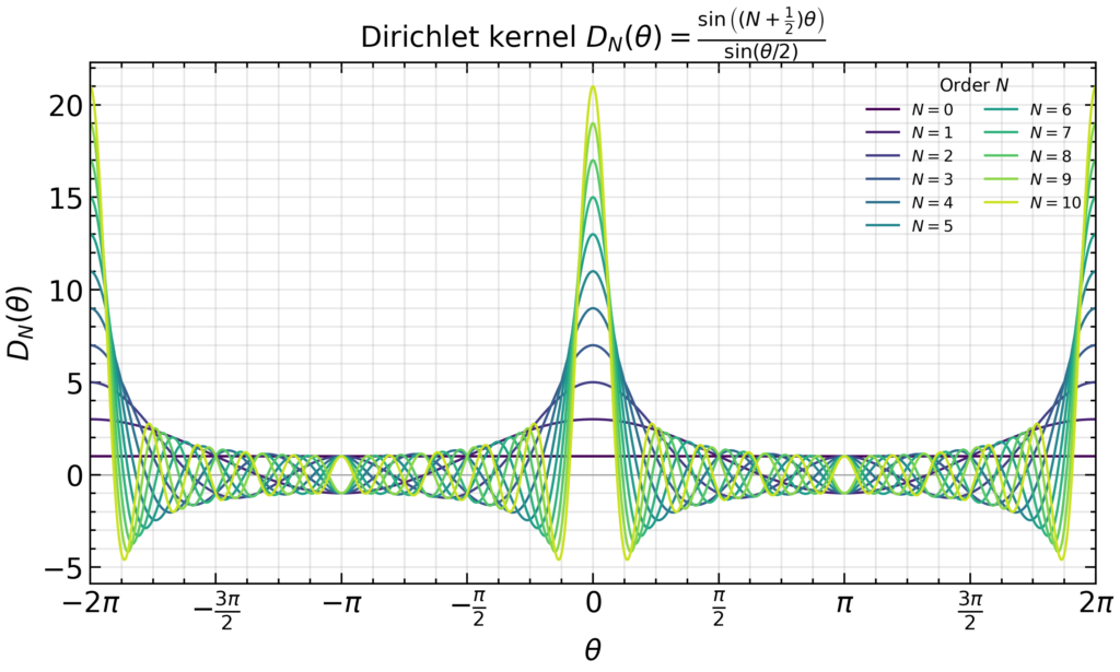
Furthermore, show that \(D_{\infty}(\theta):=\lim_{N\to\infty}D_N(\theta)=2\pi\sum_{n=-\infty}^{\infty}\delta(\theta-2\pi n)\) becomes the Dirac comb.
Solution: Since the Dirichlet kernel is just a geometric series with initial term \(e^{-iN\theta}\), common ratio \(e^{i\theta}\), and a total of \(2N+1\) terms:
So factoring out \(e^{i\theta/2}\) from the denominator, to expose \(-2i\sin\theta/2\) and hitting the numerator with it gives the result. For \(N=0,…,10\), the Dirichlet kernel is a \(2\pi\)-periodic function of \(\theta\) that peeks more and more strongly on \(D_N(\theta=2\pi n)=2N+1\) as \(N\to\infty\):
So it is intuitively clear that \(D_N(\theta)\propto\sum_{n=-\infty}^{\infty}\delta(\theta-2\pi n)\) will approach a Dirac comb as \(N\to\infty\), the only thing left is to compute the proportionality constant \(2\pi\). This follows either from the standard Dirichlet integral \(\int_{-\infty}^{\infty}dx\text{sinc}(x)=\pi\) (approximating the denominator \(\sin\theta/2\approx\theta/2\) for \(\theta\to 0\)) or reverting back to the exponential form \(\int_{-\pi}^{\pi}d\theta\sum_{n=-N}^Ne^{in\theta}=\int_{-\pi}^{\pi}d\theta e^{i0\theta}=2\pi\).
Problem: Let \(\Lambda\) be a lattice, let \(V\) be a primitive cell for \(\Lambda\), and let \(f(\mathbf x)\) be a \(\Lambda\)-periodic function. Define the structure factor \(f_V(\mathbf k)\) of \(f\) with respect to \(V\) and show that \(f(\mathbf x)\) has the Fourier series:
Solution: Since \(f(\mathbf x)\) is \(\Lambda\)-periodic, one can define a top-hat filtered \(f_V(\mathbf x):=f(\mathbf x)[\mathbf x\in V]\) with support only on the primitive cell \(V\), and hence (because \(V\) is primitive!) decompose:
as the convolution of \(f_V\) with a Dirac comb on \(\Lambda\). By the convolution theorem, the Fourier transform \(f(\mathbf k):=\int d^d\mathbf x e^{-i\mathbf k\cdot\mathbf x}f(\mathbf x)\) is given by:
where the structure factor is thus \(f_V(\mathbf k)=\int d^d\mathbf x e^{-i\mathbf k\cdot\mathbf x}f_V(\mathbf x)=\int_V d^d\mathbf x e^{-i\mathbf k\cdot\mathbf x}f(\mathbf x)\). Meanwhile, the “Laue kernel” may be expressed as a product of Dirichlet kernels:
In order for \(\prod_{i=1}^d\delta(\mathbf k\cdot\mathbf x_i-2\pi n_i)\neq 0\), one requires \(\mathbf k\cdot\mathbf x_i=2\pi n_i\) for all \(i=1,…,d\) so the Laue kernel is only non-vanishing for \(\mathbf k\in\Lambda^*\) and one may write:
where \(\mathbf k’:=n_1\mathbf k_1+…+n_d\mathbf k_d\in\Lambda^*\). The result then follows by writing \(\prod_{i=1}^d\delta((\mathbf k-\mathbf k’)\cdot\mathbf x_i)=\delta^d(X^T(\mathbf k-\mathbf k’))=\delta^d(\mathbf k-\mathbf k’)/|\det X|\), where the \(d\times d\) matrix \(X=(\mathbf x_1,…,\mathbf x_d)\) has determinant \(|\det X|=V\) so that \((2\pi)^d/V=V^*\).
The final upshot is that the inverse Fourier transform gives:
x-ray crystallography (in the Fraunhofer limit) is simply the art of photographing reciprocal space!)
Introduce the Wigner-Seitz primitive cell of a lattice; in reciprocal space called the Brillouin zone of \(\Lambda^*\), perpendicular bisector construction.
Problem: Although the Bravais lattices \(\Lambda\) considered so far have been, strictly speaking, infinite in extent, in practice all solids are finite in size, containing a finite number \(|\Lambda|<\infty\) of lattice points. Given this consideration, how many quantum \(\textbf k\)-states are available in each Brillouin zone (in the extended zone scheme; equivalently, in the reduced zone scheme this would be phrased as a question of how many \(\textbf k\)-states are available in each band).
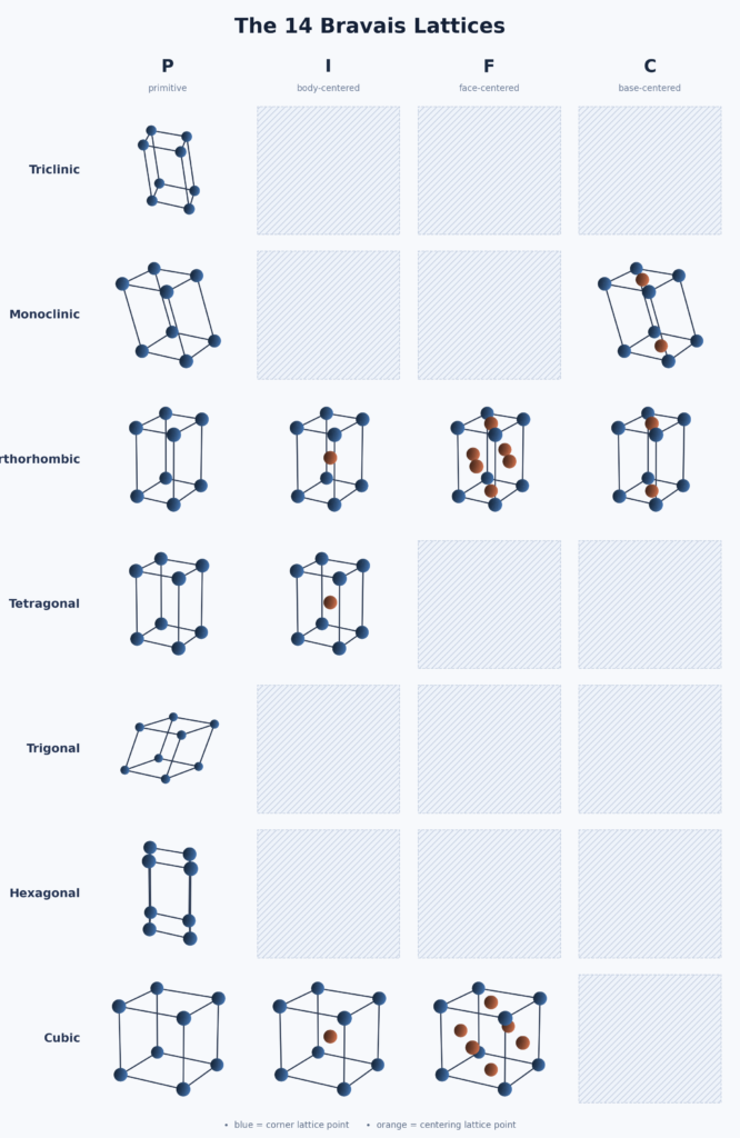
In \(\textbf R^3\), there is a standard classification of 3D Bravais lattices into \(14\) disjoint buckets based on how symmetric the conventional unit cell is (most symmetric is the primitive cubic 3D Bravais lattice, most asymmetric is the primitive triclinic 3D Bravais lattice, all the other 3D Bravais lattices lie on a spectrum somewhere in between).
A crystal \(\Gamma\) is the convolution of a 3D Bravais lattice \(\Lambda\) with a motif \(M\) of atoms or molecules: \(\Gamma=\Lambda*M\).
A lattice plane is any 2D affine subspace of the crystal \(\Gamma\), denoted by Miller indices \((hkl)\) where the reciprocal lattice vector \(h\textbf a^*+k\textbf b^*+l\textbf c^*\) is the normal vector the lattice plane. In other words, this yields the Weiss zone law \((U\textbf a+V\textbf b+W\textbf c)\cdot(h\textbf a^*+k\textbf b^*+l\textbf c^*)=hU+kV+lW=0\).
The multiplicity of a lattice plane \((hkl)\) is \(|\{hkl\}|\) and is at most \(|\{hkl\}|\leq 2^3\times 3!=48\).
There are \(2\) distinct solutions to achieving close packing of identical spheres in \(\textbf R^3\) (i.e. saturating the maximum packing efficiency of \(\eta=\frac{\pi}{3\sqrt{2}}\approx 74\%\)), namely the cubic close-packed crystal \(\Gamma_{\text{ccp}}\) and the hexagonal close-packed crystal \(\Gamma_{\text{hcp}}\) (this mathematical theorem is fundamentally why these two particular crystals are so important). Each of these crystals can be “deconvolved” into their conventional unit cell and motif \(\Gamma_{\text{ccp}}=\Lambda_{\text{fcc}}*\{(0,0,0)\}\) and \(\Gamma_{\text{hcp}}=\Lambda_{\text{ph}}*\{(0,0,0),(2/3,1/3,1/2)\}\).
Having said that both \(\Gamma_{\text{ccp}}\) and \(\Gamma_{\text{hcp}}\) are a close packing of identical spheres, they have associated close-packed
Both \(\Gamma_{\text{ccp}}\) and \(\Gamma_{\text{hcp}}\) also contain tetrahedral and octahedral interstices/voids which is typically where atoms/molecules of a second smaller element might go.
There are also several standard symmetries/point groups of 3D crystals \(\Gamma\): rotational symmetry (only \(4\) possible: diads, triads, tetrads, hexads due to the crystallographic restriction theorem), glide plane symmetry (glide planes not necessarily lattice planes), screw axis symmetry, and centrosymmetry \(\Gamma(-\textbf x)=\Gamma(\textbf x)\). Some of these are specific compositions of other symmetry elements.
Materials For Devices
Dielectric materials are electric insulators (\(\rho_f=0\)) and so are polarized by an external electric field \(\textbf E^{\text{ext}}\), leading to an induced polarization density \(\textbf P^{\text{ind}}=\varepsilon_0\chi_e\textbf E^{\text{ext}}\) reflecting the density of induced electric dipoles. Microscopic mechanisms of dielectric polarization are electronic polarization (any dielectric), ionic polarization (ionic crystals), and orientational polarization (e.g. water).
Centrosymmetric crystals \(\Gamma\) with \(\rho_b(-\textbf x)=\rho_b(\textbf x)\) are non-polar \(\textbf P=\textbf 0\).
Among non-centrosymmetric crystals, some are polar and some are non-polar.
Piezoelectric materials are dielectrics where application of an external stress \(\boldsymbol{\sigma}^{\text{ext}}\) leads to an induced polarization \(\textbf P^{\text{ind}}\), with constant of proportionality the piezoelectric coefficient \(\textbf P^{\text{ind}}=d\boldsymbol{\sigma}^{\text{ext}}\). This piezoelectric effect can also be run in reverse, whereby application of an external voltage \(V^{\text{ext}}\) leads to an induced strain \(\varepsilon^{\text{ind}}\) (not to be confused with the polarizability \(\varepsilon\)) where now \(\varepsilon^{\text{ind}}=V^{\text{ext}}\).
All polar materials are pyroelectric materials and vice versa (due to thermal expansion). This means an externally initiated temperature change \(\Delta T^{\text{ext}}\) induces a polarization \(\textbf P^{\text{ind}}\) via another proportionality constant called the pyroelectric coefficient \(|\textbf P^{\text{ind}}=p\Delta T^{\text{ext}}\) where \(p<0\).
Ferroelectrics are dielectrics exhibiting ferroelectrichysteresis (and hence have a spontaneous/remanent polarization \(\textbf P_0\) below their Curie temperature \(T_C\) (thus, any ferroelectric hysteresis loop should be viewed as a cross-section for some fixed temperature \(T<T_C\)).
Perovskites are crystals with stoichiometry \(\text{ABX}_3\) for \(\text{A,B}\) metal cations and \(\text X\) an anion. The Goldschmidt tolerance factor measures how distorted from a cubiccrystal structure the perovskite is, \(\Delta_{\text{cubic}}=\frac{R_A+R_X}{\sqrt{2}(R_B+R_X)}\).
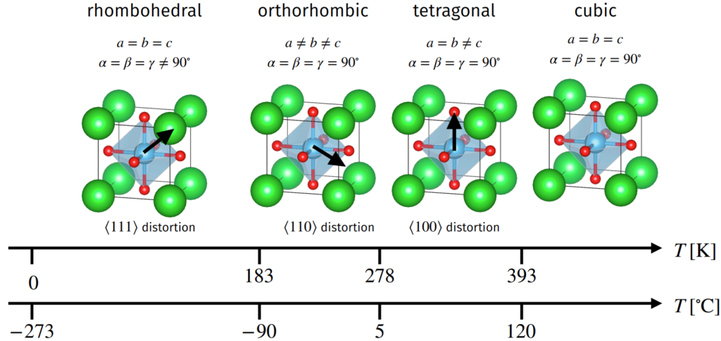
Barium titanate \(\text{BaTiO}_3\) is a ferroelectric perovskite with \(\Delta_{\text{cubic}}\approx 1.07\) so \(\text{Ba}^{2+}\) cations too large, lot of space for \(\text{Ti}^{4+}\) cation to polarize in the octahedral interstice. As a result, at temperatures \(T<T_C=120^{\circ}\text{C}\) such as room temperature \(T=20^{\circ}\text C\) it exhibits ferroelectric hysteresis. Specifically, cooling from \(T=T_C\), it undergoes a paraelectric-to-ferroelectric first-order phase transition in its 3D Bravais lattice \(\Lambda_{\text{pc}}\mapsto\Lambda_{\text{bct}}\) (and goes into other ferroelectric phases at lower temperatures still).
Landau theory can be used to explain semi-quantitatively the phenomenology of phase transitions. The idea is to postulate an ansatz for the Helmholtz free energy \(F:=U-TS\) and to then seek to minimize it (why not Gibbs free energy instead?) with respect to temperature \(T\) and an order parameter \(P\) (the induced polarization in this case).
Ferroelectrics are not necessarily monodomain (unless \(|\textbf E^{\text{ext}}|\) is sufficiently strong), but more commonly have many polarization domains separated by polarization domain walls due to an energetic competition between \(V_{\text{dipoles}}\) and \(V_{\text{stray}}\) (and it is the pinning of polarization domain walls by defects that gives rise to the irreversibility of ferroelectric hysteresis in the first place).
Ferroelectrics are useful for \(2\) main reasons: they have large polarizability \(\varepsilon\) so are used as dielectrics in capacitors, and because of their ferroelectric hysteresis properties for ferroelectric RAM, etc.
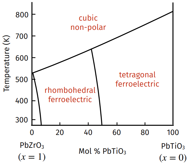
Another ferroelectric “perovskite” is lead zirconate titanate (PZT) \(\text{PbZr}_x\text{Ti}_{1-x}\text O_3\) where \(x\in[0,1]\), with the important composition being around \(x\approx 0.5\) at room temperature due to the presence of a morphotropic phase boundary there (the central \(\text{Ti}^{4+}\) cation can be polarized in a total of \(|\{100\}|+|\{110\}|=6+8=14\) distinct directions).
The magnetization field \(\textbf M:=n\boldsymbol{\mu}\) is the density of magnetic dipoles (analogous to the polarization density \(\textbf P:=n\textbf p\) as the density of electric dipoles).
Magnetic susceptibility is defined by \(\textbf M^{\text{ind}}=\chi_m\textbf H^{\text{ext}}\).
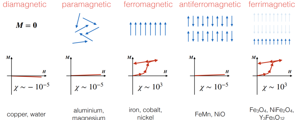
Using \(\textbf M\), magnetic properties of materials can be classified into \(5\) buckets: diamagnetic, paramagnetic, ferromagnetic, antiferromagnetic, and ferrimagnetic, where both ferromagnetic and ferrimagnetic materials have hysteresis loops:
For example, magnetite (where magnetism was discovered) is a ferrimagnetic material adopting an inverse spinel crystal structure.
Fundamentally, the origin of magnetism in matter is due to the exchange interaction energy and the Pauli exclusion principle (so parallel spins are energetically favorable to minimize exchange interaction energy, but this is in competition with thermal energy/entropic considerations that wants to randomize magnetic moments) hence existence of a Curie temperature \(T_C\) such that for \(T>T_C\), magnetization vanishes via a ferromagnetic-to-paramagnetic phase transition.
Ferromagnets have easy and hard axes due to magnetocrystalline anisotropy, and these easy and hard axes also give rise to shape anisotropy (e.g. explains why bar magnets and not “fat magnets”).
Ferromagnets exhibit magnetostriction.
For analogous energy competition reasons as ferroelectrics, ferromagnets also have magnetization domains separated by domain walls, and the reason for irreversible ferromagnetic hysteresis (domain wall pinning) is identical.
Ferromagnets subdivide into soft and hard ferromagnets, soft ferromagnets are important for transformers (need to be able to easily switch magnetization back and forth) whereas hard ferromagnets have microstructure engineered to deliberately pin domain wall motion (e.g. neodymium magnets).
Ionic conductors are described in the steady state by the Fick-Ohm-Boltzmann equation (called Nernst-Einstein equation for some reason) \(\frac{\sigma_{\infty}}{D_{\infty}}=\frac{nq^2}{kT}\).
Two important stochiometric defects are Schottky defects (simultaneous cation and anion vacancies) and Frenkel defects (an ion moves into an interstice, leaving behind a vacancy). The presence of such vacancies allows small ions to jump, mediating conduction. However, the jump is thermally activated (need enough thermal energy, described by Arrhenius equation \(D=D_0e^{-\Delta E_a/RT}\), so ionic conduction works best when served hot!
Doping zirconia (zirconium dioxide) \(\text{ZrO}_2\) with yttrium \(\text Y^{3+}\) cations forces creation of \(\text{O}^{2-}\) vacancies for charge neutrality. These vacancies mean that yttria-stabilized zirconia (YSZ) is an ionic conductor (called “stabilized” because the yttrium also stabilizes the otherwise unstable high-temperature cubic phase of zirconia).
Bismuth oxide \(\text{Bi}_2\text O_3\) in its cubic (\(\delta\)) phase is also an ionic conductor.
Ionic conductors are useful electrolytes in oxygen concentration cells for \(\lambda\)-sensors as vehicle exhaust control systems, and hydrogen fuel cells for the hydrogen economy.
Expected end-to-end distance in an \(N\)-monomer polymer chain is \(\sqrt{N}\ell_K\), where \(\ell_K\) is the Kuhn length of the polymer chain.
Polymers have an inherent anisotropy to them, this leads to their birefringence \(\Delta n:=n_{\text{slow}}-n_{\text{fast}}\) (and remember \(n=\sqrt{\hat{\mu}\hat{\varepsilon}}\)). Rotation angle of birefringence is \(\Delta\theta=k\Delta_{\gamma}x=2\pi\Delta n\Delta x/\lambda\). Typically studied under crossed polarizers, for white light source, the color blocked is complementary of color observed (as given on a Michel-Levy chart). For crossed polarizers, irradiance of all wavelengths also varies as \(\cos^2(\theta)\) (get extinction positions), enabling determination of fast and slow axes. To determine exactly which is which, use a compensator.
Polymers are examples of liquid crystals, formed at intermediate temperatures and classified by a unit director field \(\textbf D\) (don’t confuse with electric displacement field) and order parameter \(Q=\overline{P_2(\cos(\theta))}\) into nematic, smecticA/C, and chiral nematic (pitched/helical) liquid crystals. As with alignment of polarization domains in ferroelectrics or magnetization domains in ferromagnets, the same energy competition (alignment vs. thermal) drives the phase transitions (similarly get domain walls as seen in Schlieren textures, but these are now called disclinations where get Schlieren brushes). Unit director field \(\textbf D\) also defines slow and fast axes for birefringence of liquid crystals.
A chiral nematic liquid crystal can be enforced using Dirichlet boundary conditions on the unit director field \(\textbf D\), and an external \(\textbf E^{\text{ext}}\)-field can be applied to such a chiral nematic liquid crystal pixel to induce a Freedericksz ON/OFF phase transition, the key buzzword behind liquid crystal displays (LCDs).
Diffraction
X-rays are arguably the most important experimental tool in crystallography (and other fields of science such as chemistry and biology). The reason is that their wavelengths \(\lambda\sim 1 A\) just happens to coincide with the typical length scale of most of these crystal structures and molecules, etc. that one is interested in understanding the structure of so that they will indeed be resolvable. Typical source of x-rays include \(\text{Cu}\) \(K_{\alpha}\) with \(\bar{\lambda}\approx 1.542 A\).
For single crystals \(\Gamma\), the rule is that the lattice plane \((hkl)\) will usually diffract x-rays incident on the plane (in accordance with the Bragg equation \(\lambda=2d_{hkl}\sin(\theta_{hkl})\)) unless the structure factor \(\psi_{hkl}=0\) vanishes (in which case \((hkl)\) is said to be systematically absent, and different 3D Bravais lattices \(\Lambda\) have different selection rules about which lattice planes should or shouldn’t be systematically absent).
For polycrystals, typically have a powder of the polycrystalline material, hence called x-ray powder diffraction. Due to randomness of grain orientations, get both front and back reflections via Debye-Scherrer cones and irradiance \(I\propto |\{hkl\}||\psi_{hkl}|^2\) as in the Born rule. Can be imaged using a Debye-Scherrer camera on photographic film or using an electronic detector.
In general, any kind of photographic film or “sampling” of an interference pattern should be thought of as a slice through the reciprocal lattice \(\Lambda^*\) of the original 3D Bravais lattice \(\Lambda\). Bragg’s law has a nice interpretation in \(\Lambda^*\) via the Ewald sphere construction.
Transmission electron microscopy and scanning electron microscopy take advantage of the even finer de Broglie wavelength of electrons to image at even higher resolutions.
Microstructure
To image the microstructure of a material, can use reflected light microscopy (need a chemical etchant like Nital first to etch different phases at different rates), or for greater resolution, use SEM or atomic force microscopy (AFM).
Gibbs free energy \(G:=H-TS\) is minimized at constant \(p\) and \(T\). Thus, there is often an enthalpic (\(H\)) and entropic (\(-TS\)) competition that determines the equilibrium phases of a material at given conditions, with the general theme being that in the hot limit \(T\to\infty\), entropic effects dominate whereas in the cold limit \(T\to 0\) enthalpic effects dominate.
Since \(dG=Vdp-SdT\), it follows that the slope \(\left(\frac{\partial G}{\partial T}\right)_p=-S<0\) is always negative. For two phases, the temperature \(T_{12}\) at which \(G_1=G_2\) is the phase transition temperature between those phases (although this is for equilibrium only; phase diagrams only show equilibrium phases of globally minimum \(G\), but metastable phases of locally minimum \(G\) can persist if there is sufficient activation energy barrier).
For any solution of two atomic species \(A,B\), the Gibbs free energy of mixing is \(\Delta G_{\text{mix}}=\Delta H_{\text{mix}}-T\Delta S_{\text{mix}}\). Assuming only nearest-neighbor interactions matter, then \(\Delta H_{\text{mix}}=H_{\text{sol}}-H_{\text{mech mix}}=\lambda_{AB}x_Ax_B\) where \(x_A=n_A/n,x_B=n_B/n\) are mole fractions and \(\lambda_{AB}\sim nC(2H_{AB}-H_{AA}-H_{BB})\) is the \(AB\)-interaction parameter and \(C\) is a coordination number. Meanwhile, ignoring thermal contributions to entropy, \(\Delta S_{\text{mix}}=S_{\text{sol}}-S_{\text{mech mix}}=-nR(x_A\ln(x_A)+x_B\ln(x_B))\) is just a linear combination. The solution is ideal iff \(\Delta H_{\text{mix}}=\lambda_{AB}=0\) (meaning that \(A\) and \(B\) are probably quite similar) and regular otherwise. Thus, the regular solution model “Lagrangian” is: $$\Delta G_{\text{mix}}=\lambda_{AB}x_Ax_B+nRT(x_A\ln(x_A)+x_B\ln(x_B))$$
If \(\lambda_{AB}\leq 0\), then \(\Delta G_{\text{mix}}<0\) always, and
The more interesting case is \(\lambda_{AB}>0\) since then at low \(T\) the enthalpic term dominates and segregation of phases occurs whereas at high \(T\) the entropic term dominates again and get a uniform solution once more.
Regular solution model is only an approximation, has many assumptions built into it.
In practice, determine compositions by using a phase diagram and proportions using tie lines and lever rule.
Eutectic phase transitions are of the form \(L\to\alpha+\beta\), and generally have a lamellar microstructure/intergrowth due to cooperative diffusive growth. Are important in solder, where a low melting point is desirable (melting point of eutectic alloy of solder is lower than either of the pure metals).
Experimentally, phase diagrams can be mapped out by measuring cooling curves \(T(t)\) for a given composition of two atomic species. Changes in the cooling rate \(\dot T\) suggest phase transitions, and \(\dot T=0\) is a hallmark of eutectic solidification \(L\to\alpha+\beta\).
Rapid/non-equilibrium solidification leads to coring of the solid that is solidified. Such solids may also be dendritic in nature.
So far have just considered thermodynamics, need consider kinetics too. Homogeneous nucleation of a solid phase \(\alpha\) in a liquid \(L\) (both of the same composition), the driving force \(\Delta G_V\) for a supercooling of \(\Delta T<0\) is \(\Delta G_V=\Delta T\Delta S_V\) (assuming the heat capacity \(C_p\) is independent of \(T\)), and so spherical nucleation is governed by a “Lagrangian” \(\Delta G(r)=\frac{4}{3}\pi r^3\Delta G_V+4\pi r^2\gamma\) with the work of nucleation being \(\Delta G^*=16\pi\gamma^3/(3\Delta G_V^2)\) (note the essential proportionalities) and \(r^*=-2\gamma/\Delta G_V\) (again, the proportionalities should make sense).
Nucleation rate (nucleations per unit volume per unit time) varies with temperature \(T\) as: \(\dot{N}(T)\propto N_Se^{-\Delta G^*(T)/RT}e^{-E_a/RT}\), where the notation \(\Delta G^*(T)\) emphasizes that the driving force also depends on \(T\) via the supercooling \(\Delta T=T-T_m\).
When a solid phase \(\alpha\) nucleates inside another solid phase \(\beta\) (not liquid), no longer a sphere (as it was for a liquid), instead need consider coherency of interfaces. Incoherent interfaces have high surface energy \(V_{\gamma}\propto\gamma\), so tend to try and minimize incoherent surface area and therefore (counterintuitively) want to grow in the direction of incoherent interfaces.
\(\Gamma_{\text{Widmanstatten}}\) is a crystal structure found in certain \(\text{Fe}\)-\(\text{Ni}\) meteorites with sufficiently slow cooling rate \(\dot T\), shows how \(\Lambda_{bcc}\) and \(\Lambda_{fcc}\) iron-rich phases can have coherent interface.
Isothermal Transformation (TTT) Diagrams are for a fixed composition.
Displacive phase transitions (e.g. austenitic fcc steel undergoing a martensitic bct phase transition) are in contrast to reconstructive phase transitions.
The standard phase diagram for the \(\text{Fe}\)-\(\text{C}\) alloy system is actually only a quasi-equilibrium phase diagram. Cast irons have \(2%<w_{\text{C}}<4\%\) whereas steels have \(0.1%<w_{\text{C}}<1.5\%\) and the latter are dominated by a eutectoid phase transition to form pearlite = ferrite + cementite.
With steels however, there is a lot of metallurgical wisdom that has been gathered over the years on ways to manipulate the steel to get more properties out of it.
To harden a steel, the standard 3-step recipe is: anneal, quench, temper. First, anneal the steel up into the austenitic \(\gamma\) phase and wait until it equilibrates. Then quench it rapidly in water. This prevents the interstitial carbon \(\text C\) atoms from diffusing to form the lamellar eutectoid microstructure and instead results in them occupying octahedral interstices in a bct \(\text{Fe}\) matrix. This \(\Lambda_{\text{bct}}\) is thus considerably strained, impeding dislocation motion (so hard) but also brittle. To reduce brittleness while maintaining hardness, tempering is used (hold at some sub-eutectoid \(T\)) to introduce small cementite precipitates in ferrite matrix (very different from how it would look for eutectoid phase transition).
Al-Cu alloy system is important in aerospace engineering applications.
In general, strength \(\sigma_y\) increases with smaller grains \(d\) via the Hall-Petch equation \(\sigma_y=\sigma_0+k/\sqrt{d}\) (grains impede dislocation glide), hence the fuss about finer microstructure.
Al-Cu alloys undergo the same 3-step processing to harden them: anneal, quench, temper. In this third tempering step, the incoherent tetragonal structure of the \(\theta\) phase means that several intermediate metastable phases form first: GP zones, \(\theta”\), \(\theta’\) and finally \(\theta\), becoming more and more incoherent.
Mechanical Behavior of Materials
For uniaxial loading along some lattice direction in a crystal, can experimentally measure a stress-strain curve or \(\sigma^{\text{ext}}\)-\(\varepsilon^{\text{ind}}\) curve. In fact, in the elastic deformation regime defined by small external stress \(\sigma^{\text{ext}}\), the strain increases linearly in accordance with Hooke’s law \(\varepsilon^{\text{ind}}=\frac{\sigma^{\text{ext}}}{E}\) where \(E\) is Young’s modulus. Atomic origin of this linearity can be attributed to quadratic nature of Lennard-Jones potential energy at the equilibrium distance \(r_0\), and pursuing this line of reasoning fully, one even estimates \(E\sim\frac{1}{r_0}\frac{d^2V}{dr^2}(r_0)\) so that sharper potential wells and closer-packed lattice planes mean stiffer materials.
Beyond the yield stress \(\sigma^{\text{ext}}_y\), materials undergo irreversible plastic deformation (cf. so many of the other irreversible phenomena in this course notably ferroelectric and ferromagnetic hysteresis). Fundamental insight is that the origin of such plastic deformation turns out to be due to dislocation glide on close-packed lattice planes and in close-packed lattice directions in crystals, providing low-energy-cost way for whole a** lattice planes to effectively glide and thereby leading to plastic deformation.
Poisson’s ratio is roughly speaking \(\nu:=-\frac{\varepsilon_{\rho}^{\text{ind}}}{\varepsilon_{z}^{\text{ext}}}\) in the limit of small external strains (really external stresses). Metals usually have \(\nu\approx 0.3\), and \(nu=0.5\) is the condition for incompressibility (e.g. rubbers).
Ductility is measured by the failure strain \(\varepsilon_f\). Ductile materials have large \(\varepsilon_f\) whereas brittle materials have low \(\varepsilon_f\).
Analogous relation for shear stresses and their induced shear strains: \(\gamma^{\text{ind}}=\frac{\tau^{\text{ext}}}{G}\) where \(G\) is the shear modulus.
Note that \(E=2G(1+\nu)\) so the \(3\) are not independent of each other.
Total strain energy density is \(u=\frac{1}{2}E\varepsilon^2+\frac{1}{2}G\gamma^2\).
In many materials, Young’s modulus \(E\) (and I would imagine shear modulus \(G\)) is a tensor field due to anisotropy, for instance in fiber composites. Can use the Voigt or Reuss models to estimate the Young’s moduli parallel and perpendicular to the fibers based on volume fractions of fiber and matrix (although not super accurate).
Phenomenon of thermal expansion (and its linear nature over most temperature ranges) can be rationalized via the asymmetry of the LJ potential (think of as a ball rolling back and forth down the potential well). Leads to thermal stresses in bimetallic strips and any interface of two different metals joined together.
Euler-Bernoulli beam theory.
Important: Experimentally, plastically deformed materials appeared to have parallel stripes on their surfaces when loaded axially \(\sigma^{\text{ext}}\).
Closer examination showed that each stripe was like a little stair on a staircase (will turn out to be of magnitude \(|\textbf b|\)); lattice planes of that specific orientation had seemed to glide ever so slightly, and this was what caused the plastic deformation. But if one naively adapts a block-slip model of calculating the critical shear stress \(\tau^*\) needed to move a lattice plane over another lattice plane, one obtains values that far exceed experimental observations. Turns out there is a loophole, a way to make it seem as if an entire lattice plane had slid across another one, but requiring far less stress (Peierls-Nabarro stress \(\sim Ge^{-2\pi w/|\textbf b|}\)). Dislocations (ruck through carpet analogy)! Most materials contain dislocations (and indeed, very pure materials with no dislocations can approach the block-slip \(\tau^*\)).
Dislocations \(:=\) 1D (line) defects (cf. vacancies as 0D defects, cracks as 2D defects?). Thus, dislocations are a subset of defects.
Edge dislocations have line vector \(\boldsymbol{\ell}\) along the bottom of the extra half-plane of atoms, and Burgers vector \(\textbf b\in\Lambda\) orthogonal to it (complete the Burgers circuit).
Also have screw dislocations where \(\boldsymbol{\ell}\) is along the helical “screw axis” and Burgers vector \(\textbf b\) now parallel to \(\boldsymbol{\ell}\) by the magnitude of the dislocation.
Most dislocations have both edge character and screw character (cf. hybrid atomic orbitals having \(s\) character and \(p\) character). However all dislocations, regardless of their exact edge/screw character give the same net effect of making lattice planes glide (ruck in the carpet again!) and glide on the glide plane \(\text{span}_{\textbf R}(\textbf b,\textbf{\ell})\) provided there is sufficient shear stress (much less than the block-slip model, but still non-zero as determined by projecting the external tensile stress \(\sigma^{\text{ext}}\) onto the lattice plane to obtain a resolved shear stress \(\tau^{\text{ind}}=\sigma^{\text{ext}}\cos(\phi)\cos(\lambda)\)). Note that \(\lambda\) and \(\phi\) are not in general complementary angles, rather I believe \(90^{\circ}\leq\lambda+\phi\leq 180^{\circ}\).
Dislocation loops can either be vacancy loops or interstitial loops.
A dislocation can be thought of as having a free body diagram consisting of a fictitious “glide force” (not fictitious in the sense of non-inertial but just actually fictitious because dislocations are not actual objects) and some resistive drag force. The glide force \(\textbf f\) is a force per unit length (makes sense, dislocations are 1D defects) and is \(\textbf f=\tau^{\text{ind}}\textbf b\).
Shear strain energy (per unit line vector length) stored in a screw dislocation is \(V\approx \frac{1}{2}G|\textbf b|^2\). Edge dislocations have similar formula, and are more energetically costly than screw dislocations (per unit length).
For a given stress \(\boldsymbol{\sigma}^{\text{ext}}\), the close-packed slip system to activate first will have the largest Schmid factor (i.e. closest to \(\cos^(45^{\circ})=1/2\)). For crystals \(\Gamma\) admitting \(\Lambda_{\text{bcc}}\) or \(\Lambda_{\text{fcc}}\) 3D Bravais lattices, these are given conveniently by the OILS rule (why does it work?).
During loading, the slip direction rotates towards the tensile axis \(\lambda\to 0\).
From the frame of the sample however, one can think of the tensile axis rotating towards the slip direction instead, and this is made explicit by adding multiples of the slip direction to the tensile axis until two of the indices of the rotated tensile axis have same components (at which point duplex slip is initiated on the two lattice planes with equal Schmid factor), and the tensile axis starts rotating toward the sum of their slip directions. Since number of lattice planes and interplanar spacing is assumed conserved during plastic deformation, it follows that one has the Heisenberg quantities \(L\cos(\lambda)=\text{constant}\) and therefore by complementarity \(L\sin(\phi)=\text{constant}\) (just think intuitively about these are referring to!).
Basically, to explain plastic deformation to a 5-year old, put your hands (lattice planes) together and show one “crawling” over the other (dislocation propagating like ruck in carpet).
For \(\Gamma_{\text{hcp}}\), there may be geometric softening in the plastic deformation regime.
For \(\Gamma_{\text{fcc}}\), there are \(3\) stages of plastic deformation: constant \(\sigma\) (easy glide), followed by work hardening, followed by cross slip (occurs earlier for higher stacking fault energies because partial dislocations are less separated and need to combine since they are not pure screw character). In polycrystals, the average Schmid factor is called the Taylor factor, and is \(\overline{\cos(\phi)\cos(\lambda)}=\frac{1}{3}\) but this does not yield an accurate prediction of yield stress \(\sigma_y\) due to grain boundary influence (Hall-Petch).
For \(\Gamma_{\text{polycrystalline}}\), duplex slip (and thus work hardening) initiates at different stresses in different grains of the polycrystal, so get continuous work hardening.
In a nutshell, work hardening is associated with duplex slip and is when dislocations react to become sessile, impeding other dislocations and therefore strengthening the material.
Dislocations are like stress dipoles—>form dislocation arrays.
When dislocations meet, they either cut/intersect (i.e. make a jog of length \(J_1=|\textbf b_2|\) which may or may not be glissile) or combine. Combination occurs iff Frank’s rule \(\textbf b_1\cdot\textbf b_2<0\) is satisfied (i.e. energetically favorable, minimizes the total amount of “dislocation”). Intuitively, \(\textbf b=\textbf b_1+\textbf b_2\) and \(\boldsymbol{\ell}\) must lie on the intersection of the two slip planes (use Weiss zone law or just cross product). If the new \(\text{span}_{\textbf R}(\textbf b,\boldsymbol{\ell})\) is not a close-packed lattice plane, then get a sessile/forest Lomer lock. This then impedes other dislocations on same plane—>work hardening.
Dislocations are generated by Frank-Read sources (Discord symbol).
Edge dislocations can bypass obstacles by dislocation climb (sinking and sourcing vacancies). (Perfect) screw dislocations can bypass obstacles by cross slip (because \(\textbf b\times\boldsymbol{\ell}=\textbf 0\) for screw dislocations, can glide on any crystallographically equivalent lattice planes provided sufficient external stress).
Strengthen = increase \(\sigma_y\) (super duper important for engineering b/c want stuff to operate in the linear elastic regime; in some sense, all this stuff about plastic deformation we’ve been learning is just a whole lot of shit that an engineer would want to avoid by keeping everything nice and simple and elastic).
Dislocation density \(\rho\) is meters of dislocation line (again dislocations are 1D defects!) per meter cubed.
Grain boundaries obviously inhibit dislocation glide (get pile up). Smaller grains have shorter pile-up, so stronger (Hall-Petch).
Another way to strengthen a material is by alloying with solute/impurity atoms. This is solid solution strengthening. For substitutional solute atoms, their stress field symmetrically sucks in dislocations, but the strengthening is modest. For interstitial solute atoms, strain field can be asymmetric (e.g. \(\text{C}\) solute atoms in octahedral interstices of \(\alpha\)-\(\text{Fe}\) matrix of a low-carbon steel, asymmetry allows interaction with both edge and screw dislocations). Furthermore, interstitial diffusion much faster than substitutional diffusion. Thus, interstitial solid solution strengthening \(\gg\) substitutional solid solution strengthening.
For low-carbon steels specifically, the rapid interstitial diffusion of \(\text{C}\) atoms to dislocations forms Cottrell atmospheres. For low-carbon steels, also get a phenomenon of Luders bands which are boundaries separating yielded (near ends, where dislocations have escaped from Cottrell atmospheres) and unyielded (near middle, where they haven’t yet) regions which merge toward each other, requiring reduced yield stress.
At low \(T\) (e.g. room temperature), the Cottrell atmosphere effect with Luders bands was described. At high \(T\), carbons are so mobile they just move along with dislocations so no strengthening (get a vanilla stress-strain curve). At intermediate \(T\), get Portevin-Le Chatelier effect (trap-escape cycle of dislocations from Cottrell atmospheres—>serrations in stress-strain curve).
Precipitate strengthening means using a whole other phase (not just solute atoms like C in steel, but a whole fricking other phase). For small precipitates, dislocations have to cut through them, increasing strengthening by \(\Delta\sigma_y\propto\sqrt{r}\). For large precipitates, dislocations can get away by Orowan bowing around them \(\Delta\sigma_y\propto \frac{1}{r}\), leaving two dislocation loops (thus increasing dislocation debris). For a dislocation of Burgers vector \(\textbf b\) in a material of shear modulus \(G\), \(\tau_{\text{bow}}\propto\frac{G|\textbf b|}{L}\) so farther spaced precipitates require less stress to bow across.
When tempering martensite to nucleate \(\text{Fe}_3\text C\) precipitates in \(\alpha\), one has \(\Delta\sigma_y(t_{\text{aging}})\), first solid solution strengthening, then coherency strains, then cutting, and finally bowing (at which point the material would be considered overaged).
Dissociation (opposite of combining!) of (perfect) dislocation into partial dislocations in \(\Lambda_{\text{fcc}}\) is favorable due to Frank’s rule. They will normally have a repulsive interaction between each other, but also their separation is limited by the stacking fault energy of the stacking fault between them, so that higher stacking fault energy means earlier stage-III cross slip in their plastic deformation.
Order hardening is a functor from disordered solid solutions to ordered solid solutions below a certain temperature \(T\), where the ordered, low-\(T\) phase is much stronger (hence the name) due to formation of anti-phase boundaries and the associated energy cost of that.
So…I’ve been emphasizing how plastic deformation is mainly driven by dislocation glide…yes, that’s true, a more minor way it could happen is via deformationtwinning (simultaneous shearing of successive lattice planes with mirror symmetry about twin boundaries). For example, for \(\Lambda_{\text{fcc}}\), deformation twinning happens along \(\{111\}\) close-packed lattice planes by a downward amount \(\frac{a}{6}\langle 11\bar{2}\rangle\) from a B position to a C position sort of thing (identical as in dissociation into partial dislocations).
There are also annealing twins.
Toughness = Ductility (opposite of brittle)
Just as block slip model overestimates stress needed to plastically deform, so naive breaking-plane-of-bonds model overestimates stress needed to fracture. For former, the loophole was dislocations (1D defects). For the latter, it is cracks (2D defects).
Griffith criterion for energy balance, propagation of crack favorable. Griffith criterion is easiest to apply for brittle materials, where \(G\geq G_C= 2\gamma\). For ductile materials, there is a zone plasticity ahead of crack tip, blunting it, but therefore requiring extra work to be done (larger strain energy release rate \(G\) needed).
Plotting impact energy (a proxy for toughness) \(E_{\text{impact}}(T)\) as a function of temperature \(T\), see that for metals with \(\Lambda_{\text{bcc}}\), get a ductile-to-brittle transition temperature \(T_{d\to b}\) (think steels and the Titanic in those cold arctic waters where the steel was brittle).
Fiber-matrix composites may paradoxically have both the fibers and matrix individually being brittle yet the composite being tough (sum of parts is not whole!). This is due to strengthening effect from the fiber pull-out mechanism.
In a pressurized pipe, the hoop stress is twice the axial stress, so pipes burst longitudinally.
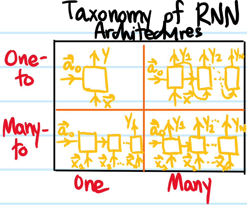
Problem: What does it mean for a collection of feature vectors \(\mathbf x_1,…,\mathbf x_{T}\) to represent a form of sequence data. Give some examples of sequence data.
Solution: It means that the feature vectors are not i.i.d.; indeed, they are in general not a discrete-time Markov chain as each \(\mathbf x_t\) for \(1\leq t\leq T\) can depend on the whole history of \(\mathbf x_{<t}\) that came before it. Examples of sequence data include speech, music, DNA sequences, natural language words, etc.
Problem: Consider the NLP problem of named entity recognition which consists of assigning a binary label \(\hat y\in\{0,1\}\) to every word in an English sentence where \(y=1\) indicates that the word is part of someone’s name. In this case, what is a standard choice for the sequence feature vectors \(\mathbf x_t\)?
Solution: The idea is to employ a one-hot encoding of the words in the sentence with respect to some a priori dictionary of e.g. \(10000\) words in the English language or so. For instance, if “a” is the first word in such a dictionary, then the corresponding one-hot representation of the word “a” would be \(\mathbf x=(1,0,0,…)\in\mathbf R^{10000}\).
Problem: In the broadest sense, what is a recurrent neural network (RNN)? Explain how a simple RNN architecture may be used to analyze the sequence data in the application of named entity recognition described above.
Solution: In the broadest sense, an RNN may be thought of as any function:
that utilizes a so-called hidden state/activation vector \(\mathbf a_t\) (whose dimension is a hyperparameter of the RNN) to remember the history of \(\mathbf x_{<t}\) it has seen so far (typically initialized to \(\mathbf a_{t=1}=\mathbf 0\)). Such a function \(\text{RNN}\) may also depend parametrically on various learnable weights and biases \(\boldsymbol{\theta}\). Different RNN architectures are thus distinguished by the choice of function \(\text{RNN}\).
Intuitively, one can think of an RNN like a sponge that soaks in information, and the corresponding value of its hidden state \(\mathbf a_t\) as a measure of how soaked the sponge currently is. Then, at the next time step, the RNN will increase or decrease its water content based on how wet it currently is \(\mathbf a_{t-1}\) and what external stimulus \(\mathbf x_t\) it receives.
For the named entity recognition task, a simple RNN architecture may be used in which the memory update rule is:
Here, one might take \(\mathbf a_t\in\mathbf R^{512}\) for instance. In that case, the weight matrices and bias vectors \(W_{\mathbf a}\in\mathbf R^{512\times 512},W_{\mathbf x}\in\mathbf R^{512\times 10000},\mathbf b_{\mathbf a}\in\mathbf R^{512}\), and similarly \(W_y\in\mathbf R^{1\times 512},b_y\in\mathbf R\) are all to be learned by the RNN.
Problem: Give a taxonomy of RNN architectures, and classify the above example involving named entity recognition.
Solution: Essentially one has a \(2\times 2\) matrix:
The vanilla RNN architecture described above involving named entity recognition would be classified as a many-to-many RNN architecture.
Problem: Moving on from the example of named entity recognition, consider now a different task of implementing a (word-level) language model using an RNN; how can that be done?
Solution: Using a many-to-many RNN architecture that uses the same hidden state update rule as before:
Moreover, one not only initializes \(\mathbf a_{t=1}=\mathbf 0\), but also \(\mathbf x_{t=1}=\mathbf 0\) and for \(t\geq 2\) takes the previous output as the next input \(\mathbf x_t=\mathbf y_{t-1}\). This same architecture can also be used to generate sequences of text, namely by sampling from the softmax probability distribution \(\mathbf y_t\) at each time step \(t=1,2,…,T\).
Problem: Explain why the simple RNN architecture above suffers from both the vanishing gradient and exploding gradient problems.
Solution: This problem is in fact a general curse of deep neural networks (and RNNs tend to be “deep” because each time step \(t=1,2,…,T\) is analogous to \(1\) layer when the RNN architecture is unrolled). Specifically, when computing gradients of loss functions \(\partial L/\partial\boldsymbol{\theta}\), backpropagation (called backpropagation through time (BPTT) in the context of RNNs) requires chaining \(T\) Jacobian matrices together in a neural net \(T\) layers deep, so if these Jacobians have spectral radii which are systematically \(<1\) or \(>1\), then multiplying them together would lead respectively to a vanishing gradient \(\partial L/\partial\boldsymbol{\theta}\to\mathbf 0\) or exploding gradient \(\partial L/\partial\boldsymbol{\theta}\to\mathbf{\infty}\). All this is to say that the simple RNN architecture will tend to have trouble remembering sequence feature vectors \(\mathbf x_{\ll t}\) that happened a long time ago because again for RNNs, time=layers.
Problem: Explain how the gated recurrent unit(GRU) is a more sophisticated RNN architecture that overcomes the above problems.
Solution: At each time step \(t=1,2,…,T\), a GRU is a map \(\mathbf a_t=\text{GRU}(\mathbf a_{t-1},\mathbf x_t)\) that computes the next hidden state via a sequence of \(4\) computations:
By using the reset gate \(\mathbf r_t\) to remember only relevant information, the GRU is able to retain a much longer-term memory of what has already come before it, thereby mitigating the vanishing gradient problem.
Problem: Show that the long short-term memory (LSTM) architecture is another RNN architecture which, like the GRU, also mitigates the vanishing gradient problem.
Solution: Unlike a GRU which has \(4\) computations and only \(2\) gates, an LSTM is a bit more involved in that it uses \(6\) computations with \(3\) gates (historically, GRUs were invented as a simplification of LSTMs).
Problem: Whatever happened to the output vector \(\hat{\mathbf y}_t\) in the above discussion of the GRU and LSTM recurrent neural network architectures?
Solution: It’s always there, but the exact formula for it depends on the application of interest in a standard way. Usually, one first computes a linear combination \(W_{\mathbf y\mathbf a}\mathbf a_t+\mathbf b_{\mathbf y}\) of the current hidden state, and then applies some activation function to it that depends in the usual way on the application at hand (e.g. sigmoid for binary classification, softmax for multiclass classification).
Problem: Explain how a bidirectional recurrent neural network(BRNN) is an augmentation to the usual RNN architecture.
Solution: Instead of just doing a forward pass in time \(t=1,2,…,T\) through the sequence of feature vectors \(\mathbf x_1,…,\mathbf x_T\), one can also imagine doing a backward pass in time \(t=T,T-1,…,1\) through the same sequence. That is, a BRNN is just \(2\) independent RNNs with hidden states \(\mathbf a_t\) and \(\mathbf a’_t\) respectively, updating according to some specific architectures but in opposite directions through time \(t\):
Of course, the catch with using a BRNN is that one must have access to the entire time series \(\mathbf x_1,…,\mathbf x_T\) up to the total duration \(T\) in order to be able to use it.
Problem: Where and why should one create an __init__.py file?
Solution: Inside a folder/directory that’s meant to be a Python package containing a bunch of Python modules with useful functions, etc. that other Python scripts would be importing from (not strictly necessary as Python \(3.3+\) but still conventional to include).
It executes the first time any module from that package is imported, thus providing a convenient place to run setup code.
Expose functions/classes in internal submodules within the package directly at the package level, simplifying user API.
Defining what gets imported when using wildcard import *.
Problem: (based on this YouTube video) Write some basic Python code to demonstrate how the object-oriented programming(OOP) paradigm works. In particular, show how to create a class, how to initialize attributes of object instances of the class, how to define methods associated to object instances of the class, how child classes can inherit properties of parent classes, and how classes themselves (not just their object instances) can also have class attributes and class methods or static methods.
Solution:
OOP_Fundamentals
In [75]:
classDog:def__init__(self,name,age):# attributes of Dog classself.dog_name=nameself.years_old=agedefadd_one(self,x):# method in classreturnx+1defbark(self):# method in classprint("woof!")defget_name(self):returnself.dog_namedefget_age(self):returnself.years_olddefset_age(self,age):self.years_old=age
False
[<__main__.Student object at 0x7fab84531870>, <__main__.Student object at 0x7fab84532a70>]
Tim
85.0
In [78]:
# Example of inheritance classPet:#parent classdef__init__(self,name,age):self.name=nameself.age=agedefshow(self):print(f"My name is {self.name} and I'm {self.age} years old.")defspeak(self):print("I don't know what to say")classCat(Pet):#child class inherits parent classdef__init__(self,name,age,color):super().__init__(name,age)# reference the super class, aka Pet parent class, view __init__(name, age) as going togetherself.color=colordefspeak(self):print("Meow")defshow(self):print(f"My name is {self.name} and I'm {self.age} years old and my color is {self.color}")classDog(Pet):#child class inherits parent classdefspeak(self):print("Bark")classFish(Pet):passp=Pet("Tim",19)p.show()c=Cat("Bill",38,"Brown")c.show()d=Dog("Jill",25)d.show()f=Fish("Bubbles",29)f.show()print("---")p.speak()c.speak()d.speak()f.speak()
My name is Tim and I'm 19 years old.
My name is Bill and I'm 38 years old and my color is Brown
My name is Jill and I'm 25 years old.
My name is Bubbles and I'm 29 years old.
---
I don't know what to say
Meow
Bark
I don't know what to say
In [ ]:
# Class attributes/methods vs. Instance attributes/methodsclassPerson:number_of_people=0# class attribute (defined w/o using self, thus not specific to an instance of the class)# class attributes would be preferred over just a simple global variable because the class is portable, and so# the value of any class attributes would come along for the ride whenever the class is imported into another filedef__init__(self,name):self.name=namePerson.add_person()@classmethod# decorator defnumber_of_people_(cls):# class method (again, it's for the whole class, not just a specific instance/object of the class)returncls.number_of_people@classmethoddefadd_person(cls):cls.number_of_people+=1p1=Person("Tim")print(Person.number_of_people)p2=Person("Jill")print(p1.number_of_people)print(p2.number_of_people)print(Person.number_of_people)Person.number_of_people=8print(p1.number_of_people)print(p2.number_of_people)print(Person.number_of_people_())
1
2
2
2
8
8
8
In [ ]:
# Static methods classMath:@staticmethod# decorator which is unchanging, no access to an instance hence don't change anythingdefadd5(x):returnx+5@staticmethod# they're basically just regular functions that happen to sit in a class for organizational purposesdefadd10(x):returnx+10@staticmethoddefpr():print("Run!")print(Math.add5(8))print(Math.add10(4))Math.pr()
13
14
Run!
Problem: Explain the purpose of magic methods in OOP Python, and write some code to demonstrate their applications.
Solution: Basically if you want to emulate the behavior of a lot of Python’s built-in classes like being able to concatenate strings using + or getting the length of a list using len(), but with your own classes rather than Python’s built-in classes, then magic methods are the way to go. Another way to put it is that you want to have access to this power of being able to do “operator overload”, so e.g. + is able to mean different things for adding two integers vs. two strings, because in all cases the + is just syntactic sugar for an underlying __add__ magic method that’s defined separately for the int class and the string class.
magic_methods
In [8]:
str1="Hello"str2="World"# The + symbol is syntactic sugar that actually calls the __add__ magic method in the class Stringprint(str1+str2)# To prove that, look at:print(str1.__add__(str2))# Or:int1=1int2=2print(int1+int2)print(int1.__add__(int2))# Similarly for the len function:print(len(str2))print(str2.__len__())
HelloWorld
HelloWorld
3
3
5
5
In [25]:
classCounter:def__init__(self):self.value=42defcount_up(self):self.value+=1defcount_down(self):self.value-=1def__str__(self):returnf"Counter value is currently at {self.value}"def__add__(self,other):#other is always right-side operand (thing coming after the +)ifisinstance(other,Counter):returnself.value+other.valueelse:raiseException("TypeError")count1=Counter()count2=Counter()print(count1)print(count2)# the print function is implicitly going to call the __str__ magic method in the classprint(str(count1))print(str(count2))print("---")print(count1.__str__())print(count2.__str__())count1.count_up()count2.count_down()print(count1)print(count2)print("---")# because implemented __add__ magic methodprint(count1+count2)print(count1.__add__(count2))print(32+count1)
Counter value is currently at 42
Counter value is currently at 42
Counter value is currently at 42
Counter value is currently at 42
---
Counter value is currently at 42
Counter value is currently at 42
Counter value is currently at 43
Counter value is currently at 41
---
84
84
---------------------------------------------------------------------------TypeError Traceback (most recent call last)
Cell In[25], line 38 36print(count1 + count2)
37print(count1.__add__(count2))
---> 38print(32+count1)
TypeError: unsupported operand type(s) for +: 'int' and 'Counter'
In [ ]:
# Anytime one is writing a Python class, it's almost always a good idea to include __str__ and __repr__ magic methods # in the classclassCar:def__init__(self,make,model,year):self.make=makeself.model=modelself.year=yeardef__str__(self):returnf"{self.year}{self.make}{self.model}"def__repr__(self):# stands for "representation"returnf"Car(make='{self.make}', model='{self.model}', year={self.year})"# this is the standard way to write a __repr__ method, namely "Class(attributes)"my_car=Car("Toyota","Corolla",2021)print(str(my_car))print(repr(my_car))
2021 Toyota Corolla
Car(make='Toyota', model='Corolla', year=2021)
In [ ]:
classInventoryItem:""" A class to demonstrate operator overloading """def__init__(self,name,quantity):self.name=nameself.quantity=quantitydef__repr__(self):returnf"InventoryItem(name='{self.name}', quantity='{self.quantity}')"# Arithmetic operatorsdef__add__(self,other):ifisinstance(other,InventoryItem)andself.name==other.name:returnInventoryItem(self.name,self.quantity+other.quantity)# or other.nameraiseValueError("Cannot add iterms with different names")def__sub__(self,other):ifisinstance(other,InventoryItem)andself.name==other.name:ifself.quantity>=other.quantity:returnInventoryItem(self.name,self.quantity-other.quantity)raiseValueError("Cannot subtract more than the available quantity.")raiseValueError("Cannot subtract items of different types.")def__mul__(self,factor):ifisinstance(factor,(int,float)):returnInventoryItem(self.name,int(self.quantity*factor))raiseValueError("Factor must be an int or a float")def__truediv__(self,factor):ifisinstance(factor,(int,float))andfactor!=0:returnInventoryItem(self.name,self.quantity/factor)raiseValueError("Factor must be non-zero int or float")# Comparison operators:def__eq__(self,other):ifisinstance(other,InventoryItem):returnself.name==other.nameandself.quantity==other.quantityraiseValueError("Cannot compare items of different types.")def__lt__(self,other):ifisinstance(other,InventoryItem)andself.name==other.name:returnself.quantity<other.quantityreturnValueError("Cannot compare items of different types.")def__gt__(self,other):ifisinstance(other,InventoryItem)andself.name==other.name:returnself.quantity>other.quantityraiseValueError("Cannot compare items of different types.")def__ne__(self,other):returnnot(self==other)# uses the __eq__ magic methoditem1=InventoryItem("Apples",80)item2=InventoryItem("Oranges",20)item3=InventoryItem("Apples",33)print(item1+item3)print(item1-item3)print(item2*3)print(item1<item3)print(item1!=item2)
# more examples of magic methods with a singly linked list exampleclassNode:def__init__(self,value):self.value=valueself.next=NoneclassLinkedList:def__init__(self):self.head=Noneself.size=0def__len__(self):returnself.sizedef__getitem__(self,index):ifindex<0orindex>=self.size:raiseIndexError("Index out of range.")current=self.headfor_inrange(index):current=current.nextreturncurrent.valuedef__setitem__(self,index,value):ifindex<0orindex>=self.size:raiseIndexError("Index out of range.")current=self.headfor_inrange(index):current=current.nextcurrent.value=valuedef__delitem__(self,index):ifindex<0orindex>=self.size:raiseIndexError("Index out of range.")ifindex==0:self.head=self.head.nextelse:current=self.headfor_inrange(index-1):current=current.nextcurrent.next=current.next.nextself.size-=1def__contains__(self,value):current=self.headwhilecurrent:ifcurrent.value==value:returnTruecurrent=current.nextreturnFalsedefappend(self,value):# not a magic methodnew_node=Node(value)ifnotself.head:self.head=new_nodeelse:current=self.headwhilecurrent.next:current=current.nextcurrent.next=new_nodeself.size+=1def__str__(self):values=[]current=self.headwhilecurrent:values.append(str(current.value))current=current.nextreturn" -> ".join(values)LL=LinkedList()LL.append(10)LL.append(20)LL.append(30)print(LL)print(len(LL))print(LL[2])LL[0]=22print(LL)delLL[1]print(LL)print(30inLL)
10 -> 20 -> 30
3
30
22 -> 20 -> 30
22 -> 30
True
In [ ]:
classDatabaseConnection:def__init__(self,db_name):self.db_name=db_nameself.connected=Falsedef__enter__(self):self.connected=Trueprint(f"Connected to the database '{self.db_name}'.")returnselfdef__exit__(self,exc_type,exc_value,traceback):self.connected=Falseprint(f"Disconnected from the database '{self.db_name}'.")ifexc_type:print(f"An exception occurred: {exc_value}")returnTruewithDatabaseConnection("ExampledDB")asdb:# context managerprint(f"Is connected? {db.connected}")
Connected to the database 'ExampledDB'.
Is connected? True
Disconnected from the database 'ExampledDB'.
For more magic methods, you can starting type the double underscore, and see what VS Code IDE suggests:
Problem: Write Python code to demonstrate some applications of decorators, generators and context managers.
Solution: A decorator (@) is basically a wrapper function \(w\) that itself takes in some function \(f\) and maps it to a “wrapped” version \(w(f)\) of \(f\) with greater functionality but without cluttering the logic of \(f\) itself. A generator (yield) is also a function which is a bit like a discrete-time Markov chain. A context manager (with) guarantees that a program will exit even if there were errors during its execution.
Decorators_Generators_Context_Managers
In [1]:
# Decoratorsdeffunc(f):defwrapper():print("Started")f()print("Ended")returnwrapperdeffunc2():print("I am func2")deffunc3():print("I am func3")x=func(func3)y=func(func2)print(x)x()y()
<function func.<locals>.wrapper at 0x7fa7335cb2e0>
Started
I am func3
Ended
Started
I am func2
Ended
In [2]:
func3=func(func3)# not ideal to write this line of code :(func2=func(func2)func3()func2()
Started
I am func3
Ended
Started
I am func2
Ended
In [3]:
# Decorators are a solution@funcdeffunc3():print("I am func3")func3()func2()# anytime want to create a Python decorator function, need to return the "wrapper"
Started
I am func3
Ended
Started
I am func2
Ended
In [4]:
# But suppose func2 had an argument x@funcdeffunc2(x):print(x)func2(3)
---------------------------------------------------------------------------TypeError Traceback (most recent call last)
Cell In[4], line 6 2@func 3deffunc2(x):
4print(x)
----> 6func2(3)TypeError: func.<locals>.wrapper() takes 0 positional arguments but 1 was given
In [5]:
# One could just redefine wrapper() to be wrapper(x):deffunc(f):defwrapper(x):print("Started")f(x)print("Ended")returnwrapper@funcdeffunc2(x):print(x)func2(4)
Started
4
Ended
In [6]:
# But then this throws an error for func3 which currently takes no arguments:@funcdeffunc3():print("I am func3")func3()
# Solution is to use an unpack operator *:deffunc(f):defwrapper(*args,**kwargs):# within the function scope, args is a tuple and kwargs is a dictionaryprint("Started")rv=f(*args,**kwargs)print("Ended")returnrvreturnwrapper@funcdeffunc2(x,y):print(x)returny@funcdeffunc3():print("hey")x=func2(5,6)print(x)
# Generatorsx=[n**2forninrange(10000)]forelinx:print(el)# notice how in this application just want to print one value at a time# the list is so large, all of RAM is being used!
# However, Python has a simpler way to implement a generator function, namely via the yield keyworddefgen(n):foriinrange(n):yieldi**2#yield = pauseg=gen(1000)print(type(g))foriing:print(i)
<class 'generator'>
0
1
4
9
...
996004
998001
In [12]:
# Alternatively, can use the next method:g=gen(1000)print(next(g))print(next(g))print(next(g))print(next(g))
0
1
4
9
In [13]:
# we can explicitly unravel the generator scope (previously a for loop) as a sequence of yield statementsdefgen():yield1yield3yield5g=gen()print(next(g))print(next(g))print(next(g))print(next(g))
# Comparison between lists and generator memory usage:importsysdefgen(n):foriinrange(n):yieldi**2x=[i**2foriinrange(10000)]g=gen(10000)print(sys.getsizeof(x))print(sys.getsizeof(g))
# this code here is equivalent to the above code:withopen("file.txt","a")asfile:file.write("hello")
In [17]:
classFile:def__init__(self,filename,method):self.file=open(filename,method)def__enter__(self):print("Enter")returnself.filedef__exit__(self,type,value,traceback):print(f"{type}, {value}, {traceback}")print("Exit")self.file.close()iftype==Exception:returnTrue# tell Python exception was gracefully handled, program doesn't need to crash anymorewithFile("file.txt","w")asf:print("Middle")f.write("hello!")raiseFileExistsError()
Enter
Middle
<class 'FileExistsError'>, , <traceback object at 0x7fa7328df800>
Exit