In this interview, well-known theoretical physicist Frank Wilczek commented that “still to this day I think the quantum theory of angular momentum is one of the absolute pinnacles of human achievement. Just beautiful”. The purpose of this post is to give a flavor of why Wilczek might have thought that.
As (orbital/spin/total) angular momentum should be an observable, it therefore should arise from a smooth projective unitary representation \(\phi^{\infty}\) of some group acting on suitable state spaces \(\mathcal H\cong L^2(\textbf R^3\to\textbf C,d^3\textbf x)\). Unsurprisingly, that group is \(SO(3)\) with \(\phi^{\infty}:SO(3)\to PU(\mathcal H)\) being defined by \(\langle\textbf x|\phi^{\infty}_R|\psi\rangle:=\langle R^{-1}\textbf x|\psi\rangle\) where also \(R^{-1}=R^T\) (although it’s quite intuitive why it must be \(R^{-1}\) rather than \(R\), one can also check that only \(R^{-1}\) allows the homomorphism property \(\phi^\infty_{R_2R_1}=\phi^\infty_{R_2}\circ\phi^{\infty}_{R_1}\) to be satisfied). The induced Lie algebra representation is then \(\dot{\phi}^{\infty}_1:\frak{so}\)\((3)\to\frak u\)\((\mathcal H)/i\textbf R1\) given by \(\dot{\phi}^{\infty}_1(\tilde J)=\left(\frac{\partial}{\partial\theta}\right)_{\theta=0}\phi^{\infty}_{e^{\tilde{J}\theta}}\), so that one has the angular directional derivative:
\[\langle\textbf x|\dot{\phi}^{\infty}_1(\tilde J)|\psi\rangle=-\tilde{J}\textbf x\cdot\frac{\partial\langle\textbf x|\psi\rangle}{\partial\textbf x}\]
Letting \(\tilde{J}_1,\tilde J_2,\tilde J_3\in\frak{so}\)\((3)\) be the standard generators of \(\frak{so}\)\((3)\) (i.e. \((\tilde J_i)_{jk}=\varepsilon_{ijk}\)). Consider substituting \(\tilde J:=\tilde J_3\) for instance. Then clearly, one has:
\[\langle\textbf x|\dot{\phi}^{\infty}_1(\tilde J_3)|\psi\rangle=-\frac{\partial\langle\textbf x|\psi\rangle}{\partial\phi}\]
with \(\phi\) the usual cylindrical coordinate about the \(z\)-axis. It is instructive to prove this by writing \(\textbf x=\rho\hat{\boldsymbol{\rho}}_{\phi}+z\hat{\textbf k}\), \(\tilde J_3\textbf x=\hat{\textbf k}\times\textbf x\) and using the standard expression of the gradient in cylindrical coordinates \(\frac{\partial\langle\textbf x|\psi\rangle}{\partial\textbf x}=\frac{\partial\langle\textbf x|\psi\rangle}{\partial\rho}\hat{\boldsymbol{\rho}}_\phi+\frac{1}{\rho}\frac{\partial\langle\textbf x|\psi\rangle}{\partial\phi}\hat{\boldsymbol{\phi}}_{\phi}+\frac{\partial\langle\textbf x|\psi\rangle}{\partial z}\hat{\textbf k}\). Finally, to recover the angular momentum observables, one just does the usual multiply by \(i\hbar\), so for instance one has the familiar \(\langle\textbf x|L_3|\psi\rangle=-i\hbar\frac{\partial\langle\textbf x|\psi\rangle}{\partial\phi}\). This should be compared with formulas such as \(\langle\textbf x|\textbf P|\psi\rangle=-i\hbar\frac{\partial\langle\textbf x|\psi\rangle}{\partial\textbf x}\) and \(H|\psi\rangle=i\hbar\frac{\partial|\psi\rangle}{\partial t}\).
The commutation relations \([\tilde J_i,\tilde J_j]=\varepsilon_{ijk}\tilde J_k\) for \(\frak{so}\)\((3)\) are just an application of the Jacobi identity for \(\textbf R^3\) with the cross product \(\times\). It suffices to show \([\tilde J_1,\tilde J_2]=\tilde J_3\) for example. We have: \([\tilde J_1,\tilde J_2]\textbf x=\tilde J_1\tilde J_2\textbf x-\tilde J_2\tilde J_1\textbf x=\hat{\textbf i}\times(\hat{\textbf j}\times\textbf x)-\hat{\textbf j}\times(\hat{\textbf i}\times\textbf x)=(\hat{\textbf i}\times\hat{\textbf j})\times\textbf x=\hat{\textbf k}\times\textbf x=\tilde J_3\times\textbf x\). The commutator algebra for the angular momentum observables are then directly inherited from the commutation relations for \(\frak{so}\)\((3)\) thanks to the fact that \(\dot{\phi}^\infty_1\) is a Lie algebra representation. To wit, consider \([J_i,J_j]=[i\hbar\dot{\phi}^\infty_1(\tilde J_1),i\hbar\dot{\phi}^\infty_1(\tilde J_2)]=(i\hbar)^2[\dot{\phi}^\infty_1(\tilde J_1),\dot{\phi}^\infty_1(\tilde J_2)]=(i\hbar)^2\dot{\phi}^\infty_1([\tilde J_1,\tilde J_2])=(i\hbar)^2\dot{\phi}^\infty_1(\varepsilon_{ijk}\tilde J_k)=i\hbar\varepsilon_{ijk}J_k\). Or, on a more abstract level, it is clear that we have the isomorphism of Lie algebras \((\textbf R^3,\times)\cong(\frak{so}\)\((3),[,])\).
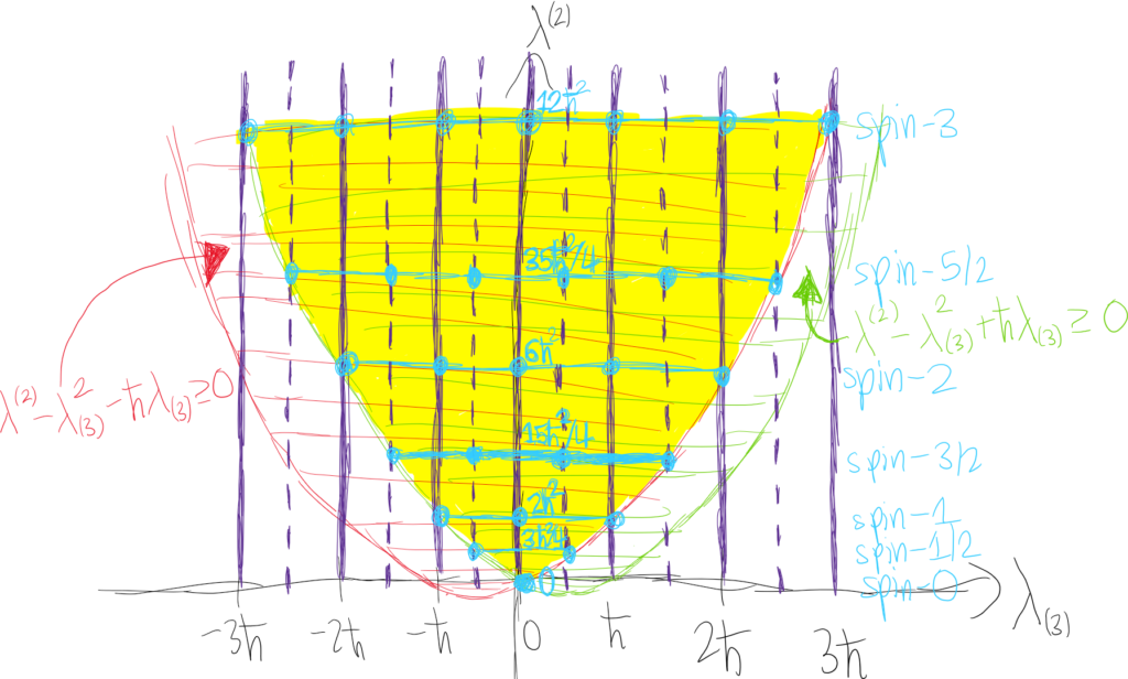
Anyways, armed with the commutator algebra \([J_i,J_j]=i\hbar\varepsilon_{ijk}J_k\), the spectrum \(\Lambda_{J_3}\) can be deduced. Letting \(\textbf J^2:=J_1^2+J_2^2+J_3^2\) be the Casimir invariant so that \([\textbf J^2,J_i]=0\), this means one can only know (i.e. measure with \(100\%\) certainty) the total angular momentum and angular momentum along one specific direction \(\hat{\textbf n}\). Arbitrarily orienting the coordinate axes so that \(\hat{\textbf n}:=\hat{\textbf k}\), this means the angular momentum \(J_3\) of the quantum particle along the \(z\)-axis is known and therefore is unknown in the \(xy\)-plane. Now, notice that \(\textbf J^2-J_3^2=J_1^2+J_2^2\). The right-hand side is a sum of squares, so there are two factorizations possible: \(J_1^2+J_2^2=(J_1+iJ_2)(J_1-iJ_2)+i[J_1,J_2]=(J_1-iJ_2)(J_1+iJ_2)+i[J_2,J_1]\). However, we’ve already worked out that \([J_1,J_2]=-[J_2,J_1]=i\hbar J_3\). Defining the mutually adjoint raising and lowering ladder operators \(J_{\pm}:=J_1\pm iJ_2\), this means that \(\textbf J^2-J_3^2+\hbar J_3=J_+J_-\) and \(\textbf J^2-J_3^2-\hbar J_3=J_-J_+\). In both cases, notice that both \(J_+J_-\) and \(J_-J_+\) are Hermitian and positive semi-definite (being of the standard SVD form, analogous to the number operator for the quantum harmonic oscillator). Thus, if \(|\lambda^{(2)},\lambda_{(3)}\rangle\) is a simultaneous eigenstate of \(\textbf J^2\) and \(J_3\) with the obvious eigenvalues, then the singular values must satisfy \(\lambda^{(2)}-\lambda_{(3)}^2+\hbar\lambda_{(3)}\geq 0\) and \(\lambda^{(2)}-\lambda_{(3)}^2-\hbar\lambda_{(3)}\geq 0\) (this has a nice geometric interpretation with two parabolas and the intersection in the middle region). The result is that for a given total angular momentum (squared) \(\lambda^{(2)}\), the angular momentum \(\lambda_{(3)}\) in the \(z\)-direction can only lie in an interval of width \(\sqrt{\hbar^2+4\lambda^{(2)}}-\hbar\) centered around \(\lambda_{(3)}=0\).
Now the part that I’m still figuring out how to understand deeply/motivate. Just as when one factorizes the Hamiltonian \(H_{\text{QHM}}\) of the quantum harmonic oscillator and realized that the factors turn out to act as raising and lowering operators for \(H_{\text{QHM}}\), so here the same phenomenon occurs. I feel that it depends not just on the fact that one is dealing with a sum of squares, but also works in both cases because the commutator is really simple. Once you know that, the proof is straightforward:
\[J_3J_+|\lambda^{(2)},\lambda_{(3)}\rangle=J_3J_1|\lambda^{(2)},\lambda_{(3)}\rangle+iJ_3J_2+|\lambda^{(2)},\lambda_{(3)}\rangle\]
The intuition here is that it would be really nice if the \(J_3\) could act on the state instead since we know exactly what it will do \(J_3|\lambda^{(2)},\lambda_{(3)}\rangle=\lambda_{(3)}|\lambda^{(2)},\lambda_{(3)}\rangle\). So to be able to make this happen, the commutator emerges naturally as a necessity to compute, which fortunately we already know. This yields:
\[J_3J_+|\lambda^{(2)},\lambda_{(3)}\rangle=(\lambda_{(3)}+\hbar)J_+|\lambda^{(2)},\lambda_{(3)}\rangle\]
And by a similar computation, \(J_3J_-|\lambda^{(2)},\lambda_{(3)}\rangle=(\lambda_{(3)}-\hbar)J_-|\lambda^{(2)},\lambda_{(3)}\rangle\). Finally, since \([\textbf J^2,J_{\pm}]=0\) (as each of the \(J_i\) commute with \(\textbf J^2\)), this means that \(\textbf J^2J_{\pm}|\lambda^{(2)},\lambda_{(3)}\rangle=J_{\pm}\textbf J^2|\lambda^{(2)},\lambda_{(3)}\rangle=\lambda^{(2)}J_{\pm}|\lambda^{(2)},\lambda_{(3)}\rangle\). The key result is therefore that \(J_+\) and \(J_-\) can both be thought of as increasing or decreasing the total angular momentum of the system along the \(z\)-axis but without changing the total angular momentum \(\textbf J^2\). The mere existence of the ladder operators means ultimately that the end result is as depicted in the picture below. Read the vertical axis as imposing the total amount of angular momentum (squared) and the horizontal axis as imposing the amount of angular momentum in the \(z\)-direction, with the valid angular momentum eigenstates forming a hexagonal lattice of sorts.
In physical space \(\textbf R^3\), the quantized angular momenta vectors allowed can be represented by this cross-section of the \(\rho\) vs. \(z\) plane. Below is for \(j=0,1/2,1,…,5\):
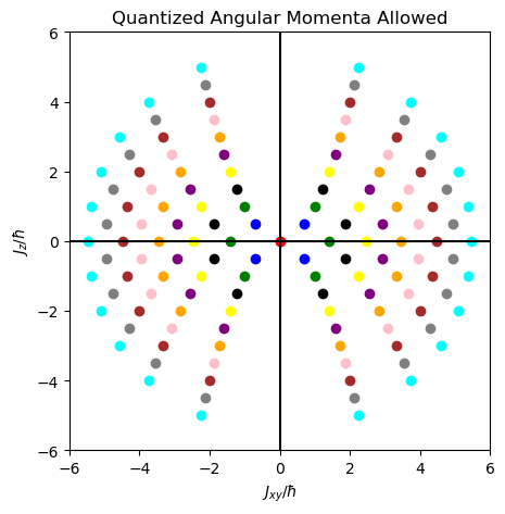
Focusing on the highest-weight states \(m_j=j\) (the inner parabolas in the diagram), for \(j=1/2\) the dark blue dots are inclined at the magic angle \(\theta_{1/2}=54.7^{\circ}\) from the \(z\)-axis, while for the \(j=1\) highest-weight states the angle is \(\theta_1=45^{\circ}\) as is intuitively clear from the plot. In general, it is straightforward to show that for that highest-weight state \(|j(j+1)\hbar ^2,j\hbar\rangle\), the angle decreases as \(\cos(\theta_j)=\sqrt{\frac{j}{j+1}}\) so that \(\lim_{j\to\infty}\theta_j=0\) (aside, one immediate conjecture is that there exists some relation between these angles \(\theta_j\) and the position representations \(\langle\textbf x|j(j+1)\hbar^2,j\hbar\rangle\) of these angular momentum eigenstates since the magic angle satisfies \(P_2(\cos(\theta_{1/2}))=0\) and if I remember correctly the angular momentum eigenstates are written in terms of spherical harmonics in the position representation which are defined via Legendre functions \(P_j^{m_j}(\cos(\theta))\) of the first kind…does it correspond to some kind of conical angular node?
If one wished, it is straightforward to compute the following explicit normalization constants (using the Condon-Shortley phase convention):
\[J_+|j(j+1)\hbar^2,m_j\hbar\rangle=\sqrt{j(j+1)-m_j(m_j+1)}\hbar|j(j+1)\hbar^2,(m_j+1)\hbar\rangle\]
\[J_-|j(j+1)\hbar^2,m_j\hbar\rangle=\sqrt{j(j+1)-m_j(m_j-1)}\hbar|j(j+1)\hbar^2,(m_j-1)\hbar\rangle\]
which will be real because \(-j\leq m_j\leq j\) as \(j\in\textbf N/2\) is by definition the highest weight (or spin) of the irreducible representation for which \(J_+|\lambda^{(2)},j\rangle=0\).
The Hamiltonian \(H_{RR}\) of a rigid rotor (rigid means no vibration, so one can safely set the potential energy \(V=0\)) consists entirely of rotational kinetic energy about its center of mass:
\[H_{RR}=\frac{1}{2}\left(\frac{J_1^2}{I_1}+\frac{J_2^2}{I_2}+\frac{J_3^2}{I_3}\right)\]
where \(I_1,I_2,I_3\) are its principal moments of inertia. Assuming \(z\)-axisymmetry \(I_1=I_2=I\), one has:
\[H_{\text{rigid rotor}}=\frac{1}{2}\left(\frac{J^2}{I}+\left(\frac{1}{I_3}-\frac{1}{I}\right)\textbf J_3^2\right)\]
At this point, the spectrum \(\Lambda_{H_{\text{rigid rotor}}}\) of kinetic energies is easy to read off, where as usual \(j\in\textbf N/2\) and \(m_j\in\{-j,…,j\}\):
\[E_{j,m_j}=\frac{\hbar^2}{2I}\left(j(j+1)+\left(\frac{I}{I_3}-1\right)m_j^2\right)\]
The ground state energy of the rigid rotor fixed in free space is thus \(E_{0,0}=0\) corresponding to no kinetic energy. In general, because \(I_3\ll I\), it follows that the lowest energy states should have \(m_j=0\) (i.e. no angular momentum about the \(z\)-axis so one can visualize how the rigid rotor necessarily ought to be spinning). This can only occur for integer total angular momenta \(j\in\textbf N\subseteq\textbf N/2\) where now:
\[E_{j,0}=j(j+1)\frac{\hbar^2}{2I}\]
Thus, the constraint \(j\in\textbf N\) means that if the rigid rotor is in state \(|j(j+1)\hbar^2,0\rangle\), then the smallest energetic transition it can make is by \(\Delta j=1\) and not \(\Delta j=1/2\) (EDIT: I’m so dumb bruh why was I even thinking this…clearly there ain’t such a thing as a “half-raising” or “half-lowering” operator). The smallest energy of the corresponding photon it can absorb/emit is (basically, recall that anytime one has a quadratic map \(j\mapsto j^2\) then the first differences \(\Delta j\propto j\)):
\[\Delta E^j_{j-1}=E_{j,0}-E_{j-1,0}=\frac{j\hbar^2}{I}\]
with angular frequency \(\omega^j_{j-1}=\Delta E^j_{j-1}/\hbar=j\hbar/I=j\omega^1_0\). If one models a carbon monoxide \(\text{CO}\) molecule as a rigid rotor in one of these low energy states, then about the center of mass one has \(I=\mu R^2\) where \(\mu=\frac{12\times 16}{12+16}\text{ u}\) is the reduced mass and \(R=112.8\text{ pm}\) is the bond length. These combine to yield a base photon frequency of \(f^1_0=\omega^1_0/2\pi=115.8\text{ GHz}\), which is close to the experimental \(f^1_0=113.17\text{ GHz}\), a very important spectral frequency in astronomy for the study of interstellar gas. One might inquire by what factor the angular velocity \(\Omega_j\) of the molecule’s rotation is related to the angular frequency \(\omega^j_{j-1}\) of photons absorbed/emitted. Since it was already mentioned that the rigid rotor in these low energy states does not rotate at all in the \(z\)-direction \(m_j=0\), it follows that \(|\textbf J|=I\Omega_j\), but we also know that \(|\textbf J|=\sqrt{j(j+1)}\hbar=j\hbar + O_{j\to\infty}(1)\) so \(\Omega_j\approx \omega^j_{j-1}\) as \(j\to\infty\) which is to be expected (e.g. from Maxwell’s equations applied to a rotating electric dipole), although if \(j\) gets too large then there may eventually be some \(m_j=\pm 1/2\) states popping up too?