Classically, if one takes a trajectory \(\textbf x(t)\) and reflects it about the origin to obtain the reflected trajectory \(\textbf x'(t)=-\textbf x(t)\), then the momentum of the particle \(\textbf p=m\dot{\textbf x}\) is correspondingly reflected \(\textbf p’=m\dot{\textbf x’}=-m\dot{\textbf x}=-\textbf p\). Thus, a parity transformation \(\textbf x\mapsto -\textbf x\) maps the entire state \((\textbf x,\textbf p)\) of the particle in phase space to \((-\textbf x,-\textbf p)\).
When working with quantum mechanics on \(\textbf R^3\) so that \(\mathcal H\cong L^2(\textbf R^3\to\textbf C,d^3\textbf x)\), one defines the discrete parity operator \(\Pi\in U(\mathcal H)\cap i\frak u\)\((\mathcal H)\) to be a unitary, Hermitian, and involutory operator \(\Pi=\Pi^{\dagger}=\Pi^{-1}\) that acts on states \(|\psi\rangle\in\mathcal H\) via a spatial inversion of their wavefunction:
For instance, for an \(\textbf X\)-eigenstate \(|\psi\rangle=|\textbf x\rangle\), the above definition implies that \(\Pi|\textbf x\rangle=|-\textbf x\rangle\) whereas for a \(\textbf P\)-eigenstate \(|\psi\rangle =|\textbf p\rangle\) one has \(\Pi|\textbf p\rangle =|-\textbf p\rangle\) thanks to \(\langle -\textbf x|\textbf p\rangle=e^{i(-\textbf x)\cdot\textbf p/\hbar}/(2\pi\hbar)^{3/2}=e^{i\textbf x\cdot(-\textbf p)/\hbar}/(2\pi\hbar)^{3/2}=\langle\textbf x|-\textbf p\rangle\) so it completely mirrors the classical parity transformation.
Noting for arbitrary \(|\psi\rangle\in\mathcal H\) that \(\langle\psi|\Pi^{\dagger}\textbf X\Pi|\psi\rangle=-\langle\psi|\textbf X|\psi\rangle\), this yields \(\Pi^{\dagger}\textbf X\Pi=-\textbf X\). One can compute that the momentum operator \(\textbf P\) conjugates via the parity operator \(\Pi\) in exactly the same manner as the position operator \(\textbf X\), namely \(\Pi^{\dagger}\textbf P\Pi=-\textbf P\), so \(\textbf P\) is said to be a vector operator (the position operator \(\textbf X\) is also trivially a vector operator as the whole definition of vector operator is based on how \(\textbf X\) itself conjugates via \(\Pi\)). It follows that the orbital angular momentum \(\textbf L:=\textbf X\times\textbf P\) does not conjugate via \(\Pi\) in the same manner, but instead \(\Pi^{\dagger}\textbf L\Pi=\Pi^{\dagger}\textbf X\times\textbf P\Pi=(-\textbf X)\times(-\textbf P)=\textbf X\times\textbf P=\textbf L\) which can be taken to define a pseudovector operator (this is nothing new; in classical mechanics, if one views the dynamics of a system in a “mirror” (not the kind hanging on one’s wall, but really a sort of “inverting mirror”), the angular momentum vector \(\textbf L=\textbf x\times\textbf p\) is also a pseudovector precisely because both \(\textbf x\) and \(\textbf p\) are vectors and two wrongs make a right). The spin angular momentum \(\textbf S\) and the total angular momentum \(\textbf J\) are also pseudovector operators. There is of course also the notion of a scalar operator (e.g. the non-relativistic kinetic energy operator \(T:=\textbf P^2/2m\)) and a pseudoscalar operator (e.g. the dot product of a vector and a pseudovector operator \(\textbf P\cdot\textbf L\)) (and more generally tensor operators (especially spherical tensor operators as in the Wigner-Eckart theorem) and pseudotensor operators). The following table summarizes these ideas pretty well:
where always keep in mind that the reference is based on the position operator \(\textbf X\) transforming under spatial rotations as \(e^{i\Delta\boldsymbol{\phi}\cdot\textbf L/\hbar}\textbf Xe^{-i\Delta\boldsymbol{\phi}\cdot\textbf L/\hbar}\mapsto e^{\Delta\boldsymbol{\phi}\cdot\boldsymbol{\mathcal{L}}}\textbf X\) and under parity as \(\Pi^{\dagger}\textbf X\Pi=-\textbf X\).
Given that \(\Pi\in U(\mathcal H)\cap i\frak u\)\((\mathcal H)\), it follows that \(\Lambda_{\Pi}\subseteq U(1)\cap \textbf R=\{-1,1\}\) and indeed \(\Pi\)-eigenstates with definite parity \(+1\) are called even while those with \(-1\) are called odd.
We know that a Hamiltonian \(H\) is rotationally symmetric iff it fulfills the first criteria in the table above for being a scalar operator (and consequently conserves angular momentum). One can also consider situations in which the Hamiltonian \(H\) fulfills the second criteria (independent of whether or not it also fulfills the first), namely whether or not \([H,\Pi]=0\) (in which case parity is conserved in all processes governed by that Hamiltonian \(H\)). For instance, it is known that \([H_{\text{electromagnetism}},\Pi]=[H_{\text{strong interaction}},\Pi]=[H_{\text{gravity}},\Pi]=[H_{\text{Higgs}},\Pi]=0\) but a famous experiment of Wu et al. showed that \([H_{\text{weak interaction}},\Pi]\neq 0\) so parity is conserved in all electromagnetic or strong interactions (giving rise to spectroscopic selection rules, etc.) but not in weak interactions (e.g. parity conservation is violated in radioactive \(\beta\) decays).
For instance, the Hamiltonian of both the quantum harmonic oscillator and any central potential are automatically parity-conservative, so energy eigenspaces have definite parity; in the case of the former one can use ladder operators to show that the energy eigenstates \(|0\rangle,|1\rangle,…\) (as labelled by the eigenvalue of the number operator) have alternating parity \(\Pi|n\rangle=(-1)^n|n\rangle\) whereas in any central potential one has \(\Pi|n,\ell,m_{\ell}\rangle =(-1)^{\ell}|n,\ell,m_{\ell}\rangle\) as one can show by just looking at how the highest weight spherical harmonics \(Y_{\ell}^{\ell}(\theta,\phi)=e^{i\ell\phi}\sin^{\ell}\theta\) transform under \((\theta,\phi)\mapsto (\pi-\theta,\phi+\pi)\) and using the ladder operators \(L_{\pm}\) to prove the \(m_{\ell}\)-independence of the parity.
As an application of the above idea, if one has a system of two quantum particles interacting via a potential energy \(V=V(|\textbf X_1-\textbf X_2|)\), then by boosting into the center-of-mass frame it becomes clear that such a Hamiltonian will be rotationally symmetric with respect to their relative position \(\textbf X:=\textbf X_1-\textbf X_2\) and so the \(H\)-eigenstates of such a system will look like a radial part times a spherical harmonic. The parity operator on \(\mathcal H=\mathcal H_1\otimes\mathcal H_2\) is \(\Pi:=\Pi_1\otimes\Pi_2\), so if the composite state is in a \(\Pi\)-eigenstate \(|\pi\rangle=|\pi_1\rangle\otimes|\pi_2\rangle\), then \(\Pi|\pi\rangle=\Pi_1\otimes\Pi_2|\pi_1\rangle\otimes|\pi_2\rangle\) so in particular \(\pi=\pi_1\pi_2(-1)^{\ell}\) (not sure how fully airtight that argument is but the result is correct for the intrinsic parities which derive from quantum field theory).
Example: if a \(\pi^-\) pion scatters inelastically off a deuteron \(d^+=(p^+,n^0)\) to create two neutrons \(n^0\) so that \(\pi^-+d^+\to n^0+n^0\), then because the weak interaction is not involved, one must have conservation of parity \(\pi’=\pi\). But \(\pi=\pi_{\pi^-}\pi_{d^+}(-1)^{\ell_{(\pi^-,d^+)}}\) and \(\pi’=\pi^2_{n^0}(-1)^{\ell_{(n^0,n^0)}}\). Now if one accepts that \(\ell_{(\pi^-,d^+)}=0\), that \(\pi_{d^+}=\pi_{p^+}\pi_{n^0}(-1)^{\ell_{(p^+,n^0)}}\), that \(\pi_{p^+}=\pi_{n^0}\) due to an approximate, internal \(SU(2)\) isospin symmetry of the Standard Model, that \(\ell_{(p^+,n^0)}=0\) is in an “\(s\)-wave bound state”, and that \(\ell_{(n^0,n^0)}=1\) in order to conserve total angular momentum and respect the fermionic nature of the identical neutrons \(n^0\) created, then one deduces \(\pi_{\pi^-}=-1\) is a pseudoscalar particle (since it is given that \(s_{\pi^-}=0\)). Thus, this example demonstrates that parity conservation (together with angular momentum conservation in this case) can be a useful tool for deducing the intrinsic parities of hadrons in experiments.
Time Reversal
Again, begin with a discussion of classical mechanics first before moving onto the quantum mechanical case. Here, if one takes a trajectory \(\textbf x(t)\) and, rather than negating the output as was done for a parity transformation, negate the input instead to obtain the time-reversed trajectory \(\textbf x'(t)=\textbf x(-t)\). This correspondingly means that \(\textbf p'(t)=m\dot{\textbf x}'(t)=-\textbf p(-t)\) and \(\textbf L'(t)=-\textbf L(-t)\), etc. Note that electromagnetic fields also transform under time reversal \(\rho\mapsto\rho,\textbf J\mapsto -\textbf J,\textbf E\mapsto\textbf E,\textbf B\mapsto -\textbf B\).
Since the phrase “time reversal” and the Greek letter “theta” \(\Theta\) both start with the letter “t”, it seems customary to denote the quantum mechanical time reversal operator by \(\Theta\). One thing that’s immediately strange is that because the Schrodinger equation is first-order in time, it is basically like a heat/diffusion equation whose solution space is certainly not closed under “naive” time reversal \(|\psi(t)\rangle\mapsto |\psi(-t)\rangle\). Instead, thanks to the factor of \(i\) it turns out that the correct definition of the time reversal operator \(\Theta\) is:
\[\Theta|\psi(t)\rangle:=|\psi(-t)\rangle^*\]
Where one can now check that \(i\hbar\frac{\partial}{\partial t}\Theta\psi=H\Theta\psi\) is indeed a valid solution of the Schrodinger equation. One can check that this definition ensures that it behaves in accordance with classical time reversal, for instance:
\[\]
For all the training we’ve done with linear algebra, here it will be necessary to work with antilinear algebra (the two coincide over real vector spaces, but unfortunately Hilbert spaces are complex in QM).
In number theory, the fundamental theorem of arithmetic clarifies why prime numbers are so important, namely that they form a “multiplicative basis” with which one can uniquely factorize any positive integer \(n\in \textbf Z^+\). In the same spirit, Schur’s lemma provides for representation theory roughly the analog of what the fundamental theorem of arithmetic provides for number theory, namely instead of prime numbers being in the spotlight it is the irreducible representations of a group \(G\) which are now in the spotlight. For this reason, I like to informally think of Schur’s lemma as the “fundamental theorem of representation theory” since there is a whole edifice of results (e.g. the Schur orthogonality relations for characters, the Peter-Weyl theorem for compact Lie groups, the decomposition of representation tensor products into direct sums of irreducible subrepresentations, etc.) built from Schur’s lemma.
Recall that given a group \(G\), two \(G\)-representations \(\phi_1:G\to GL(V_1)\), \(\phi_2:G\to GL(V_2)\) on vector spaces \(V_1,V_2\) are considered isomorphic \(G\)-representations iff there exists a vector space isomorphism \(L:V_1\to V_2\) that conjugates between the two \(G\)-representations for all symmetries \(g\in G\), i.e. \(\phi_2(g)=L\phi_1(g)L^{-1}\). Equivalently, one can view \(L\) as intertwining the two \(G\)-representations \(\phi_2(g)L=L\phi_1(g)\).
Schur’s lemma has \(2\) parts. The first part is roughly like saying that if \(p\leq p’\) are two prime numbers, then either \(p\) does not divide \(p’\) or \(p=p’\):
Schur’s Lemma(Part 1): Let \(G\) be a group, let \(\phi_1:G\to GL(V_1)\) and \(\phi_2:G\to GL(V_2)\) be two irreducible \(G\)-representations on respective vector spaces \(V_1,V_2\). Suppose \(L\) intertwines \(\phi_1\) with \(\phi_2\) so that \(\phi_2(g)L=L\phi_1(g)\). Then either \(L=0\) (so that \(\phi_1\) and \(\phi_2\) are non-isomorphic \(G\)-irreps) or \(L\) is invertible (so that \(\phi_1\) and \(\phi_2\) are isomorphic \(G\)-irreps).
Proof: First, the idea is to show that the kernel \(\ker(L)\) and the image \(L(V_1)\) of the intertwining map \(L\) are respectively \(\phi_1(g)\)-invariant and \(\phi_2(g)\)-invariant subspaces of \(V_1\) and \(V_2\) respectively for all \(g\in G\). This is a straightforward computation relying explicitly on the fact that \(L\) is an intertwining map. Then invoke the irreducibility of \(\phi_1\) and \(\phi_2\) to conclude that either \(\ker(L)=\{\textbf 0\}\) or \(\ker(L)=V_1\) and similarly that \(L(V_1)=\{\textbf 0\}\) or \(L(V_1)=V_2\). Finally, if \(L\) were to be non-invertible, then either it is not injective (so that \(\ker(L)\) is non-trivial and must therefore be \(\ker(L)=V_1\)) or it is not surjective (so that \(L(V_1)\) cannot be all of \(V_2\) and must therefore be \(L(V_1)=\{\textbf 0\}\)). In either case then, we see that \(L=0\) as claimed. Otherwise if \(L\) is invertible, then it just reduces to the earlier definition for isomorphic \(G\)-representations.
There is a second part to Schur’s lemma which roughly speaking is the version of the above but with \(V_1=V_2:=V\) and \(\phi_1=\phi_2:=\phi\) (also, I could not think of any number theoretic analog for this part unfortunately).
Schur’s Lemma (Part 2): Let \(G\) be a group, let \(\phi:G\to GL(V)\) be an irreducible \(G\)-representation on a complex vector space \(V\). Suppose \(L:V\to V\) commutes with the entire \(G\)-representation \(\phi\), i.e. \(\phi(g)L = L\phi(g)\) for all \(g\in G\). Then \(L=\lambda 1\) for some eigenvalue \(\lambda\in\textbf C\) of \(L\).
Proof: For any complex number \(\lambda\in\textbf C\), one can use \([L,\phi(g)]=0\) to compute that the subspace \(\ker(L-\lambda 1)\) of \(V\) is \(\phi(g)\)-invariant for all \(g\in G\) so by irreducibility of \(\phi\) must either be \(\ker(L-\lambda 1)=\{\textbf 0\}\) or \(\ker(L-\lambda 1)=V\). Now clearly the first case will in general occur if one just arbitrarily selects \(\lambda\in\textbf C\) while the second case occurs if one specifically chooses \(\lambda\in\textbf C\) to be an eigenvalue of \(L\), which thankfully can always be done thanks to the hypothesis that \(V\) is a complex vector space. But then \(\ker(L-\lambda 1)=V\) means that \(L=\lambda 1\) as claimed.
Finally, I wanted to briefly sketch the relevance of Schur’s lemma to quantum mechanics. Suppose a quantum mechanical system in \(\textbf R^3\) has a Hamiltonian \(H\) which is isotropic/central/rotationally invariant/rotationally symmetric (e.g. the 3D quantum harmonic oscillator, the hydrogen atom, the spherical potential well, etc.). There are several logically equivalent ways to formalize what this means; in order of decreasing intuitiveness but increasing usefulness, they are:
The Hamiltonian \(H=T+V\) is associated to a potential energy operator \(V=V(|\textbf X|)\) which only depends on the radial position operator \(|\textbf X|\).
For arbitrary rotations \(\Delta\boldsymbol{\theta}\in\textbf R^3\cong SO(3)\), the Hamiltonian \(H\) is invariant under conjugation by the unitary rotation operator \(e^{-i\Delta\boldsymbol{\theta}\cdot\textbf L/\hbar}He^{i\Delta\boldsymbol{\theta}\cdot\textbf L/\hbar}=H\).
For arbitrary rotations \(\Delta\boldsymbol{\theta}\in\textbf R^3\cong SO(3)\), the Hamiltonian \(H\) commutes with the unitary rotation operator \([H, e^{-i\Delta\boldsymbol{\theta}\cdot\textbf L/\hbar}]=0\).
The Hamiltonian \(H\) commutes with all \(3\) components of the generator \(\textbf L\) of infinitesimal rotations, i.e. \([H,\textbf L]=\textbf 0\).
The \(3\) components of the angular momentum \(\textbf L\) are conserved observables of the quantum system, which is to say that \(\dot{\textbf L}=\textbf 0\) in the Heisenberg picture or equivalently that \(\frac{d}{dt}\langle\psi|\textbf L|\psi\rangle=\textbf 0\) for any quantum state \(|\psi\rangle\) in the Schrodinger picture.
Then if \(\mathcal H_{\ell}:=\text{span}_{\textbf C}\{|\ell, m_{\ell}\rangle:m_{\ell}=-\ell,…,\ell\}\) denotes the \(2\ell+1\)-dimensional \(\ell\)-multiplet of simultaneous \((\textbf L^2,L_3)\) eigenstates with definite total angular momentum \(\sqrt{\ell(\ell+1)}\hbar\), it is clear that \(\mathcal H_{\ell}\) is \(e^{-i\Delta\boldsymbol{\theta}\cdot\textbf L/\hbar}\)-invariant for all rotations \(\Delta{\theta}\in\textbf R^3\cong SO(3)\) (why? It suffices to check for infinitesimal rotations \(1-\frac{i d\boldsymbol{\theta}\cdot\textbf L}{\hbar}\) since any rotation is just the repeated application of infinitesimal rotations. In turn, it suffices to check that \(\mathcal H_{\ell}\) is \(\textbf L\)-invariant. It is certainly \(L_3\)-invariant, and \(L_1,L_2\) invariance follow from the real and imaginary part expressions \(L_1=(L_++L_-)/2\) and \(L_2=(L_+-L_-)/2i\) where clearly \(\mathcal H_{\ell}\) is \(L_{\pm}\)-invariant). Thus, for each \(\ell\in\textbf N\), the natural \(SO(3)\) representation \(\Delta\boldsymbol{\theta}\mapsto e^{-i\Delta\boldsymbol{\theta}\cdot\textbf L/\hbar}\) on the entire state space admits a subrepresentation on each multiplet \(\mathcal H_{\ell}\) (indeed, this ensures the existence of the matrix elements \(D^{\ell}_{m_{\ell}’m_{\ell}}(\boldsymbol{\theta}):=\langle \ell,m_{\ell}’|e^{-i\Delta\boldsymbol{\theta}\cdot\textbf L/\hbar}|\ell,m_{\ell}\rangle\) of the Wigner D-matrix\(D^{\ell}(\boldsymbol{\theta})\in U(2\ell +1)\)). Moreover, each of these subrepresentations is irreducible because the existence of the ladder operators \(L_{\pm}\) allow one to hop among all \(2\ell+1\) angular momentum eigenstates \(|\ell,m_{\ell}\rangle\) for a given angular momentum quantum number \(\ell\in\textbf N\).
All this is to say that, in practice, whenever any one of the \(5\) logically equivalent conditions above holds, one can declare victory (thanks to the second part of Schur’s lemma) by instantly jumping to the conclusion that each \(\ell\)-multiplet \(\mathcal H_{\ell}\) is an energy eigenspace since the Hamiltonian \(H\) is an intertwining operator for the entire irreducible \(SO(3)\) representation and so acts as \(H=E1\) on all states in \(\mathcal H_{\ell}\). Thus, this explains why in any rotationally symmetric quantum system, the energies \(E\) are always degenerate with respect to the \(z\)-axis angular momentum \(m_{\ell}\) but rather can only depend on the total angular momentum \(\ell\). Morally, this is clear: isotropy by definition doesn’t preference any direction whereas \(m_{\ell}\) preferences the \(z\)-axis.
Given any Hausdorff, locally compact, abelian topological group \(G\), define a character \(\chi:G\to U(1)\) on \(G\) to be any continuous group homomorphism from \(G\) to \(U(1)\), that is for all \(g_1,g_2\in G\), \(\chi(g_1\cdot g_2)=\chi(g_1)\chi(g_2)\) (of course the notation here for the group operation is multiplicative, but additive groups are common too as examples below will demonstrate).
Example: Let \(G=\textbf R\) be the (Hausdorff, locally compact, abelian) additive group of real numbers (e.g. in physics, this might be the group of time translations or spatial translations along a particular direction). If \(\chi:\textbf R\to U(1)\) is a character on \(\textbf R\), then it has to satisfy the functional equation \(\chi(x+y)=\chi(x)\chi(y)\) which clearly has solution \(\chi(x)=e^{\lambda x}\) for some a priori \(\lambda\in\textbf C\). However, imposing the additional \(U(1)\)-requirement that \(|\chi(x)|=1\) forces \(\lambda\in i\textbf R\), i.e. to be of the form \(\lambda=ik\) for some \(k\in\textbf R\). Thus, all characters on \(\textbf R\) are indexed by a real number \(k\in\textbf R\) and are given by \(\chi_k(x)=e^{ikx}\). By contrast, if we had used \(G=\textbf Z\), then characters \(\chi:\textbf Z\to U(1)\) on \(\textbf Z\) would be of the form \(\chi_{\theta}(n)=e^{in\theta}\) where we note that \(\chi_{\theta+2\pi}(n)=\chi_{\theta}(n)\).
Example: Let \(G=U(1)\cong SO(2)\cong S^1\cong\textbf R/\textbf Z\) be the (Hausdorff, locally compact, abelian) multiplicative group of unit complex numbers in the complex plane \(\textbf C\). A character \(\chi:U(1)\to U(1)\) must now obey \(\chi(zw)=\chi(z)\chi(w)\). Clearly the solution is of the form \(\chi_n(z)=z^n\) for some a priori \(n\in\textbf C\). However, writing \(z=e^{i\theta}\), it becomes clear that \(z^n=e^{in\theta}\) can only remain in \(U(1)\) iff \(n\in\textbf R\). However, in this case there is even a further restriction on \(n\) which comes from the periodic nature of the circle group \(U(1)\), that is, because \(e^{2\pi i}=1\), we must have \(\chi(e^{2\pi i})=\chi(1)\) so \(e^{2\pi i n}=1\). This will be true iff \(n\in\textbf Z\). Notice that these characters \(\chi_n(\theta)=e^{in\theta}\) on \(U(1)\) correspond precisely to the representation-theoretic characters of the \(1\)D complex unitary irreducible representations \(\phi_n:U(1)\to GL(\textbf C)\) of \(U(1)\), namely \(\phi_n(e^{i\theta})(z):=e^{in\theta}z\) (or more commonly, by identifying \(GL(\textbf C)\cong\textbf C-\{0\}\) just \(\phi_n(e^{i\theta})=e^{in\theta}\) with \(\chi_n(\theta)=\text{Tr}(\phi_n(e^{i\theta}))=e^{in\theta}\), the point being to notice their quantization \(n\in\textbf Z\).
Example: Let \(G=C_n\) be the (Hausdorff, locally compact, abelian) cyclic group (using the discrete topology) of order \(|C_n|=n\). If one thinks of \(C_n\cong\textbf Z/n\textbf Z\), then one has \(n\) characters indexed by \(\ell=0,1,2,…,n-1\) of the form \(\chi_{\ell}(m)=e^{2\pi i\ell m/n}\). On the other hand, if one thinks of \(C_n\cong\{z\in\textbf C:z^n=1\}\) as the \(n\)-th roots of unity in the complex plane \(\textbf C\), so this time as a multiplicative group rather than the additive group \(\textbf Z/n\textbf Z\), then the \(n\) characters become \(\chi_{\ell}(z)=z^{\ell}\) again for \(\ell=0,1,2,…,n-1\).
This discussion naturally leads to the following definition:
Definition: Given a Hausdorff, locally compact, abelian topological group \(G\), the Pontryagin dual \(\hat G\) of \(G\) is defined to be the set of all characters on \(G\):
\[\hat G:=\text{Hom}(G\to U(1))\]
Because \(U(1)\) is abelian, clearly \(\hat G\) is also an abelian group. It is also easy to show that, upon endowing \(\hat G\) with the compact-open topology (i.e. the topology of local uniform convergence on compact subspaces), the Pontryagin dual \(\hat G\) also inherits the same topological properties as \(G\) namely that \(\hat G\) also becomes a Hausdorff and locally compact topological group (this is reassuring as otherwise how could they dualize each other? Also, it means we’re permitted to compute the double Pontryagin dual \(\hat{\hat G}\) of \(G\) whose isomorphism with \(G\) is the essence of Pontryagin duality). More precisely, as the “hat” notation suggests, \(G\) and \(\hat G\) will have a “Fourier-like” duality between them.
Example: As the examples above show, one has \(\hat{\textbf R}\cong\textbf R\), \(\hat{\textbf Z}\cong U(1)\), \(\hat{U(1)}\cong\textbf Z\), and \(\hat{C_n}\cong C_n\). Thus, both \(\textbf R\) and \(C_n\) are self-dual while \(\textbf Z\) and \(\textbf U(1)\) are Pontryagin duals of each other. More generally, it is easy to see how \(\hat{G_1\times G_2}\cong \hat G_1\times\hat G_2\) for any two Hausdorff, locally compact abelian topological groups \(G_1,G_2\), so by induction one also computes Pontryagin dualities such as \(\hat{\textbf R^n}\cong\textbf R^n\) for Euclidean spaces, \(\hat{\textbf Z^n}\cong U(1)^n\) for standard lattices, \(\hat{U(1)}^n\cong\textbf Z^n\) for torii, etc. In general, these examples suggest that for any Hausdorff, locally compact abelian topological group \(G\), one has the phenomenon of Pontryagin duality:
\[\hat{\hat{G}}\cong G\]
where the isomorphism is canonical (just like in linear algebra the double algebraic dual \(V^{**}\cong V\) by the canonical isomorphism \(\textbf v(L):=L(\textbf v)\), here the isomorphism is \(g(\chi):=\chi(g)\) where \(g\in G\cong\hat{\hat{G}}\) and \(\chi\in\hat G\)). Put more abstractly, the Pontryagin dualization functor \(\hat{}\) is involutory.
One of the main reasons for constructing all this machinery with the Pontryagin dual \(\hat G\) is to be able to do Fourier analysis on any Hausdorff, locally compact, abelian topological groups \(G\) in addition to the classical case \(G=\textbf R^n\). Let me explain.
In general, the idea is that given any absolutely integrable complex-valued function \(f\in L^1(G\to\textbf C)\) on a Hausdorff, locally compact, abelian topological group \(G\), the Fourier transform \(\hat f:\hat G\to\textbf C\) of \(f\) maps from the Pontryagin dual \(\hat G\) of \(G\) to \(\textbf C\). It is defined by integrating \(f\) over \(G\) against the (projectively) unique Haar measure \(\mu:\sigma_G\to[0,\infty])\) on \(G\), that is to say, the unique translationally invariant Radon measure \(\mu(gH)=\mu(H)\) for all Borel sets \(H\subseteq G\) and \(g\in G\) (note that \(H\) is not necessarily a subgroup of \(G\), and so \(gH\) cannot necessarily be interpreted as a coset of \(H\), though it is in that spirit).
for all characters \(\chi\in\hat G\) on \(G\). Note that because \(G\) is abelian so that \(gH=Hg\), the left-invariant and right-invariant Haar measures on \(G\) coincide. Also, one can express this more concisely using the (physicist’s convention for the) inner product inherited from the complex Hilbert space \(L^2(G\to\textbf C)\):
where there is no need to subscript by the Haar measure \(\mu\) because it is understood to be unique once the (Hausdorff, locally compact, abelian) topological group \(G\) is fixed. One can then show that the inverse Fourier transform is given (via unitarity? I think?):
with \(g=g(\chi)\) given by the canonical isomorphism of Pontryagin duality (maybe? Should the ordering of \(g\) and \(\hat f\) be swapped?).
Example: If \(G=\textbf R^n\), then characters on \(\textbf R^n\) are complex plane waves \(\chi_{\textbf k}(\textbf x)=e^{i\textbf k\cdot\textbf x}\) indexed by angular wavevector \(\textbf k\in\hat{\textbf {R}^n}}\cong\textbf R^n\) so:
In quantum mechanics, the additional physics of the de Broglie relation \(\textbf p=\hbar\textbf k\) ties the position \(\textbf X\) and momentum \(\textbf P\) observables as roughly speaking living in groups that are Pontryagin-dual to each other.
Another (unrelated?) fact I discovered which I thought was interesting in this regard is that if \(f(\textbf x)=f(|\textbf x|)=f(r)\) is isotropic about the origin \(r=0\) (such as an \(s\) atomic orbital in a hydrogen atom), then its Fourier transform \(\hat f(\textbf k)=\hat f(|\textbf k|)=\hat f(k)\) will also be isotropic in Fourier space, so rather than performing an \(n\)-dimensional integral over \(\textbf R^n\) to compute the Fourier transform of \(f\), one can get away with performing a one-dimensional integral in the radial coordinate \(dr\) via a Hankel transform. Specifically, using the unitary version of the Fourier transform:
For instance, given a Coulombic potential\(\phi(r)=1/r\) in \(\textbf R^3\), the Fourier transform \(\hat{\phi}\) is (in a suitable sense):
\[\hat{\phi}(k)=\frac{\sqrt{2/\pi}}{k^2}\]
Example: If \(G=U(1)\), then characters on \(U(1)\) are quantized by integers \(n\in\textbf Z\) where \(\chi_n(\theta)=e^{in\theta}\). This means that any map \(f(\theta)\) on the circle has a \(2\pi\)-periodic Fourier series:
where in this case the normalized Haar measure on \(U(1)\) is \(d\mu(\theta)=d\theta/2\pi\). Parameterizing by \(z=e^{i\theta}\) manifestly shows (via the generalized Cauchy integral formula) that the Fourier coefficients are just the coefficients of the Laurent series of \(f\) at the origin in the variable \(z=e^{i\theta}\).
Example: For \(G=\textbf Z\), the characters become \(\chi_{\theta}(n)=e^{in\theta}\) and the Fourier transform of a complex-valued “sequence” \((f_n)_{n=-\infty}^\infty\) now looks like:
Now comes the subtle point, which is that the appropriate Haar measure \(\mu\) to use for a discrete group like the integers \(\textbf Z\) is the counting measure \(\mu(H):=|H|\) that just assigns the cardinality \(|H|\) to any collection \(H\) of integers. Essentially, the discrete nature of the counting measure ends up converting the integral into a series so that:
In non-relativistic quantum mechanics, the gross structure Hamiltonian \(H_{\text{gross}}\) for a hydrogenic atom \(N^{Z+}\cup e^-\) consisting of a single electron \(e^-\) in a bound state with an atomic nucleus \(N^{Z+}\) of nuclear charge \(Z\in\textbf Z^+\) is:
where the state space is comprised of \(\mathcal H=\mathcal H_{N^{Z+}}\otimes\mathcal H_{e^-}\). However, since this is just a \(2\)-body problem, one can also take the view that \(\mathcal H=\mathcal H_{\text{CoM}}\otimes\mathcal H_{\text{rel}}\).
where the hydrogenic atom’s total mass is \(M=m_{N^{Z+}}+m_{e^-}\) whereas its reduced mass is \(\mu=m_{N^{Z+}}m_{e^-}/M\). In what follows, it will also be helpful to imagine factoring out the CoM identity operator \(1_{\text{CoM}}\) in the relative contribution to the gross structure Hamiltonian \(1_{\text{CoM}}\otimes\frac{\textbf P^2_{\text{rel}}}{2\mu}-\frac{Z\alpha\hbar c}{|1_{\text{CoM}}\otimes\textbf X_{\text{rel}}|}=1_{\text{CoM}}\otimes\left(\frac{\textbf P^2_{\text{rel}}}{2\mu}-\frac{Z\alpha\hbar c}{|\textbf X_{\text{rel}}|}\right)\).
The center-of-mass state is just a free particle plane wave scattering state \(|\textbf k\rangle\) for arbitrary \(\textbf k\in\textbf R^3\). Having decoupled the center-of-mass state from the relative state between the nucleus \(N^{Z+}\) and the electron \(e^-\), one can Galilean boost into the inertial CoM rest frame of the hydrogenic atom \(N^{Z+}\cup e^-\), dropping the tensor products and subscripts to emphasize that one is now forgetting about the original \(2\)-body problem and instead replacing it by a fictitious \(1\)-body problem (i.e. a single quantum particle of mass \(\mu\) bound by the same Coulomb potential to a fixed origin):
where by abuse of notation this Hamiltonian is still called \(H_{\text{gross}}\).
Bohr’s Semiclassical Theory
There are many ways by which one can obtain the spectrum \(\Lambda_{H_{\text{gross}}}\subseteq(-\infty,0)\) of this gross structure Hamiltonian \(H_{\text{gross}}\). The most straightforward method goes back to Bohr and is semiclassical in the sense that it mostly relies on classical mechanics with the only quantum postulate being that the magnitude \(|\textbf L|\) of the orbital angular momentum \(\textbf L=\textbf x\times\textbf p\) is quantized in positive-integer multiples \(|\textbf L|=n\hbar\) of \(\hbar\) with \(n\in\textbf Z^+\), a condition which is logically equivalent to the more intuitive de Broglie standing wave condition \(n\lambda_{\text{dB}}=2\pi|\textbf x|\) (this was subsequently generalized in the framework of the old quantum theory to the Bohr-Sommerfeldquantization postulate \(\frac{1}{2\pi}\oint\textbf p\cdot d\textbf x=n\hbar\)). The results are:
where the factor of \(1/2\) comes from the virial theorem for the Coulomb potential, the factor \(Z\alpha/n\) groups all the dimensionless quantities together, and \(\mu c^2\) is (approximately) the rest mass energy of the electron \(e^-\) which, together with the two powers of \(\alpha^2\), sets the gross structure energy scale \(E_{\text{gross}}\sim (Z\alpha)^2\mu c^2\).
While the Bohr model happens to get the correct spectrum of energies \(E_n\) at the level of gross structure, there are unfortunately a gazillion things that it predicts incorrectly. Among this ocean of incorrect predictions is that the \(n=1\) ground state of the hydrogenic atom should have angular momentum \(L=\hbar\) when in fact \(\ell=0\)! Of course, the deeper reason for this is that the quantization postulate \(L=n\hbar\) is simply incorrect, of course it’s actually \(L=\sqrt{\ell(\ell+1)}\hbar\) but the Bohr model is blind to the quantum number \(\ell\). Nevertheless, for a circular Rydberg state \(n\gg 1\) with \(\ell=n-1\), one sees that \(L=\sqrt{n(n-1)}\hbar\approx n\hbar\) approaches the Bohr model prediction. More generally, the “circular Rydberg limit” \(n\gg 1,\ell=n-1\) is always a useful sanity check to test any quantum mechanical formula against, seeing if it converges onto the Bohr prediction.
One more important point to mention is that right now, at the level of gross structure, the energies \(E_n\) are degenerate with respect to the quantum numbers \(\ell,m_{\ell},s\) and \(m_s\). The degeneracy with respect to \(m_{\ell}\) is attributable to the \(SO(3)\) symmetry of the gross structure Hamiltonian \(H_{\text{gross}}\) generated by the \(3\) components of the orbital angular momentum \(\textbf L:=\textbf X\times\textbf P\) (see this post where I elaborate on this from a representation theoretic perspective) while the degeneracy with respect to \(\ell\) is accidental by virtue of an enlarged \(SO(4)\) symmetry of the gross structure Hamiltonian \(H_{\text{gross}}\) unique to the Coulomb potential generated by the \(3\) components of \(\textbf L\) in addition to the \(3\) components of the Laplace-Runge-Lenz vector \(\textbf e:=\frac{1}{2\mu Z\alpha\hbar c}(\textbf P\times\textbf L-\textbf L\times\textbf P)-\hat{\textbf X}\). Finally, the degeneracy with respect to \(s,m_s\) is simply because the gross structure Hamiltonian \(H_{\text{gross}}\) doesn’t know anything about spin angular momentum yet, only orbital angular momentum. The upshot is that, at the gross structure level, each energy level \(E_n\) has degeneracy:
\[\text{dim}(H_{\text{gross}}-E_n1)=2n^2\]
Fine Structure of Hydrogenic Atoms
Experimentally, one finds that the energies are not quite as degenerate as the gross structure would suggest. Instead, some missing piece of physics is lifting the degeneracy of the gross structure into the fine structure. It turns out that missing piece of physics is special relativity. To merge special relativity rigorously with quantum mechanics, one needs to use the Dirac equation. However, in the spirit of understanding fine structure, it suffices to take a simple-minded perturbation theoretic approach, injecting special relativity “by hand” into the gross structure Hamiltonian \(H_{\text{gross}}\) as a perturbation \(\Delta H_{\text{SR}}\) in order to obtain the fine-structure Hamiltonian \(H_{\text{FS}}=H_{\text{gross}}+\Delta H_{\text{SR}}\). This relativistic perturbation \(\Delta H_{\text{SR}}\) can (it turns out) itself be partitioned into \(3\) conceptually distinct relativistic effects working together:
The first of these relativistic perturbations \(\Delta H_{T}\) is simply acknowledging that kinetic energy isn’t \(T\neq\textbf P^2/2\mu\) but rather \(T=\sqrt{c^2\textbf P^2+\mu^2c^4}-\mu c^2\). Taylor expanding this in the non-relativistic limit \(|\textbf P|\ll \mu c\) yields \(T=\textbf P^2/2\mu+\Delta H_T+…\) where \(\Delta H_T=-\textbf P^4/8\mu^3c^2\). One can gauge the energy scale of this relativistic perturbation by writing it as:
So, by the virial theorem, each factor of the gross structure kinetic energy \(\textbf P^2/2\mu\) is of order \((Z\alpha)^2\mu c^2\) so that overall, the order of this relativistic perturbation \(\Delta H_T\sim (Z\alpha)^4\mu c^2\) is suppressed by two powers of \((Z\alpha)^2\) relative to the gross structure.
Relativistic Spin-Orbit Coupling Perturbation
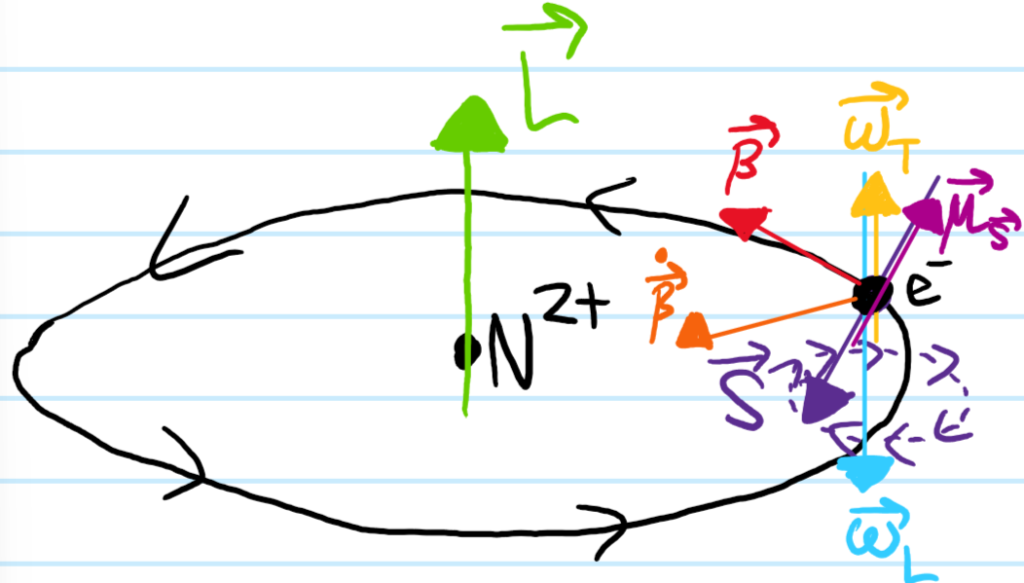
The second of these relativistic perturbations \(\Delta H_{\textbf S\cdot\textbf L}\) is the most important one of the \(3\) (especially once one moves beyond hydrogenic atoms), so it gets its own name: spin-orbit coupling. As its name suggests, it contributes a correction \(\Delta H_{\textbf S\cdot\textbf L}=\beta(|\textbf X|)\textbf S\cdot\textbf L\) proportional to the “coupling” \(\textbf S\cdot\textbf L\) of the spin angular momentum \(\textbf S\) of the electron \(e^-\) and its orbital angular momentum \(\textbf L\). The task is to determine the scalar operator of proportionality \(\beta(|\textbf X|)\) (note that \(\beta(|\textbf X|)\) commutes with both \(\textbf S\) and \(\textbf L\) by virtue of being a scalar operator, hence also commuting with \(\textbf S\cdot\textbf L\) ).
The underlying physics of spin-orbit coupling is neither particularly relativistic nor specific to quantum mechanics. In classical physics, a ball of charge \(q\) and mass \(m\) spinning with angular momentum \(\textbf S\) constitutes a current with magnetic dipole moment \(\boldsymbol{\mu}_{\textbf S}=\gamma\textbf S\) proportional to its spin angular momentum \(\textbf S\) via a proportionality constant \(\gamma=q/2m\) called its gyromagnetic ratio. When placed in an external magnetic field \(\textbf B_{\text{ext}}\), the torque \(\boldsymbol{\tau}=\boldsymbol{\mu}_{\textbf S}\times\textbf B_{\text{ext}}\) experienced by this magnetic dipole causes \(\boldsymbol{\mu}_{\textbf S}=\boldsymbol{\mu}_{\textbf S}(t)\) to precess \(\dot{\textbf S}=\boldsymbol{\omega}_L\times\textbf S\) around the axis \(\boldsymbol{\omega}_L=-\gamma\textbf B_{\text{ext}}\) at the Larmor frequency \(\omega_L=|\boldsymbol{\omega}_L|\). The dipolar potential energy \(V=-\boldsymbol{\mu}_{\textbf S}\cdot\textbf B_{\text{ext}}=\textbf S\cdot\boldsymbol{\omega}_L\) is conserved during the precession.
One should view the spin-orbit coupling of the \(e^-\) as simply taking the classical situation and appending the following relativistic and quantum mechanical paraphernalia:
The magnetic field \(\textbf B_{\text{ext}}\) is not from some external solenoid, etc. but rather due to the motion of the nucleus \(N^{Z+}\) in the rest frame of the electron \(e^-\). In light of this interpretation, a natural way to compute this magnetic field would be to just Lorentz transform the nuclear Coulomb electrostatic field \(\textbf E_{\text{ext}}=\frac{Z\alpha\hbar c}{e|\textbf X|^2}\hat{\textbf X}\) seen in the lab frame into the magnetic field \(\textbf B_{\text{ext}}=-\frac{1}{\mu c^2}\textbf P\times\textbf E_{\text{ext}}=\frac{Z\alpha\hbar}{e\mu c|\textbf X|^3}\textbf L\) seen in the rest frame of the electron \(e^-\). Alternatively, since one knows that Maxwell’s equations are Lorentz covariant, one can just work directly in the rest frame of the electron \(e^-\), using the Biot-Savart law to compute the magnetic field \(\textbf B_{\text{ext}}(\textbf 0)=\frac{\mu_0\textbf I_N}{2|\textbf X|}\) at the center of the circular current loop due to the orbit of the nucleus \(N^{Z+}\) around the electron \(e^-\) (where \(\mu\) is the reduced mass, not the magnetic dipole moment, and the nuclear current is \(\boldsymbol{\textbf I}_N=\boldsymbol{\mu}_{\textbf L}/\pi|\textbf X|^2=\gamma_{\textbf L}\textbf L/\pi|\textbf X|^2=\frac{g_{\textbf L}Ze}{2\pi m_{N}|\textbf X|^2}\textbf L_N=\frac{g_{\textbf L}Ze}{2\pi\mu|\textbf X|^2}\textbf L\)). It can be checked that these two calculations of the magnetic field \(\textbf B_{\text{ext}}\) agree with each other since \(g_{\textbf L}=1\), though both carry some classical Bohr-like handwaviness.
\(\gamma\neq q/2m\) but rather \(\gamma_{\textbf S}=g_{\textbf S}q/2m\) where \(q=-e\) and \(g_{\textbf S}\approx 2\) is the spin \(g\)-factor of the electron \(e^-\) (thus, \(\gamma_{\textbf S}<0\) and the electron’s spin and magnetic dipole moment are actually anti-aligned). The fact that \(g_{\textbf S}\neq 1\) is one of the reasons why it is often proclaimed that “spin angular momentum \(\textbf S\) has no classical counterpart” (on this note, it is a common misconception that spin is a purely quantum-mechanical effect. In fact there is no such thing as spin in non-relativistic quantum mechanics. It’s only when one combines quantum mechanicswith special relativity that spin emerges in a manner which is not merely ad hoc). Another reason is that such a literal spinning object should also have some rotational kinetic energy \(\textbf S^2/2I>0\) but classically the electron \(e^-\) is a point particle and so has \(I=0\). The effect of this to make the quantum Larmor frequency agree (almost) with the classical cyclotron frequency (some tidal-locking interpretation?).
In addition to the nuclear magnetic torque inducing the electron’s spin to precess, there is a Coriolis-like competing Thomas torque \(\boldsymbol{\tau}_T=\boldsymbol{\omega}_T\times \textbf S\) trying to make the electron spin precess in the opposite direction, except that it turns out to be only half as strong as the nuclear magnetic torque and so loses this competition (nonetheless, in the absence of such a nuclear magnetic torque, this spin precession would be called Thomas precession). This is a purely kinematic effect of special relativity due to the accumulation of Wigner rotations as one performs non-collinear Lorentz boosts from one instantaneous inertial rest frame to the next instantaneous inertial rest frame in order to “catch up with” the overall non-inertial, rotating frame of the electron \(e^-\). Within the Lorentz group \(O(1,3)\), the Lorentz boosts by themselves do not form a subgroup of \(O(1,3)\) but when combined with spatial rotations, this does form a subgroup, since:
where it is obvious that \(\gamma_3=\gamma_1\gamma_2(1+\boldsymbol{\beta}_1\cdot\boldsymbol{\beta}_2)\) and by taking the trace \(\text{Tr}(R)=1+2\cos\theta\) of \(R\in SO(3)\), one finds that it is associated to a Wigner rotation angle \(\cos\theta=\frac{(1+\gamma_1+\gamma_2+\gamma_3)^2}{(1+\gamma_1)(1+\gamma_2)(1+\gamma_3)}-1\). In particular, when \(\boldsymbol{\beta}_1\cdot\boldsymbol{\beta}_2=0\) are orthogonal as in “circular motion” of the electron \(e^-\) around the nucleus, then \(\gamma_3=\gamma_1\gamma_2\) and the Wigner rotation simplifies to \(\cos\theta=\frac{\gamma_1+\gamma_2}{\gamma_1\gamma_2+1}\). In particular, taking \(\gamma_1=\gamma_{\boldsymbol{\beta}}\) and Taylor expanding \(\gamma_2=\gamma_{\boldsymbol{\beta}+d\boldsymbol{\beta}}\approx\gamma_{\boldsymbol{\beta}}+\gamma_{\boldsymbol{\beta}}^3\boldsymbol{\beta}\cdot d\boldsymbol{\beta}\), one can use the generators of the Lie algebra of the subgroup of \(O(1,3)\) consisting of Lorentz boosts + rotations to show that the Thomas precession angular velocity is (notice the prefactor \(\frac{\gamma^2}{\gamma+1}\) is the same expression appearing in the Lorentz boost matrix):
The factor of \(1/2\) is called the Thomas half and cancels out essentially half of the spin-orbit coupling Larmor precession. This is because one just has to replace the previous Larmor frequency with \(\boldsymbol{\omega}_L\mapsto\boldsymbol{\omega}_L+\boldsymbol{\omega}_T\), noting that “Larmor is twice as strong as Thomas” \(\boldsymbol{\omega}_T\approx -\boldsymbol{\omega}_L/2\) (apply Newton’s second law \(\mu\dot{\boldsymbol{\beta}}=-ec\textbf E_{\text{ext}}\) and use the earlier formula for the Lorentz transformation of the nuclear Coulomb electrostatic field \(\textbf E_{\text{ext}}\) into the magnetic field \(\textbf B_{\text{ext}}\)).
Assembling all the ingredients together, one finds the relativistic spin-orbit coupling perturbation to be given by \(\Delta H_{\textbf S\cdot\textbf L}=\beta(|\textbf X|)\textbf S\cdot\textbf L\) as claimed, where the scalar proportionality operator \(\beta(|\textbf X|)=\frac{Z\alpha\hbar(g_{\textbf S}-1)}{2\mu^2c|\textbf X|^3}>0\) is positive-definite so if the electron \(e^-\) is orbiting counterclockwise around the nucleus \(N^{Z+}\), then it will tend to spin clockwise to minimize its spin-orbit coupling energy \(\beta(|\textbf X|)\textbf S\cdot\textbf L\). A picture is worth a thousand words (analogy: the spin angular momentum vector \(\textbf S\) is like a cylinder rolling on a cone).
One can check that \(\textbf S\cdot\textbf L=\frac{1}{2}(S_+L_-+S_-L_+)+S_3L_3\). By observing that the only surviving combinations of ladder operators are \(S_{\pm}L_{\mp}\) and not \(S_+L_+\) or \(S_-L_-\), one is led to the heuristic that if the electron \(e^-\) gains a unit \(\hbar\) of orbital angular momentum \(L_3\) along the \(z\)-axis, then it must lose a unit \(\hbar\) of spin angular momentum \(S_3\) along the \(z\)-axis, and vice versa, in such a way that the total angular momentum \(J_3=L_3+S_3\) along the \(z\)-axis is conserved. To this end, one can regard \(J_3\) as the \(z\)-component of a total angular momentum operator \(\textbf J:=\textbf L+\textbf S\) so that \(\textbf S\cdot\textbf L=\frac{1}{2}(\textbf J^2-\textbf L^2-\textbf S^2)\). In particular, \([H,\textbf J^2]=[H,J_3]=0\) so working in the coupled basis \(|njm_j;\ell s\rangle\) rather than the previously uncoupled basis \(|n\ell sm_{\ell}m_s\rangle\) yields:
using the fact that the electron is a spin \(s=1/2\) fermion and so by the usual rules of angular momentum addition one has \(m_j=m_{\ell}+m_s\) and \(|\ell-s|\leq j\leq \ell+s\) which is equivalent to \(j=\ell\pm 1/2\) (except for \(\ell=0\) \(s\)-waves where \(j=1/2\) only), this simplifies to:
In other words, when the orbital and spin angular momenta are aligned \(j=\ell+1/2\), the spin-orbit coupling energy is \(\sim\hbar^2\ell/2\) whereas when the orbital and spin angular momenta are anti-aligned \(j=\ell-1/2\), then the energy is \(\sim-\hbar^2(\ell+1)/2\), in agreement with the earlier intuition about the anti-aligned configuration being more energetically favorable. In particular, for \(\ell=0\) \(s\)-waves where only the case \(j=1/2\) is relevant, the spin-orbit coupling energy evaluates to \(\hbar^2\times 0/2=0\) so spin-orbit coupling does not affect the ground state(s) \(|100,\pm 1/2\rangle\).
Relativistic Darwin Perturbation
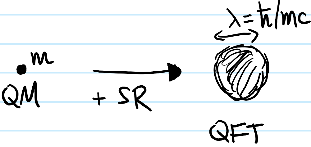
One of the key corollaries of merging special relativity and quantum mechanics is that all the “particles” one is used to such as protons, electrons, etc. are not in fact point particles but rather are smeared out clouds of size \(\lambda\):
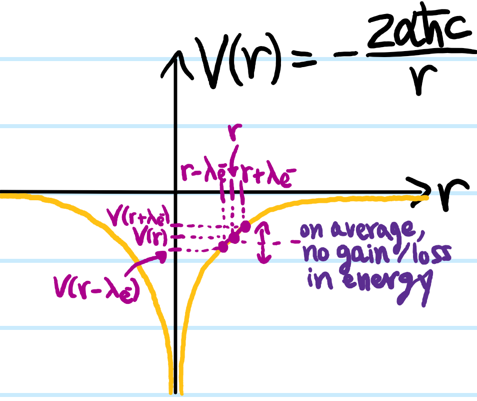
where \(\lambda=\hbar/mc\) is the Compton wavelength of the particle of mass \(m\). Thus for instance, photons \(\gamma\) with \(m_{\gamma}=0\) have \(\lambda_{\gamma}=\infty\) whereas an electron \(e^-\) (which is what one is interested in here) has \(m_{e^-}\sim 10^{-30}\text{ kg}\) and so \(\lambda_{e^-}\sim 10^{-34}/(10^{-30}\times 10^8)\text{ m}\sim 10^{-12}\text{ m}\) (the exact Compton wavelength turns out to be \(\lambda_{e^-}\approx 2.43\times 10^{-12}\text{ m}\)). On these picometer length scales, the electron \(e^-\) no longer looks like a point but rather a swarm of particles and antiparticles. Compared with the Bohr radius \(a_0\approx\lambda_{e^-}/\alpha\), these rapid quantum oscillations (“Zitterbewegung“) are still quite tiny. Consequently, the potential energy of the nucleus \(N^{Z+}\) (which technically also has some nuclear Compton wavelength \(\lambda_N=\lambda_{e^-}\mu/m_N\) except its even shorter than that of the electron \(e^-\) by a factor of \(\mu/m_N\sim 1/1836\), so it is safe to model the nucleus \(N^{Z+}\) as still being a point charge) and the electron \(e^-\) will basically be the same whether one thinks of the electron \(e^-\) as a point charge or as a \(\lambda_{e^-}\)-ball. In the latter case, one roughly expects the electron \(e^-\) to be a distance \(\lambda_{e^-}\) closer to the nucleus \(N^{Z+}\) sometimes, hence experiencing a slightly stronger potential energy \(\sim V(r-\lambda_{e^-})\), but at other times a distance \(\lambda_{e^-}\) further away, experiencing a slightly weaker potential \(\sim V(r+\lambda_{e^-})\) so that heuristically one expects this to just average to \(\sim V(r)\):
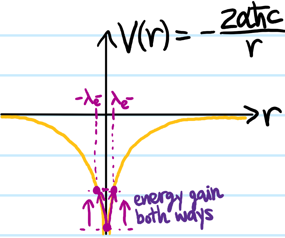
However, there is one point on the diagram where this heuristic clearly fails, namely at the origin \(r=0\) where the nucleus \(N^{Z+}\) rests; here, no matter which direction \(\pm\lambda_{e^-}\) the electron \(e^-\) oscillates, its potential energy \(V(\pm\lambda_{e^-})>V(0)\) can only increase because \(r=0\) is a (global) minimum of the Coulomb potential \(V(r)\) (of course, these arguments are a bit handwavy because \(V(r)\) is actually undefined at \(r=0\)):
Combined with the fact that Coulomb potential is steepest at \(r=0\), this suggests that only states which can approach the origin \(r=0\) would notice anything. In other words, \(\ell=0\) \(s\)-waves! To formalize this intuition, one can explicitly compute the average Coulomb potential \(\langle V(\textbf x)\rangle_{\lambda_{e^-}}\) in a \(\lambda_{e^-}\)-ball at some position \(\textbf x\in\textbf R^3\):
one sees that the zeroth-order term \(V(\textbf x)\) averages to itself, being just the nuclear Coulomb potential that was in the gross structure Hamiltonian \(H_{\text{gross}}\) all along. The first-order term \(d\textbf x\cdot\frac{\partial V}{\partial\textbf x}\) vanishes upon isotropic averaging. However, the second-order term does not necessarily vanish. It is the averaging of this second-order term which should therefore be treated as the relativistic Darwin perturbation \(\Delta H_{\text{Darwin}}=\frac{1}{2}\langle d\textbf x\cdot\frac{\partial^2 V}{\partial\textbf x^2}d\textbf x\rangle_{\lambda_{e^-}}=\frac{1}{2}\partial_{\mu}\partial_{\nu}V\langle dx^{\mu}dx^{\nu}\rangle_{\lambda_{e^-}}\). For distinct directions \(\mu\neq\nu\) one expects these fluctuations to be uncorrelated, whereas along a given axis \(\mu=\nu\), dimensional analysis asserts that the variance must be of order \(\lambda_{e^-}^2\). However, the exact proportionality constant is not so easy to figure out; a calculation using the Dirac equation shows that the covariance matrix is diagonal with:
By virtue of the Dirac delta operator \(\delta^3(\textbf X)\), the relativistic Darwin perturbation only affects states which can approach the origin \(r=0\), again suggesting it only affects \(\ell=0\) \(s\)-waves. This is to be contrasted with spin-orbit coupling which affected all states except for \(\ell=0\) \(s\)-waves.
Fine Structure Corrections to Gross Structure Energies
Having reasoned from physics first principles to derive the relativistic perturbation Hamiltonian:
the task now becomes to calculate how the degeneracy in the gross structure energies \(E_n\) is lifted by these relativistic perturbations \(\Delta H_{\text{SR}}\) to yield the fine structure of the hydrogenic atom. As usual, the eigenspaces of the gross structure Hamiltonian \(H_{\text{gross}}\) are labelled by principal quantum number \(n\in\textbf Z^+\) and have \(2n^2\)-degeneracy as mentioned earlier, so a priori one has to use degenerate perturbation theory. This means one needs to evaluate the matrix elements of \(\Delta H_{\text{SR}}\) restricted to each energy eigenspace \(\ker(H_{\text{gross}}-E_n1)\). Here, the important thing is to choose the right basis for \(\ker(H_{\text{gross}}-E_n1)\) with respect to which one would be calculating the matrix elements of the perturbation \(\Delta H_{\text{SR}}\). Ideally, one would somehow correctly guess an eigenbasis for \(\Delta H_{\text{SR}}\) so that the matrix elements would be trivial to evaluate (all off-diagonal matrix elements would vanish, leaving only expectations on the diagonal so that the different states don’t mix and one is effectively doing non-degenerate perturbation theory). Note that the Wigner-Eckart theorem is useless here because it is not clear how \(\Delta H_{\text{SR}}\) can be interpreted as a component of some spherical tensor operator in the spherical basis. Instead, the idea is contained in the following lemma:
Lemma: Let \(A\) be a Hermitian operator with eigenstates \(|\alpha\rangle, |\alpha’\rangle\) corresponding to distinct eigenvalues \(\alpha\neq\alpha’\in\textbf R\) (hence \(\langle\alpha’|\alpha\rangle=0\)). Suppose that \(A\) commutes with an arbitrary (not necessarily Hermitian) operator \(\Delta H\), i.e. \([A,\Delta H]=0\). Then the off-diagonal matrix element \(\langle\alpha’|\Delta H|\alpha\rangle=0\) vanishes.
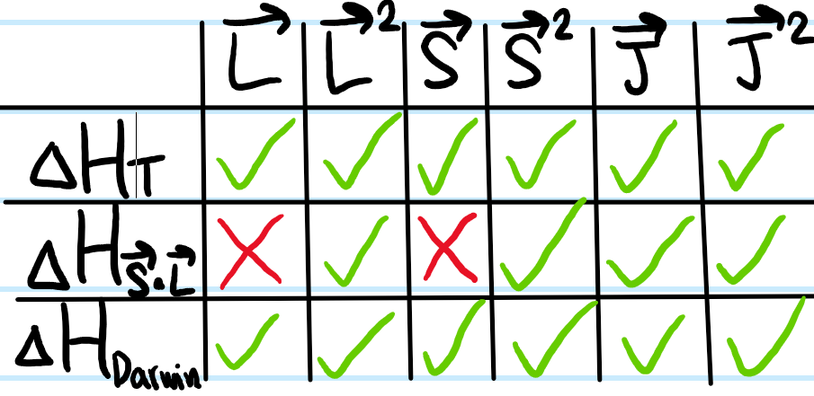
Thus, here the idea is that one would like to find a complete set of commuting observables (i.e. a set of pairwise-commuting observables with unique simultaneous eigenbasis for the entire state space \(\mathcal H\)) such that as many of the observables in this CSCO also commute with the relativistic perturbation \(\Delta H_{\text{SR}}\). In this case, one can quickly check that:
where the green check mark means the two operators commute, the red x if not. It is clear in this case that the CSCO to use is \(\{\textbf L^2,\textbf S^2,\textbf J,\textbf J^2\}\). But this is just the coupled basis \(|njm_j;\ell s\rangle\) mentioned earlier. Working in the uncoupled basis \(|n\ell sm_{\ell}m_s\rangle\) is fine for \(\Delta H_T\) and \(\Delta H_{\text{Darwin}}\) but spin-orbit coupling \(\Delta H_{\textbf S\cdot\textbf L}\) doesn’t like that. Working in the coupled basis makes everyone happy. Degenerate perturbation theory thus reduces to non-degenerate perturbation theory since the coupled basis states don’t mix.
The expectation \(\langle njm_j;\ell s|\Delta H_T|njm_j;\ell s\rangle\) of the relativistic kinetic energy perturbation \(\Delta H_T\) is actually most easily calculated by using Clebsch-Gordan coefficients to rotate back into the uncoupled basis (simply using the resolution of the identity \(|njm_j;\ell s\rangle=\sum_{m_{\ell}m_s}|n\ell sm_{\ell}m_s\rangle\langle\ell sm_{\ell}m_s|jm_j\rangle\) for the ket and similarly for the bra. Note here that the \(s=1/2\) quantum number is being explicitly shown but in practice is often suppressed in the notation because it’s a constant):
Since \([\Delta H_T,\textbf L]=[\Delta H_T,\textbf S]=0\) (e.g. see the table above), this means \(\Delta H_T\) is a scalar (rank \(0\)) operator with respect to both orbital and spin angular momenta and so by the Wigner-Eckart theorem:
\[\langle n\ell sm_{\ell}’m_s’|\Delta H_T|n\ell sm_{\ell}m_s\rangle=\delta_{m_{\ell}m_{\ell}’}\delta_{m_{s}m_{s}’}\langle n\ell s 0,1/2|\Delta H_T|n\ell s 0,1/2\rangle\]
where the values \(m_{\ell}=0, m_s=1/2\) are arbitrarily chosen for the reduced matrix element (since it doesn’t matter). The computation thus simplifies significantly by virtue of orthonormality \(\sum_{m_{\ell},m_s}\langle j’m_j’|\ell sm_{\ell}m_s\rangle\langle\ell sm_{\ell}m_s|jm_j\rangle=\delta_{jj’}\delta_{m_jm_j’}\) of Clebsch-Gordan coefficients (where here \(j’=j\) and \(m_j’=m_j\)):
\[\langle njm_j;\ell|\Delta H_T|njm_j;\ell\rangle=\langle n\ell s 0,1/2|\Delta H_T|n\ell s 0,1/2\rangle\]
Finally, evaluating the orbital matrix element:
\[\langle n\ell s 0,1/2|\Delta H_T|n\ell s 0,1/2\rangle=-\frac{1}{2\mu c^2}\biggr\langle n\ell s 0,1/2\biggr|\left(\frac{\textbf P^2}{2\mu}\right)^2\biggr|n\ell s 0,1/2\biggr\rangle\]
By writing \(\frac{\textbf P^2}{2\mu}=H_{\text{gross}}-V\), this simplifies to:
\[\langle n\ell s 0,1/2|\Delta H_T|n\ell s 0,1/2\rangle=-\frac{1}{2\mu c^2}(E_n^2-2E_n\langle V\rangle_{n,\ell}+\langle V^2\rangle_{n,\ell})\]
The expectation \(\langle V\rangle_{n,\ell}=2\langle H_{\text{gross}}\rangle_{n,\ell}=2E_n\) is trivial by the virial theorem. However, the expectation \(\langle V^2\rangle_{n,\ell}\) is not so trivial, and requires some mathematical cleverness to evaluate. It turns out to be (and in the circular Rydberg limit \(n\gg 1\), \(\ell=n-1\), agrees with the Bohr model):
Thus, assembling everything together, the first-order correction to the gross structure energies due to the relativistic kinetic energy perturbation \(\Delta H_T\) alone is:
\[\langle n\ell s 0,1/2|\Delta H_T|n\ell s 0,1/2\rangle=-\frac{1}{2}\left(\frac{Z\alpha}{n}\right)^4\left(\frac{n}{\ell+1/2}-\frac{3}{4}\right)\mu c^2<0\]
Now onto spin-orbit coupling. One has (following similar Clebsch-Gordan coefficient manipulations as above and using the earlier results):
Here another bit of mathematical cleverness (using the scalar radial momentum operator \(P_r:=(\hat{\textbf X}\cdot\textbf P+\textbf P\cdot\hat{\textbf X})/2\) to derive the Kramers-Pasternack recurrence relations) is needed to show that:
Finally, for the relativistic Darwin term, using the same kinds of arguments as above, one finds (using \(\langle\textbf 0|n\ell sm_{\ell}m_s\rangle=\frac{2}{\sqrt{4\pi}}\left(\frac{Z}{na_0}\right)^{3/2}\delta_{\ell,0}\)) that:
there are \(2\) miracles that have happened here. The first is that, for \(\ell>0\), the above formula is the result one would obtain regardless of whether \(j=\ell\pm 1/2\) (an accidental degeneracy in this context, though actually natural if one starts from the Dirac equation). The second miracle is that, when \(\ell=0\), the spin-orbit coupling correction should actually vanish, but then the Darwin correction kicks in and adds back exactly what spin-orbit coupling would have added, so that the final formula is valid for all \(\ell\in\textbf N\) and \(j=\ell\pm 1/2\) (remembering that for \(\ell=0\) one only has \(j=1/2\)). This should be compared with the “exact” expression at the level of fine structure given by the Dirac equation:
Thus, at a high level, after spin-orbit coupling was introduced, \(m_{\ell},m_s\) were no longer good quantum numbers (but \(n,\ell,s\) still were), so had to be replaced by two new good quantum numbers \(j,m_j\). These fine structure corrections actually failed to lift the \(\ell\)-degeneracy, but nevertheless there is now a \(j\)-dependence which wasn’t there at the level of the gross structure.
Comments about notation \(n\ell_j\) and degeneracy of states in \(n\ell_j=\sum_{j=\ell\pm 1/2}(2j+1)\)?
Hyperfine Structure of Hydrogenic Atoms
Just as the fine structure of hydrogenic atoms was obtained from special relativity, one could roughly say that the hyperfine structure of hydrogenic atoms comes from quantum chromodynamics, or more simply, from no longer treating the nucleus \(N^{Z+}\) as just a point charge \(Ze\) at the origin, but rather having some internal structure to it as well. In other words, it turns out (because protons \(p^+\) and neutrons \(n^0\) are spin-\(1/2\) fermions just like the electron \(e^-\)) that the nucleus \(N^{Z+}\) also has some spin angular momentum \(\textbf I:=\textbf S_{N}\) which gives rise to a nuclear magnetic dipole moment \(\boldsymbol{\mu}_{\textbf I}=\gamma_{\textbf I}\textbf I\) where now the nuclear gyromagnetic ratio is \(\gamma_{\textbf I}=\frac{g_{\textbf I}Ze}{2m_N}\). There are \(2\) other angular momenta that the nuclear spin angular momentum \(\textbf I\) can couple to, namely the orbital angular momentum \(\textbf L\) of the electron \(e^-\) and its spin angular momentum \(\textbf S\). These lead respectively to nuclear perturbations \(\Delta H_N=\Delta H_{\textbf I\cdot\textbf L}+\Delta H_{\textbf I\cdot\textbf S}\) to the fine structure Hamiltonian \(H_{\text{HFS}}=H_{\text{FS}}+\Delta H_N\) given respectively by:
The former is just spin-orbit coupling but now in the rest frame of the nucleus (which is normally one how thinks about hydrogenic atoms anyways). The second is just the standard formula from electromagnetism for the interaction energy between two dipoles due to their intrinsic magnetic fields. Although normally one wouldn’t really care about the \(\delta^3(\textbf X)\) term since one is typically interested in the far-field behavior of the magnetic field, actually here it turns out to be crucial! Finally, note that sometimes the electric quadrupole moment (NOT a magnetic quadrupole moment) of the nucleus \(N^{Z+}\) and its interaction with the non-uniformelectric (not magnetic!) field of the electron \(e^-\) is also counted as a hyperfine effect, but here it will just be ignored.
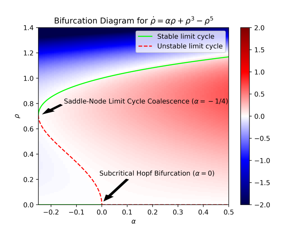
Consider the following \(2\)D dynamical system expressed in plane polar coordinates \((\rho,\phi)\):
\[\dot{\rho}=\alpha\rho+\rho^3-\rho^5\]
\[\dot{\phi}=\omega+\beta\rho^2\]
with \(3\) real parameters \(\alpha,\omega,\beta\in\textbf R\). Since \(\rho\) is decoupled from \(\phi\) (but not vice versa) one can analyze \(\rho\) on its own. A simple calculation shows that nullclines \(\dot{\rho}=0\) are circular limit cycles in phase space at radii \(\rho=0\) (the origin) and \(\rho_{\pm}=\sqrt{\frac{1\pm\sqrt{1+4\alpha}}{2}}\). These yield the following bifurcation diagram for the dynamical system:
And here is an animation of the above situation in the phase plane (with the color again indicating the value of \(\dot{\rho}\)) letting the parameter \(\alpha\) increase from \(\alpha=-0.3\) to \(\alpha=0.1\). The saddle-node limit cycle coalescence at \(\alpha=-0.25\) is evident, as a half-stable limit cycle seemingly materializes out of thin air at \(\rho=1/\sqrt{2}\) and then bifurcates into the stable limit cycle \(\rho_+=\sqrt{\frac{1+\sqrt{1+4\alpha}}{2}}\) and an unstable limit cycle \(\rho_-=\sqrt{\frac{1-\sqrt{1+4\alpha}}{2}}\) that move apart from each other for \(\alpha\in(-0.25,0)\). Then at \(\alpha=0\), the unstable limit cycle chokes the attracting fixed point at the origin, undergoing a subcritical Hopf bifurcation such that for \(\alpha>0\) the origin becomes a repelling fixed point and the remaining stable limit cycle from earlier “sucks” all trajectories onto it.
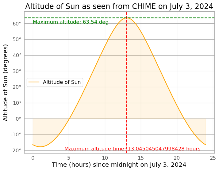
As a \(2024\) summer intern in the University of Toronto’s Summer Undergraduate Research Program, I will be working with Dr. Nina Gusinskaia and Dr. Rik van Lieshout (both postdoctoral researchers working jointly at the Canadian Institute for Theoretical Astrophysics (CITA) and the Dunlap Institute for Astronomy & Astrophysics) in the University of Toronto Radio Astronomy and InstrumentatioN Lab (UTRAINLab) headed by Professor Juan Mena-Parra to conduct detailed observational studies of fast radio bursts (FRBs), pulsarscintillometry, and radio interferometry. The purpose of this post is to document my learning journey over the summer with regards to this endeavor. One particularly exciting aspect about this project is that a lot of the pipelines for calibration that I develop can be used eventually for actual projects such as outrigger stations being commissioned in California or BURSTT/KKO projects in Taiwan.
Pulsars
At an astronomy level, a pulsar is just a rotating neutron star (which itself is a misnomer since it’s not really a “star” but actually it’s the corpse of what used to be a fairly massive star! In other words, neutron stars are dead stars). By contrast, at a physics level, a pulsar is a rotating magnetic dipole where in general \(\boldsymbol{\omega}\) and \(\boldsymbol{\mu}\) are not necessarily aligned, giving pulsars their nickname as “cosmic lighthouses”. The magnetic field looks qualitatively like the usual magnetic dipole field \(\textbf B(\textbf x)=\frac{\mu_0}{4\pi}\left(\frac{3(\boldsymbol{\mu}\cdot\hat{\textbf x})\hat{\textbf x}-\boldsymbol{\mu}}{|\textbf x|^3}\right)\). The pulsar’s radius \(R\), density \(\rho\), wavelength \(\lambda\) of emission, and polarization \(\textbf E\) of the light, etc. are all also important parameters to keep in mind.
Pulsars provide a wealth of information about neutron star physics, general relativity, the galactic gravitational potential \(\phi_g(\textbf x,t)\), the galactic magnetic field \(\textbf B_g(\textbf x,t)\), the galactic charge density \(\rho_e(\textbf x,t)\), and more generally many properties (i.e. fields defined on) of the interstellar medium (ISM).
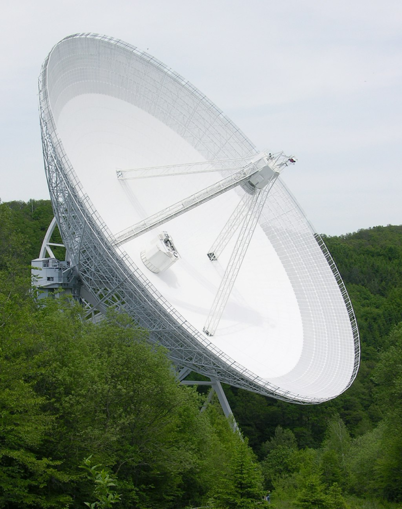
Experimentally, pulsar research is driven by surveys of the cosmos with large radio telescopes (a bit of a misnomer, since it’s not really a “telescope” in the traditional sense of an optical telescope) which are typically parabolic antennas (“dishes”) like the one below designed to focus radio waves:
The 100 meter Effelsberg radio telescope, in Bad Münstereifel, Germany
With such large radio telescopes, one challenge is to build them without deformation under their own weight (which would ruin for instance their parabolic surface). A variety of ingenious ways have been devised to solve that problem.
The nomenclature convention for pulsars is to start with “PSR”, followed by “B” or “J” depending on whether it was discovered before or after \(1990\), and then the celestial coordinates of the pulsar.
All binary pulsar systems will eventually coalesce in the limit \(t\to\infty\) due to energy loss via gravitational wave emission.
The pulsar PSR B1937+21 rotates at \(f_{\text{PSR}}=642\text{ Hz}\), which is quite close to the theoretical limit frequency of rotation \(f_{\text{PSR}}^*\).
Pulsars have also been found in globular clusters, with exoplanetary systems, triple systems, and even double pulsars.
Most pulsars to date have been found by the Parkes radio telescope in Australia. Although pulsar astronomy does involve probing across the electromagnetic spectrum, the most important wavelengths are radio.
On a radio telescope antenna, pulsar radio waves are received as “spikes” in the irradiance profile \(I(t)\) received. This irradiance is not in general monochromatic however, but rather is distributed over all frequencies according to \(I=\int_0^{\infty}\rho_I(f)df\) for some spectral irradiance density with respect to frequency \(\rho_I(f)\) measured typically in janskys \(1\text{ Jy}:=10^{-26}\frac{\text W}{\text m^2\cdot\text{Hz}}\). For most pulsars, the spectral irradiance density with respect to frequency is concentrated at low \(f\) (e.g. radio waves). When plotting \(\log(\rho_I(f))\) against \(\log(f)\), one tends to observe a linear decrease in the high-frequency regime \(\log(f)\gg 1\), suggesting a power law dependence of the form \(\rho_I(f)\propto f^{\alpha}\) where \(\alpha<0\) is the spectral index of the pulsar.
In general, if one views the pulsar rotation period \(T_{\text{PSR}}\) as a continuous random variable, then the probability density function \(\rho_{T_{\text{PSR}}}\) of \(T_{\text{PSR}}\) is bimodal, with one hump representing short-period, millisecond pulsars which are more ancient and the other hump representing long-period, younger pulsars with a different evolutionary history. Thus, one seems to find a Heisenberg correlation between time of formation \(\Delta_f t\) and rotation period \(T_{\text{PSR}}\).
Individual pulses from pulsars are very weak radio sources (can only see individual pulses for the “brightest” pulsars). Furthermore, individual pulses turn out to be highly variable due to both stochastic noise and systematic effects (e.g. periodic intensity modulation, drifting sub-pulses, mode changing, nulling, etc.) but if one performs an averaging procedure to obtain a so-called integrated pulse profile \(\bar I(t)\), then, in analogy to the central limit theorem from statistics, one has:
Fundamental “Theorem” of Pulsar Astronomy: the integrated pulse profile \(\bar I(t)\) is stable for \(t\in\textbf R\).
Since pulsars tend to be very polarized, a well-calibrated polarimeter can offer accurate determination of \(4\) Stokes parameters \(S_0,S_1,S_2,S_3\) which can be combined into a Stokes vector \(\textbf S:=(S_0,S_1,S_2,S_3)^T\in\textbf R^4\). The precise definitions of each the \(S_i\) is in terms of certain electric field components, though in essence the Stokes vector provides a bijection with all possible elliptic polarization of light from the pulsar. As this polarized light propagates through the ISM, it also undergoes Faraday rotation due to the galactic magnetic field \(\textbf B_g\) with the spatial rate \(\frac{\partial\theta}{\partial x}\) of such Faraday rotation being proportional to \(\textbf B_g\cdot\textbf k\) where \(\textbf k\) is the angular wavevector and the constant of proportionality is called the Verdet constant.
By applying a simple harmonic oscillator model to the ISM as an electron plasma, one can show that the time \(\Delta t\) required for light of frequency \(f\) to reach Earth from a pulsar a distance \(d\) away is:
where the line integral \(\int_0^dn_{e^-}d\ell\) is taken along the line of sight between the pulsar and Earth and is called the dispersion measure of the pulsar since it determines the degree to which the interstellar medium optically disperses the various frequencies of light from the pulsar (units of the dispersion measure are typically \(\text{pc}/\text{cm}^3\)). This can be used to map out the \(e^-\) density of the galaxy.
Contrary to what one might intuitively expect, the interstellar medium is actually a turbulent and non-uniform fluid (more precisely an electron plasma). This is directly responsible for a sort of interstellar scintillation effect (analogous to how turbulence in the atmosphere causes star light to twinkle, except here the scintillation/twinkling effect is for radio waves rather than visible light). Quantitatively, one can adapt a very simple thin screen model to model the interstellar medium, one prediction of which is that interstellar scintillation broadens the frequency spectrum by some scintillation bandwidth \(\Delta f\) which is proportional to \(f^4\) (where \(f\) is the observing frequency). This manifests as an exponential tail in plots of \(I(t)\) for folded pulsar signals, where the time scale \(\tau_s\propto\frac{1}{\Delta f}\propto\frac{1}{f^4}\) of such an exponential decay is called the scattering time and in the thin-screen model is explained by variations in mean free path. Obviously, a larger \(\tau_s\) is undesirable because it implies a broader pulse, hence a lower SNR. This means that radio telescopes generally should observe at higher \(f\) (e.g. the Parkes radio telescope’s multibeam galactic plane survey at \(f=1.4\text{ GHz}\) discovered much more dispersed and scattered pulsars than previous low-\(f\) surveys (although actually observing is never at a single frequency \(f\), but rather in some bandwidth of frequencies \([f-\Delta f/2,f+\Delta f/2]\).
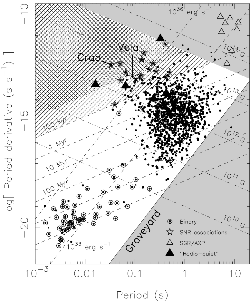
Finally, a bit about the population statistics of pulsars. Most, by observational bias, have been found in the Milky Way’s galactic plane and in particular near our Solar System. As pulsars emit radiation (rotating magnetic dipoles!), they lose rotational kinetic energy. As this energy drops, therefore their rotational period \(T\) increases \(\dot T>0\). In general, both \(T\) and \(\dot T\) can be obtained precisely via timing measurements. Therefore, if one plots \(\log(T)\) vs. \(\log(\dot T)\), one finds a clear separation of pulsars into “normal” pulsars in the upper right quadrant and millisecond pulsars in the bottom left.
It can be shown from a simple rotating magnetic dipole model that:
\[t_{\text{age}}\propto\frac{T}{\dot T}\]
\[B\propto\sqrt{T\dot T}\]
\[\dot E\propto\frac{\dot T}{T^3}\]
Quite naturally, this data suggests that pulsars begin as “normal” pulsars and then at some point rapidly spin down into the millisecond pulsars domain (the rapid nature of this spin down process would explain why there are no pulsars intermediate). It is also interesting to note that most binary pulsars (not necessarily \(2\) pulsars orbiting each other but just a pulsar orbiting another celestial object) are in the millisecond pulsars category).
Antenna Fundamentals
Roughly speaking, in the lingo of particle physics, an antenna is any conductor that mediates interactions between photons \(\gamma\) and electrons \(e^-\). That is:
\[\gamma\leftrightarrow e^-\]
More precisely, thinking of photons \(\gamma\) in the classical way as propagating electromagnetic \((\textbf E,\textbf B)\) waves, an antenna can be used either as a transmitting antenna meaning that an external driving voltage source \(V\) (called a transmitter and which needs to be impedance-matched \(Z_{\text{transmitter}}=Z_{\text{antenna}}^{\dagger}\) with the antenna via an antenna tuner circuit to maximize power delivery to the antenna rather than allow the power to “reflect” from the antenna back to the transmitter and form standing waves) induces a corresponding AC current \(I=V/Z_{\text{antenna}}\) in the antenna so that accelerating electrons \(e^-\) will emit electromagnetic radiation (photons \(\gamma\)); thus for a transmitting antenna one has \(e^-\to\gamma\). By contrast, the same antenna can also be used as a receiving antenna so external electromagnetic waves (e.g. from celestial sources, terrestrial interference, etc.) exert a Lorentz force \(\textbf f=\rho\textbf E+\textbf J\times\textbf B\) on the electrons \(e^-\) in the antenna, causing them to slosh into an AC current \(I\) (which is then recorded by an impedance-matched receiver unit); thus for a receiving antenna \(\gamma\to e^-\).
As one might expect, transmitting antennas might transmit EM radiation better in some directions \(\hat{\textbf n}\) than others, and similarly receiving antennas may be more sensitive to EM radiation coming from some directions \(\hat{\textbf n}\) than others. This is quantified by the directivity of the antenna \(D:S^2\to[0,\infty)\) which maps each direction \(\hat{\textbf n}\in S^2\) on the celestial sphere \(S^2\) to a dimensionless non-negative real number \(D(\hat{\textbf n})\geq 0\) describing how “directed” the antenna is in that direction \(\hat{\textbf n}\):
where \(\hat P\) is the power per unit solid angle (SI units: \(\text W/\text{sr}\)) on \(S^2\) so that the total power of the entire sky would be given by \(P=\iint_{\hat{\textbf n}\in S^2}\hat P(\hat{\textbf n})d^2\hat{\textbf n}\) and \(\overline{\hat P}=P/4\pi\) is the average power per unit solid angle.
The maximum directivity \(D^*\in [1,\infty)\) (also just called the directivity if no direction \(\hat{\textbf n}\) is specified) is simply:
and is usually expressed in decibels \(D^*_{\text{dBi}}=10\log(D^*)\). For instance, an (idealized, theoretical, not-actually-a-thing) isotropic antenna by definition exhibits an isotropic power profile \(\hat P(\hat{\textbf n})=P_0\) for some constant \(P_0\) across the sky \(S^2\) so that it also exhibits an isotropic directivity \(D(\hat{\textbf n})=1\) and correspondingly \(D^*=1\) or \(D^*_{\text{dB}}=0\text{ dBi}\) (the minimum possible maximum directivity!). This explains why the logarithmic form \(D^*\) has decibel units called “dBi” since the “i” stands for “isotropic”, implying that the decibel comparison is with the isotropic antenna \(D^*_{\text{dBi}}=10\log(D^*)=10\log(D^*/1)\).
One might worry that there should be a need to distinguish between \(D_{\text{transmitting}}\) and \(D_{\text{receiving}}\), i.e. that the antenna may have different directivities depending on whether it’s being used as a transmitting antenna or a receiving antenna. Fortunately, a deep symmetry of Maxwell’s equations known as electromagnetic reciprocity guarantees, among other corollaries, that the transmitting and receiving directivities for any antenna are identical, i.e.
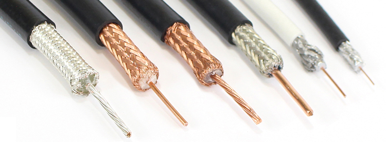
(more precisely, electromagnetic reciprocity holds for passive antennas, not for active antennas). However, in practice the directivity isn’t the only factor that one cares about; there is also the transmission line (often coaxial cable for radio applications) between the antennas and transmitter/receiver units so that one is not just interested in the directivity \(D(\hat{\textbf n})\) of the antenna but also its gain \(G(\hat{\textbf n})\in [0,\infty)\), which is proportional to its directivity \(G(\hat{\textbf n}):=\eta D(\hat{\textbf n})\) where the constant of proportionality \(\eta\in[0,1]\) is called the radiation efficiency and is defined in the obvious manner by the ratio:
More precisely, for a transmitting antenna, \(\eta=P_{\text{antenna}\to S^2}/P_{\text{transmitter}\to\text{antenna}}\) whereas for a receiving antenna, \(\eta=P_{\text{antenna}\to\text{receiver}}/P_{S^2\to\text{antenna}}\). Combining with the previous definition of directivity (where the notation \(P\) was used for what is being denoted by \(P_{\text{output}}\) above), one can also write \(G(\hat{\textbf n})=4\pi\hat{P}(\hat{\textbf n})/P_{\text{input}}\). Finally, it is also common to speak of the maximum gain \(G^*:=\eta D^*\) (or just gain if no direction is given) and as with directivities, it is conventional to express gains logarithmically \(G_{dBi}:=10\log(G)\).
One common way of studying an antenna is to plot its gain profile \(G(\hat{\textbf n})\) (or some planar cross-section thereof) in polar coordinates. For instance,
Radio Interferometry
There are several benefits enjoyed by radio astronomy which are not enjoyed by optical astronomy.
To start, it suffices to consider the case of cross-correlating just \(N=2\) radio telescopes, since a more general array of \(N\) radio telescopes is equivalent to \(\frac{N(N-1)}{2}\) pairs of radio telescopes, thus growing quadratically in \(N\) (e.g. the Atacama Large Millimeter/Submillimeter Array (ALMA) in Chile boasts \(N=66\) radio telescopes, yielding a total of \(2145\) pairs of radio telescopes).
The (complex) visibility \(V(u,v)\) is defined to be … it is then a non-trivial result of optical coherence theory known as the van Cittert-Zernike theorem (intuitively, the geometric effect that a sum of incoherent waves will become more spatially coherent with propagation distance). that the complex visibility is also the Fourier transform of the spectral radiance of the sky (thus, the correlator (multiply, time-avg) approach of the electronics is supposed to agree with this Fourier transform). There are two kinds of optical coherence: spatial coherence and temporal coherence. Thus, the fundamental theorem of radio interferometry is:
valid in the “flat-sky limit” on the tangent space \(T_{\hat{\textbf n}}(S^2)\) on the celestial sphere. Apparently there may also be some gain term in front of the spectral irradiance term \(\tilde{\rho}_I=\tilde{\rho}_I(\hat{\textbf n},\omega)\) (SI units: W/(m^2*Hz*sr)). Intuitive interpretation is to write \(\tilde{\rho}_I(\hat{\textbf n})d\Omega=d{\rho}_I(\hat{\textbf n})\), so think of a continuous phasor addition which is what the integral is trying to accomplish.
Apparently the 2D case of a Fourier transform is a special case resulting from a more general non-Fourier 3D case…and what does it all have to do with commuting with translations?
Given an array of \(N\) radio telescopes at positions \(\textbf x_1,\textbf x_2,…,\textbf x_N\), the maximum separation \(\text{max}_{1\leq i,j\leq N}|\textbf x_i-\textbf x_j|\) determines the minimum angular resolution of the array whereas the minimum separation \(\text{min}_{1\leq i,j\leq N}|\textbf x_i-\textbf x_j|\) determines the maximum angular size.
The key method of interferometry is called aperture synthesis…Earth-rotation aperture synthesis as viewed from an object.
The idea behind beamforming is that
If a fixed voltage \(V\) is connected across two resistors \(R_1,R_2\) in series, and one resistor \(R_1\) is fixed, then what value of resistance \(R_2\) should one select to maximize the power dissipated \(P_2\) in \(R_2\)? The answer (found from a simple calculation) is \(R_2=R_1\), i.e. the resistances need to match. More generally, for two loads with arbitrary impedances \(Z_1,Z_2\) in series, the idea is that real power is only dissipated by any resistive components \(\text{Re}(Z_1),\text{Re}(Z_2)\) in the circuit. Thus, if one wishes to maximize the real power dissipated by \(Z_2\) (with \(Z_1\) fixed as in the first case), then one should align the real components as much as possible while getting the imaginary components to cancel out. This leads to the impedance-matching criterion: \(Z_2=Z_1^{\dagger}\). For a radio reflector telescope, the antenna \(Z_1\) is typically impedance-matched with a resistive load \(R_2\)?
A transmitting antenna maps AC voltages/currents in a conductor to electromagnetic waves whereas a receiving antenna is the inverse map. A corollary of electromagnetic reciprocity is that if an antenna \(\mathcal A\) is used as a transmitting antenna, then its transmission pattern will be identical to its reception pattern if \(\matchal A\) were to instead be used as a receiving antenna.
A simple model of an antenna is known as a Hertzian dipole and consists of an infinitesimal wire of length \(dx\) passing an AC current \(I(t)=I_0e^{i\omega_{\text{ext}}t}\). Then the corresponding infinitesimal electric and magnetic fields can be shown (many possible ways) to be:
Recall that the Jones vector \(\hat{\textbf E}_0\) of a planar electromagnetic wave travelling in the \(z\)-direction is defined to satisfy \(\textbf E(z,t)=\Re(E_0\hat{\textbf E}_0e^{i(kz-\omega t)})\) and note that quantum mechanically the Jones vector \(\hat{\textbf E}_0\in\textbf C^2\) is the same as the polarization state \(|\psi\rangle\in\textbf C^2\) of the photon associated to that EM wave. The coherency/correlation/visibility operator \(C\) is then defined as a projection operator \(C^2=C\) that maps \(\textbf C^2\) onto the span of the Jones vector \(\hat{\textbf E}_0\in\textbf C^2\), and is commonly represented in the same orthonormal basis of \(\textbf C^2\) that the Jones vector is represented in.
where \(\textbf S:=(S_0,S_1,S_2,S_3)^T\) is the Stokes vector consisting of \(4\) Stokes parameters and \(\sigma_0,\sigma_1,\sigma_2,\sigma_3\) are the Pauli matrices in the physicist’s convention. Thus, the \(2\times 2\) matrix \(S_0\sigma_0+S_2\sigma_1-S_3\sigma_2+S_1\sigma_3\) represents a general Hermitian matrix in \(i\frak u\)\((2)\).
Noise
Johnson-Nyquist noise (also called thermal noise) is a fundamental, unavoidable source of noise in any electronics. Its origin lies in the thermal agitation of electrons in any conductor, even one that would normally be considered to be in “electrostatic” equilibrium. For radio receivers (also called radiometers in astronomy) Johnson-Nyquist noise can drown out weak radio signals received by a radio telescope. The root-mean-square voltage fluctuations \(\Delta V_{\text{RMS}}^{\text{JN}}=2\sqrt{kTR\Delta f}\) clearly increases with temperature \(T\) as expected, and so radio receivers often need to be cooled to cryogenic temperatures to minimize Johnson-Nyquist noise.
In the project, a log-periodic dipole (antenna) array (LPDA) has been built in Algonquin National Park’s Radio Observatory(ARO). The LPDA is inclined at an angle \(\theta\) such that it “observes” (or more precisely, receives radio waves from) the same patch of sky that the Canadian Hydrogen Intensity Mapping Experiment (CHIME) radio telescope array in British Columbia, Canada, also observes. At \(\lambda_{\text{CHIME}}=-119.6629^{\circ}\) and \(\phi_{\text{CHIME}}=49.3206^{\circ}\). Pip installing the free and open source AstroPy library in Microsoft VS Code’s terminal, I was then able to create a plot of the Sun’s altitude \(h(t)\) above the horizon as a function of time \(t\) since midnight (i.e. the start of the day) for July \(3\)rd, \(2024\):
One of the key objectives of this project is to investigate, using the LPDA antenna in ARO, the mysterious giant pulses that are occasionally emitted by the Crab pulsar (the pulsar left over from the Crab Nebula \(\text M1\) which is a misnomer because it’s not actually a nebula but a supernova remanent). To do so, one must first perform a meticulous complexgain calibration of the antenna.
Complex Gain Self-Calibration
Each antenna \(j=1,2,…,8\) of the LPDA array receives radio waves from various celestial and terrestrial sources, giving rise to a voltage \(V_j(f,t)=\).
Thus, after the normalization change of variables, the problem reduces to minimizing the following standard \(\chi^2:\textbf C^8\to [0,\infty)\) cost function for the visibility matrix:
this can be viewed as a form of maximum likelihood estimation (MLE) (does it come from log-likelihood of product of uncorrelated Gaussians?). In other words, one would like to minimize the Frobenius norm squared of \(C-\textbf g\textbf g^{\dagger}\). First, notice that actually \((C-\textbf g\textbf g^{\dagger})^{\dagger}=C-\textbf g\textbf g^{\dagger}\) is Hermitian, so one has:
Recall that \(\text{Tr}(AB)=\text{Tr}(BA)\) and \(\textbf g^{\dagger}\textbf g=|\textbf g|^2=\text{Tr}(\textbf g\textbf g^{\dagger}\) (i.e. the Frobenius norm of a vector agrees with its usual Euclidean norm), so:
Then, using the complex matrix calculus identities \(\frac{\partial\text{Tr(AXB)}}{\partial X}=(BA)^{\dagger}\) and \(\frac{\partial\text{Tr(AX^TB)}}{\partial X}=BA\) with the product rule, it follows that the complex gradient of the \(\chi^2\) cost function is:
From this, it thus follows that stationary points \(\frac{\partial\chi^2}{\partial\textbf g}=\textbf 0\) occur precisely when \(C\textbf g=|\textbf g|^2\textbf g\), so the complex gain vector \(\textbf g\) is an eigenvector of the visibility matrix \(C\) with eigenvalue \(|\textbf g|^2\). However, not all of these eigenvectors are minima of \(\chi^2\). To analyze this stability, one can first look at the Jacobian \(\frac{\partial^2\chi^2}{\partial\textbf g^2}\) of \(\frac{\partial\chi^2}{\partial\textbf g}\) (i.e. the Hessian of \(\chi^2\)):
To do so, it turns out to be convenient to use the Sun, the radio source Cygnus A (Cyg A) and the radio source Cassiopeia A (Cas A). RAM ring buffer 2 minute circle, transit times of 1 hour or so for Sun, don’t need a lot of accuracy, one first must pscreen in linux system dscript. Bash script, curl command, Unix time… After a lot of polishing, this Python script was finally polished into:
# Import the necessary Python libraries for calculating meridian transits, interfacing
# with the local operating system that this Python script is run on (in this case, will
# be the cloyd Unix machine at ARO) and for time keeping
import numpy as np
import os
import time
import datetime
import dateutil.parser as dp
import astropy.units as u
from astropy.coordinates import AltAz, EarthLocation, get_sun, SkyCoord
from astropy.time import Time
import pytz

# Location of observation (technically observing from ARO, but antennas are pointed at CHIME zenith)
CHIME_latitude = 49.3206 #degrees
CHIME_longitude = -119.6229 #degrees
CHIME_height = 500 #meters
CHIME_location = EarthLocation(lat = CHIME_latitude * u.deg,
                               lon = CHIME_longitude * u.deg,
                               height = CHIME_height * u.m)

# Number of time steps over which to calculate altitude h(t) and hence compute next transit times
# of celestial objects in the compute_next_transit_time function defined below
number_of_time_steps = 10000
time_steps = np.linspace(0, 23.935, number_of_time_steps) * u.hour # sidereal day, not solar day

def compute_next_transit_time(celestial_object):
    """
    When this Python script is run, the function compute_next_transit_time returns the next time
    that an arbitrary celestial object (the only input into the function) will
    pass over the local meridian of the CHIME telescope in Vancouver, British Columbia, Canada
    relative to the time that the script was run. The function works by calculating
    the altitude h(t) of the celestial object as a function of time t for a duration of 24 hours
    starting from the time that the script was run. More precisely, these 24 hours are chopped into
    an arbitrary number of time steps (a global variable in this script) and the altitude h(t) of
    the celestial object is calculated at each time step. The function then finds the time t when
    h(t) is maximized and returns this time as the next transit time of the celestial object.
    Increasing the number of time steps will result in a more accurate calculation of the
    next transit time of the celestial object at the cost of increased computational time.

    Parameters
    ----------
    celestial_object : SkyCoord object (required)
        The celestial object of interest (e.g. the Sun, Cygnus A, Cas A, etc.) that is being
        observed by the CHIME telescope.

    Returns
    -------
    Next transit time of the celestial object as an astropy Time object
    """
    times_array = Time(datetime.datetime.now(pytz.timezone("UTC"))) + time_steps
    frames = AltAz(obstime=times_array, location=CHIME_location)
    alt_az_data = celestial_object.transform_to(frames)
    return alt_az_data.obstime[np.argmax(alt_az_data.alt)]

# Time window that transit should be considered for (e.g. 900 seconds means total transit time
# window is 1800 seconds or 30 minutes)
transit_time_window_plus_minus = 900 #seconds

# Time after the hour that the weather station is transmitting radio waves for (e.g. 300 seconds
# means the weather station is transmitting radio waves for 300 seconds after the hour).
weather_station_time_window = 300

command_prefix = "curl -H \'Content-Type: application/json\' -d \'{"
def kotekan_trigger_command(celestial_object_id):
    """
    This function defines the syntax of the command that needs to be executed on a local
    Unix-like operating system to trigger the Kotekan script to dump baseband data from
    the RAM ring buffer to the SSD on cloyd. The command is a curl command that sends
    a JSON object to the Kotekan server running on cloyd. The JSON object contains the
    event ID of the celestial object that is currently in transit, the file path where
    the baseband data should be dumped, the start time of the baseband dump, the
    duration of the baseband dump, and the dispersion measure (dm) of the celestial object.
    Note that as with the compute_next_transit_time function, this function stores a live
    time stamp of when the command is executed and uses this time stamp to generate a unique
    event ID for the celestial object that is currently in transit.
    """
    current_UTC_time = datetime.datetime.now(pytz.timezone("UTC"))
    event_id = "1" + str(celestial_object_id) + current_UTC_time.strftime("%Y%m%d%H%M%S")
    start_unix_seconds = current_UTC_time.timestamp() - 10
    return command_prefix + ("\'event_id\': %d" %int(event_id)
                          + ",\'file_path\': \'dummy\'"
                          + ", \'start_unix_seconds\': %d}" %int(start_unix_seconds)
                          + ", \'start_unix_nano\': 0, \'duration_nano\': 100000000"
                          + ", \'dm\': 0.0, \"dm_error\": 0}\'"
                          + "localhost:12048/baseband")

def baseband_data_dump_protocol(celestial_object_id):
    """
    This function defines the protocol for dumping raw baseband data from the RAM ring buffer
    into the SSD on cloyd. It is triggered whenever any celestial object is in transit.
    It performs a baseband dump once every 1/3 of a transit time window and sleeps in
    between. This continues happening until the object is no longer in transit.
    """
    UTC_time_now = dp.parse(str(datetime.datetime.now(pytz.timezone("UTC")))[:26]).timestamp()
    next_transit_time = celestial_objects_next_transit_times[celestial_object_id]
    transit_time = dp.parse(str(next_transit_time.value)).timestamp()
    number_of_baseband_dumps = 3

    while np.abs(transit_time - UTC_time_now) < transit_time_window_plus_minus:
        print("Celestial object with ID: "
             + str(celestial_object_id)
             + " is in transit!"
             + " Triggering Kotekan in cloyd to dump baseband data"
             + " from RAM ring buffer into the SSD!")
        os.system(kotekan_trigger_command(celestial_object_id))
        print(kotekan_trigger_command(celestial_object_id))
        time.sleep(2*transit_time_window_plus_minus/number_of_baseband_dumps)

    print(str(celestial_object_id)
        + " has finished transitting the meridian of CHIME!"
        + " Updating next transit time.")
    next_transit_time = compute_next_transit_time(celestial_object)

# Daemonize this Python script on the cloyd Unix machine using the while loop. First, check if the
# weather station is transmitting radio waves. If it is, sleep for the duration of the time window
# that the weather station is transmitting radio waves. If the weather station is not transmitting
# radio waves, check if any celestial objects are in transit. If they are, trigger the Kotekan script
# to dump baseband data from the RAM ring buffer to the SSD on cloyd. Sleep for 1/3 of the total
# transit time window and repeat the process until the celestial object is no longer in transit.
# If no celestial objects are in transit, sleep until the next transit time window of the next
# celestial object in the list of celestial objects of interest.
while True:
    # Store the current UTC time
    UTC_time_now = dp.parse(str(datetime.datetime.now(pytz.timezone("UTC")))[:26]).timestamp()
    UTC_hour_now = dp.parse(str(datetime.datetime.now(pytz.timezone("UTC")))[:14] + "00:00").timestamp()

    # Defining celestial objects of interest (all 3 are bright radio sources). Sun is for
    # gain calibration of the LPDA array while Cyg A and Cas A are for testing its sensitivity.
    Sun = get_sun(Time(datetime.datetime.now(pytz.timezone("UTC")))
                + time_steps)
    Cyg_A = SkyCoord.from_name("Cyg A")
    Cas_A = SkyCoord.from_name("Cas A")

    # New celestial objects need to be added manually to these lists
    celestial_objects = [Sun,
                         Cyg_A,
                         Cas_A]
    celestial_object_names = ["Sun",
                              "Cygnus A",
                              "Cassiopeia A"]

    # Next meridian transit times for celestial objects of interest at CHIME
    celestial_objects_next_transit_times = []
    for celestial_object in celestial_objects:
        celestial_objects_next_transit_times.append(compute_next_transit_time(celestial_object))

    print("Current UTC time is: "
         + str(datetime.datetime.now(pytz.timezone("UTC"))))
    print("Celestial Objects Next Transit Times: "
         + str(list(zip(celestial_object_names, celestial_objects_next_transit_times))))

    if (UTC_time_now - UTC_hour_now < weather_station_time_window):
        print("Weather station is transmitting radio waves! Sleeping for: "
             + str(weather_station_time_window)
             + " seconds.")
        time.sleep(weather_station_time_window)
    else:
        for celestial_object_id in np.arange(0, len(celestial_objects), 1):
            next_transit_time_object = celestial_objects_next_transit_times[celestial_object_id]
            next_transit_time_value = dp.parse(str(next_transit_time_object.value)).timestamp()
            if np.abs(next_transit_time_value - UTC_time_now) < transit_time_window_plus_minus:
                baseband_data_dump_protocol(celestial_object_id)
            else:
                print("Celestial object "
                     + str(celestial_object_names[celestial_object_id])
                     + " with celestial object ID "
                     + str(celestial_object_id)
                     + " is not in transit at the moment.")
    next_transitting_celestial_object_id = np.argmin([t.value for t in celestial_objects_next_transit_times])
    next_transit_time_object = celestial_objects_next_transit_times[next_transitting_celestial_object_id]
    next_transit_time_value = dp.parse(str(next_transit_time_object.value)).timestamp()
    print("Next transitting celestial object is "
         + str(celestial_object_names[next_transitting_celestial_object_id])
         + " with celestial object ID "
         + str(next_transitting_celestial_object_id))
    time_until_next_transit_time_window = next_transit_time_value - UTC_time_now - transit_time_window_plus_minus
    print("Sleeping for: "
         + str(time_until_next_transit_time_window//3600)
         + " hours, "
         + str((time_until_next_transit_time_window%3600)//60)
         + " minutes, and "
         + str(time_until_next_transit_time_window%60)
         + " seconds until that celestial object will transit!")
    time.sleep(time_until_next_transit_time_window)
The simplest form a radio interferometer is two radio telescopes both receiving radio waves from a distant source in direction \(\hat{\textbf n}\) on the celestial sphere (Fraunhofer, assume plane waves). If \(\Delta\textbf x\) denotes the baseline vector between the two radio telescopes, then there exists a geometric delay \(\Delta t_g=\Delta\textbf x\cdot\hat{\textbf n}/c\) between the two radio telescope antenna AC voltage signals in the sense that if one antenna receives an AC voltage of the form \(V_1(t)=V_0\cos(\omega t)\) where \(V_0\) is the amplitude and \(\omega\) is the angular frequency of the radio waves being received, then the second radio telescope antenna will receive an AC voltage of the form \(V_2(t)=V_0\cos(\omega(t-\Delta t_g))\) delayed in time by the geometric delay \(\Delta t_g\). These two AC voltages may be amplified by some electronics, and then passed into a piece of electronics which effectively acts as a correlator \((V_1(t),V_2(t))\mapsto \langle V_1V_2\rangle\in\textbf R\) which in this case yields a time-averaged product of voltages \(\langle V_1V_2\rangle=\frac{1}{2}V_0^2\cos(\omega\Delta t_g)\). This has the effect of filtering out high frequencies (low-pass filter).
To experimentally measure the geometric delay \(\Delta t_g\) between a pair of radio telescopes, the fundamental insight is that the cross-correlation \(V_1\star V_2(\Delta t)\) is maximized when \(\Delta t=\Delta t_g\), i.e. \((\frac{d(V_1\star V_2)}{d\Delta t})_{\Delta t=\Delta t_g}=0\). Strictly speaking, this only gives the total delay between a pair of antennas which will mostly be made up of geometric delay \(\Delta t_g\) but as I found out in this project, may also experience a contribution from cable delay \(\Delta t_c\) due to slightly different cable lengths (that’s how sensitive interferometry needs to be).
Another effect is aliasing (Shannon-Nyquist theorem?). This arises due to periodicity \(\cos(\phi+2\pi n)=\cos(\phi)\) for all \(n\in\textbf Z\), so if the path length difference is some multiple of wavelength of radio waves, then one might as well think that the radio waves at both radio telescopes are in phase and think that the object is directly overhead in the zenith when clearly that may not be the case. Not to be confused with the notion of an alias in computer programming.
One useful plot to consider is a \(2\)-D color plot of phase \(\phi(t,f)\) in the time-frequency domain \((t,f)\in\textbf R^2\). Specifically, the idea is that radio waves from celestial sources will typically not be monochromatic (i.e. containing only one frequency \(f\)) but rather will have a spectral irradiance density \(\rho_I(f)\) which is distributed in \(f\)-space. For a source in a given direction \(\hat{\textbf n}\), these different Fourier components are emitted in-phase from the celestial source, but for two radio telescopes separated by baseline \(\Delta\textbf x\), the phase discrepancy seen by the two radio telescopes will be \(\Delta\phi=\frac{2\pi f\Delta\textbf x\cdot\hat{\textbf n}}{c}\) a linear function of the frequency \(f\). However, the path length difference \(\Delta\textbf x\cdot\hat{\textbf n}\) is a function of time \(t\) because of the Earth’s rotation. This means that the overall phase \(\Delta\phi\) depends on both \(t\) and \(f\) and so a suitable \(2\pi\)-periodic coloring scheme can be used to illustrate this.
Linux
As part of this project, I had to learn a bit about how to use the Linux operating system (known less commonly as GNU/Linux as Linux was strictly speaking only the kernel of what we now call Linux). It is not to be confused with the Unix operating system, though both use very similar programming syntax (indeed, Linux came after and was based on Unix, so one often says that Linux is a Unix clone or a Unix-like operating system). One key difference between the two operating systems is that Linux is free and open-source whereas Unix requires a paid license to use (i.e. it is proprietary software, just like Microsoft Windows). In order to actually use Linux on a personal computer (PC), one requires the installation of a Linux distribution (distro). A popular one used to be the Debian distribution however it proved to be difficult to install. Therefore, an alternative Linux distribution (called Ubuntu) was created to be easier to install and this is the Linux distribution I will be using. To install Ubuntu on a Windows \(11\) machine, simply run Windows Powershell as administrator and execute the command wsl –install (where wsl stands for Windows Subsystem for Linux). The shell or command-line interface (CLI) used by Linux is called Bash, just as Windows uses Powershell. There are many Linux terminal commands, some more important than others. In general, one can always consult ChatGPT or Stack Overflow to learn new commands, and one can always learn more about the synopsis/description/options of a given command using the all-important manual command man [command that one is interested in understanding more about]. For instance, executing man man in the Ubuntu terminal yields this output:
Using os.system() function/method? one can interact with whatever operating system the Python program is being run on, so for instance can execute command line stuff by just stuffing a string containing the relevant command in the os.system() function.
Git Commands
Git is a distributed version control system (DVCS) (version control means that the entire history \(t<0\) of changes \(\Delta_{t<0}\) is stored and accessible whenever while distributed means every software developer working on a given Git repository has access to that history of changes \(\Delta_{t<0}\)) while GitHub is just a cloud service for maintaining Git repositories (thus, Git is the more fundamental thing while GitHub is more just a convenient web GUI replacement of a CLI).
git add
git commit
git commit –amend
git reset
git push
git status = display staging state of current working directory
git branch = display the current branch
git -b {name of branch}
git checkout
git merge
git clean
git clone
git config
git fetch
git init
git log
git pull
git rebase
git rebase – i = interactive rebasing
git reflog
git remote
git revert
git stash
git rm
git diff
Secure shell (SSH) is an encrypted communication protocol. It is often used to “login” from one computer \(X\) to perform tasks on a remote computer \(Y\). In this project, it was common to use SSH as a verb in such sentences as “I need to SSH onto the peabody ARO machine \(Y\) from my personal computer \(X\)”. Although there exist graphical user interfaces (GUIs) that can allow one’s computer to communicate via SSH with a remote computer, it is arguably easier to initiate and work with SSH communications through a command-line interface.
One of the perks of command line (e.g. Windows Powershell) is the tab feature whereby pressing tab can result in autocompletion of commands (cf. GitHub Copilot in VS Code).
Recall that the Domain Name System (DNS) exists so that one does not have to remember individual IP addresses. In a similar manner, one can configure an analog of the DNS for SSH communications. The idea is to store the IP address and username and other such information in an ssh/config file on local C:drive.
Vim Commands (group under Linux later)
Vim is a text editor for CLIs (similar to the Windows Notepad GUI). To use vim on a text file (e.g. a piece of Python code), use the command:
vim {name of text file}
To edit the text file, press “I” (insert) and start editing. Then, when done, press “Esc” to escape editing and finally to save type :w to write and :q to quit.
Secure Shell (SSH)(group under Linux later)
The idea is that when one is interested in logging in remotely onto a Unix-like machine to execute computer programs on it or manipulate its files and directories, etc. then the secure way to do this is via the Secure Shell (SSH) communication protocol. Unlike its predecessors such as Telnet, SSH is encrypted which makes it substantially more difficult for sniffers to intercept communications. Generally, one speaks of SSH in the context of a client-server model whereby one has an SSH client computer \(\mathcal C\) (can be many possible operating systems like Windows, etc.) which remotely logs into an SSH server computer \(\mathcal S\) (which has to run specifically on a Unix-like operating system, like the University of Toronto’s machines at ARO). This connection \(\mathcal C\to\mathcal S\) is often referred to as an SSH tunnel. At its essence, that’s all there really is to know about SSH; it’s an encrypted protocol for clients to remotely log onto a Unix-like server.
On the end of the SSH Unix-like server, SSH is typically pre-installed and so the server simply needs to create a username and password and share it with any SSH clients and then listen. The analog of SSH for a Windows server (rather than a Unix-like server) would be Remote Desktop but I am told this is generally more expensive (although similar free alternatives exist such as TeamViewer).
There is a “Simulink”/some kind of Internet connection between cloyd and peabody that’s set up “10 GB/s”! that allows the 2 computers to know about each other’s files and therefore be able to copy from each other, etc. hence why it can be run in the Python script.
Docker
Something about running programs in containers (the philosophy of “containerization”).
purpose is to create an environment so that it installs the dpeendenices needed, and can makea mess there, but then stays contained within the container. wheras if one starts installing all sorts of things on your local, then create a mess in machine itself. Docker container is like a computer inside a computer, it makes use of the hardware and operating system of another computer, but on your computer (i.e. another person’s computer on your computer), not exactly analogous to a branch in Git. So in our case, hosting the Jupyter Notebook inside a Docker container is not strictly necessary, it’s just to avoid increasing the machine’s entropy. Thus, it avoids the problem of “this works on my computer”.
First, the Docker engine runs natively on Linux, but otherwise it is straightforward to install Docker on Windows or MacOS. In Docker, the high-level workflow is straightforward and also clarifies what the basic objects of the “theory” are:
Docker files are text files of allowed commands for building Docker images.
Docker images, built from Docker files using docker build, are immutable software packages with whatever libraries, runtimes, environment variables, dependencies, configuration files, etc. needed to run Docker containers from. Typically, one starts with some base Docker image like an operating system, and adds additional layers of functionality from there; such layers can then be reused for other Docker images. Docker images are also (as alluded to earlier) highly portable across different operating systems, and support versioning.
Docker containers are run as instances of Docker images using docker run. Thus, Docker images provide a template from which many different Docker containers can be run. They are like branches off of a main Git repository.
Optionally, one may also store Docker images in a Docker registry such as Docker Hub similar to how Overleaf stores a bunch of resume templates.
If one wishes to manage an application involving several Docker containers, then Docker Compose provides a convenient way to do this via a YAML (Yet Another Markup Language) configuration text file. Like other serialization/marshalling languages such as JSON (JavaScript Object Notation) and XML (Extensible Markup Language), YAML is very human-readable and uses Pythonic indenting conventions which is nice.
One very helpful command in a CLI is simply docker; executing this will produce a list of all the commands available in Docker which is great for reference. Among these Docker commands, the most useful are (may need sudo before the command depending on superuser privileges):
docker ps = list all Docker containers running
docker ps -a = list all Docker containers (running or stopped)
docker stop {container-id} = stop a Docker container from running
docker run {container-id} = run a stopped Docker container
dockerexec -it {container-id}
Grafana Loki vs. Prometheus
Prometheusis a data logging software. Grafana Loki is based off of Prometheus, and is different in that Grafana Loki is about aggregatinglogs whereas Prometheus emphasizes monitoring metrics. A fundamental action in both programs is that of querying, which requires a querying language (QL). Prometheus uses PromQL as its query languages whereas Grafana Loki uses uses LogQL as its query language. Essentially, just data analytics (both platforms).
Lambda Calculus
Developed by Alonzo Church in \(1930\)s, the idea is to anonymize and curry functions, and is a Turing complete model of computation. Functional programming is based on evaluation of functions and is thus inspired by lambda calculus. Indeed, in Python the concept of a lambda function is precisely obtained from the notions in lambda calculus, for instance the map \((x,y)\mapsto x^2-3y\) can be coded in Python as (although really, lambda functions are just shorthand for functions):
Imperative programming is a programming paradigm that cares more about the journey whereas declarative programming is a programming paradigm cares more about the destination. There are also other programming paradigms like object-oriented programming, etc.
ssh.config file was necessary to create a local host for Jupyter notebook. Screens in command line (and commands Nina showed us).
Algonquin Radio Observatory (ARO)
One can check out the website for ARO hosted by the space company Thoth technology. On Google Maps, one can also see a picture of it here (along with the LPDA in the top right):
ARO itself is a radio telescope with a \(46\) meter diameter dish. However, my main work in this project was not with the telescope itself, but rather a log-periodic dipole array (LPDA) nearby consisting of \(8\) antenna feeds sitting on a wire mesh to shield from RFI from the Earth.
Radio waves from pulsars, from fast radio bursts, and (unfortunately) from terrestrial radiofrequency interference (RFI), of various frequencies \(f\) and from various directions \(\hat{\textbf n}\) are constantly bombarding the LPDA, inducing complicated AC voltages \(V_j(t)\) in each of the \(j=1,2,…,8\) LPDA antennas (part of why the \(V_j(t)\) are complicated is because of the anisotropic radiation pattern \(A(f,\hat{\textbf n})\) of the LPDA in both \(f\) and \(\hat{\textbf n}\)). For radio waves from pulsars and fast radio bursts in particular, they have travelled millions of light years to reach the LPDA, and are therefore very weak signals. For this reason, the AC voltages in the LPDA antennas are first fed as inputs into an amplifier (so-called “pre-amps”) shielded in an RFI Faraday cage (indeed, one can see them in the picture of the LPDA above where they are mounted by zip ties underneath the wooden beam holding the LPDA antennas). The output of these amplified signals then travel down long coaxial cables (pros: high-bandwidth in the data communication sense, built-in RFI shielding, weather-resistant, cheaper than fiber optic cables, low attenuation rates, etc.) into a basement area containing all the ARO computers.
More precisely, these \(8\) coaxial cables are then fed (via \(N\) connectors) as inputs into two further stages (“stage-2” and “stage-3”) of amplification (using some low-noise amplifiers or LNAs from Amazon) and bandpass filtering with bandpass \(f\in[400,800]\text{ MHz}\) (from Mini-Circuits). I was told that the reason for this choice is because the CHIME telescope in British Columbia analyzes the same band of frequencies. These LNAs need to be powered with a \(6\text{ V}\) external DC voltage source. The \(8\) first-stage pre-amps also need power (but only \(3.3\text{ V}\)), so a \(3.3\text{ V}\) voltage regulator is used to step down the \(6\text{ V}\to 3.3\text{ V}\) and a set of \(8\) bias-teesare used to inject this \(3.3\text{ V}\) DC back down the coaxial cable (from where the RF signals are coming from) to those pre-amps outside the ARO computer room, thereby allowing them to be powered entirely from within the ARO computer room. This entire circuit is enclosed in a large metal black box acting as an RFI Faraday cage which I helped to install during my visit at ARO:
Additional \(N\)-connector coaxial cables would take the output from this whole process (which by the way is still what engineers call an analog signal, i.e. the kind that appeals to physicists and calculus-lovers) and transmit it down to an field-programmable gate array (FPGA) box which first performs digitization (i.e. the usual sampling and quantization steps of an ADC) and computes the discrete Fourier transform of the resultant digitized voltage signals. This is then called raw baseband data and essentially consists of long sequences of bits which are stored on one of the ARO computers called cloyd (named after the cartoon character from the 1950’s Rocky & Bullwinkle Show).
Given two real-valued analog signals \(f(t), g(t)\), there are two very similar but distinct bilinear signal processing operations that are commonly performed in the field of analog signal processing on \(f\) and \(g\) to obtain a new function. The first is to take the convolution of \(f\) and \(g\):
At an intuitive level, to understand the convolution, it helps to artificially think of \(f(t)\) for instance as being the main signal of interest (even though convolution is commutative \(f\ast g=g\ast f\)), and \(g(t)\) as being a filter/kernel function that modifies \(f(t)\). For example, if \(g(t)=1\) for \(t\in[-1/2,1/2]\) and \(g(t)=0\) elsewhere (i.e. a bump function), then the convolution \((f\ast g)(t)=\int_{t-1/2}^{t+1/2}f(t’)dt’\) has the simple interpretation of a moving average, a smoothed/blurred version of the original signal \(f\). Or one can be more refined about how one implements this moving average, using a Gaussian filter \(g(t)=e^{-t^2/2\sigma^2}/\sigma\sqrt{2\pi}\) instead, to give a more gentle smoothing (in fact, convolution with a Gaussian filter is sometimes called taking the Weierstrass transformof\(f(t)\)). In addition, as \(\sigma\to 0\), the Gaussian would approach a Dirac delta distribution \(g(t)=\delta(t)\) which provides (by the sifting property) an identity for convolution \(f\ast \delta =\delta\ast f=f\). This fact also underlies the impulse response technique for solving linear time-invariant systems of the form \(\mathcal Ly=f\); simply find a Green’s function \(\hat y(t)\) that solves \(\mathcal L\hat y=\delta\) for a “point source” \(\delta(t)\) first, then it follows that \(f\ast\mathcal L\hat y=f\ast\delta\) and linearity of \(\mathcal L\) means that \(\mathcal L(f\ast\hat y)=f\) so \(y=f\ast\hat y=\hat y\ast f\) solves the differential equation. In line with the remarks earlier, the intuitive way to conceptualize this formula is to think of \(\hat y(t)\) as the “main signal” and the source function \(f(t)\) as a filter that weights \(\hat y(t)\) appropriately at each moment \(t\in\textbf R\) in time, to produce the correct signal \(y(t)\). Slogan:
There is also an important convolution theorem which asserts that if one takes the Fourier transform of the above slogan, then the convolution interchanges with multiplication (where the Fourier transform of the Green’s function is called the transfer function).
By contrast, the cross-correlation of two real-valued analog signals provides a way to measure the “delay” between \(f(t)\) and \(g(t)\). Suppose hypothetically that \(f\) and \(g\) were basically the exact same signal, just that \(f\) occurred in time by an amount \(\Delta t\) earlier than \(g\) did; mathematically, \(f(t)=g(t+\Delta t)\). Then the cross-correlation of \(f\) with \(g\) would be:
Then in general finding the time \(t\) at which the cross-correlation \((f\star g)(t)\) is maximized will provide a good proxy for \(\Delta t\), the delay between the two signals.
Of course, in the field of digital signal processing, the integrals would be replaced by series, but other than that the interpretation remains identical.
The goal of physics is to understand the what, how, and why of the universe. The twist is that sometimes one sometimes has to introduce auxiliary physical quantities as stepping stones towards such an understanding. An exemplar of this in classical mechanics is the introduction of orbital angular momentum \(\textbf L:=\textbf x\times\textbf p\) as an auxiliary physical quantity in understanding orbital mechanics and more generally dynamics in isotropic potentials \(V(r)\) thanks to the conservation law \(\dot{\textbf L}=0\) in such situations. In quantum mechanics, a similar phenomenon occurs. Always, the goal is to understand how states \(|\psi(t)\rangle\in\mathcal H\) of quantum systems (e.g. electrons, qubits) evolve with time \(t\) in the presence of a particular potential energy environment \(V(\textbf x,t)\). Therefore, in principle all that has to be done is to solve the Schrodinger equation \(i\hbar\frac{\partial|\psi\rangle}{\partial t}=H|\psi\rangle\) with a suitable initial condition \(|\psi(0)\rangle\). For \(\frac{\partial H}{\partial t}=0\), the solution is immediate \(|\psi(t)\rangle=e^{-iHt/\hbar}|\psi(0)\rangle\) (otherwise see interaction picture and Dyson series) and to then further compute the unitary time evolution operator \(e^{-iHt/\hbar}\) one diagonalizes it via a resolution of the identity \(e^{-iHt/\hbar}=\sum_{E\in\Lambda_H}e^{-iEt/\hbar}|\rangle E\langle E|\). However, this is still not particularly useful unless one can actually find the \(H\)-eigenstates \(|E\rangle\) and the spectrum \(\Lambda_H\). As with linear algebra on finite-dimensional vector spaces where one typically chooses some convenient basis for the vector space to perform explicit calculations in, with quantum mechanics one also typically selects some convenient basis for state space (e.g. the \(\textbf X\)-eigenbasis) which allows explicit computation of \(\langle \textbf x|E\rangle\) and also the energies \(E\). A striking difference however is that whereas in the finite-dimensional case this is typically done by finding the zeroes of the characteristic polynomial \(\det(H-E1)=0\) which would be like extracting the energies \(E\) first before subsequently extracting the energy eigenstates \(|E\rangle\), in quantum mechanics it is often the case that it may happen the other way around as a byproduct of the fact that PDEs and polynomials have different techniques for solving them (although exceptions to this exist such as Dirac’s auxiliary construction of the creation/raising and annihilation/lowering ladder operators to extract the spectrum \(\Lambda_{H_{\text{QHM}}=\{\hbar\omega_0(n+1/2):n=1,2,3,…\}\) of \(H_{\text{QHM}}\) in a completely \(\mathcal H\)-basis free manner without knowing the \(H_{\text{QHM}}\)-eigenstates \(|\hbar\omega_0(n+1/2)\rangle\)).
All that being said then, as with the classical Kepler problem it is often useful to define auxiliary observables to aid in solving the relevant PDEs. Specifically, one can promote the classical orbital angular momentum vector \(\textbf L:=\textbf x\times\textbf p\) to a quantum vector observable \(\textbf L:=\textbf X\times\textbf P\) (quantum mechanics also has the spin angular momentum observable \(\textbf S\) as a novel surprise).
The philosophy for classifying all (finite-dimensional, complex, continuous/smooth) \(SU(2)\) representations will be to proceed retrospectively by a sequence of reductions:
To classify all \(SU(2)\) representations, it suffices to classify all \(SU(2)\) irreducible representations since \(SU(2)\) has a compact topology (see Heine-Borel theorem), so \(SU(2)\) irreducible representations will then span (via direct sums) all \(SU(2)\) representations (see Peter-Weyl theorem).
To classify all \(SU(2)\) irreducible representations, it suffices to classify all \(\frak{su}\)\((2)\) irreducible representations since \(SU(2)\) has a simply connected topology, so all its irreducible Lie algebra (\(\frak{su}\)\((2)\)) representations will integrate uniquely up to \(SU(2)\) irreducible representations.
To classify all \(\frak{su}\)\((2)\) irreducible representations, it suffices to classify all \(\frak{sl}\)\(_2(\textbf C)\) irreducible representations since \(\frak{sl}\)\(_2(\textbf C)\cong\frak{su}\)\((2)\otimes_{\textbf R}\textbf C\) is the complexification of \(\frak{su}\)\((2)\), and we’re only interested in complex representations.
When one sees the Pauli matrices for the first time:
they can be confusing since it is not clear where they come from. The answer is simply: any spin \(s=1/2\) quantum particle has a qubit state space \(\mathcal H\cong\textbf C^2\) which is spanned by the simultaneous \(\textbf S^2\) and \(S_3\)-eigenstates \(|3\hbar^2/4,\hbar/2\rangle\) and \(|3\hbar^2/4,-\hbar/2\rangle\). For brevity, henceforth denote these angular momentum eigenstates respectively as \(|\hbar/2\rangle\) and \(|-\hbar/2\rangle\). Then clearly, one has:
Thus, this explains why the \(\sigma_3\) Pauli matrix is so simple/diagonal! One can perform a similar computation using \(S_1=(S_++S_-)/2\) and \(S_2=(S_+-S_-)/2i\) (cf. \(\cos(\theta)=(e^{i\theta}+e^{-i\theta})/2\) and \(\sin(\theta)=(e^{i\theta}+e^{-i\theta})/2i\)) and standard Condon-Shortley normalizations to obtain:
\[S_1|\hbar/2\rangle = \hbar/2|-\hbar/2\rangle\]
\[S_1|-\hbar/2\rangle=\hbar/2|\hbar/2\rangle\]
\[S_2|\hbar/2\rangle=i\hbar/2|-\hbar/2\rangle\]
\[S_2|-\hbar/2\rangle=-i\hbar/2|\hbar/2\rangle\]
All this is to say that the raising and lowering operators are UNDERRATED! Anyways, I propose to call Pauli’s identityfor spin-1/2 quantum particles:
One can proceed in an entirely analogous fashion for spin \(s=1\) quantum particles (e.g. \(W\) and \(Z\) bosons), deriving analogs \(\Sigma_1,\Sigma_2,\Sigma_3\) of the Pauli matrices for them in the \(S_3\)-eigenbasis (except that these matrices no longer have any special name).
where now \([\textbf S]_{|\hbar\rangle,|0\rangle,|-\hbar\rangle}^{|\hbar\rangle,|0\rangle,|-\hbar\rangle}=\hbar\boldsymbol{\Sigma}\) and so forth for \(s=3/2\), \(s=2\), etc.
A simple classical model of a compass needle is to treat it as a magnetic dipole \(\boldsymbol{\mu}\) in the presence of an external magnetic field \(\textbf B_{\text{ext}}\) such as \(\textbf B_{\text{Earth}}\). If the compass needle has rotational inertia \(I\), then an external couple of \(\boldsymbol{\tau}_{\text{ext}}=\boldsymbol{\mu}\times\textbf B_{\text{ext}}\) acts on it, so denoting \(\theta:=\angle\boldsymbol{\mu},\textbf B_{\text{ext}}\), one has the equation of motion:
\[I\ddot{\theta}=\muB_{\text{ext}}\sin(\theta)\]
Thus the compass needle behaves precisely like a pendulum, which looks like simple harmonic oscillation in the small-angle approximation \(\theta\to 0\) (of course in practice there is also damping effects which cause the compass needle to align precisely \(\theta=0\) in the steady state, arguably an example of where friction is actually useful). One more simplification in the model is that for paramagnetic compasses I suspect that \(\boldsymbol{\mu}\) itself is a function of \(\theta\), with greater alignment \(\theta\to 0\) inducing a stronger magnetic dipole moment \(\boldsymbol{\mu}(\theta)\).
However, a more interesting case arises when the magnetic dipole moment \(\boldsymbol{\mu}\) arises from the intrinsic spinning of the object. Then the magnetic dipole moment is \(\boldsymbol{\mu}=\gamma\textbf L\) where \(\gamma\) is the gyromagnetic ratio. Analogous to how \(\dot{\textbf v}=(q/m)\textbf v\times\textbf B_{\text{ext}}\) gives rise to a precession in \(\textbf v(t)\) (corresponding to helical spiralling along \(\textbf B_{\text{ext}}\) in \(\textbf x(t)\) with angular frequency \(\omega_0=qB_{\text{ext}}/m), such a gyroscopic magnetic dipole moment leads to a mathematically analogous equation of motion \(\dot{\textbf L}=\gamma\textbf L\times\textbf B_{\text{ext}}\) which indicates that \(\textbf L(t)\) precesses around \(\textbf B_{\text{ext}}\) with angular frequency \(\omega_0=\gammaB_{\text{ext}}\) called the Larmor angular frequency. Since it is the case that \(\boldsymbol{\mu}\propto\textbf S\) for quantum particles, one might anticipate on the basis of classical physics that the spin angular momentum of quantum particles will also precess about an external magnetic field \(\textbf B_{\text{ext}}\) and indeed, understood in a suitable sense, this is what quantum mechanics predicts will happen too and underlies the technology of magnetic resonance imaging(MRI) and nuclear magnetic resonance (NMR) spectroscopy.
Having been a member of Cambridge University Spaceflight (CUSF) during my first year as an undergraduate student, I thought it would be fun to document all the knowledge I’ve acquired with regards to the art of high-power rocketry. A good summary of the basics of HPRC can be found in this NASA document which is meant to accompany this playlist of YouTube videos. This document on rocket anatomy from the National Association of Rocketry (NAR) is also quite thorough.
To set the stage, high-power rocketry is essentially just a more powerful version of model rocketry. In the United Kingdom, high-power rocketry is overseen by the United Kingdom Rocketry Association (UKRA), which means that if one wishes to fly a high-power rocket in the UK, one has to first obtain certification from UKRA. Exactly what kind of certification is required depends on the level and class of the rocket motor (or engine) that one is using (for model rockets, such certification is not necessary). These are simply intervals of rocket motor impulse \(J=\int_0^{t_{\text{rocket motor burnout}}}F_{\text{thrust}}dt\), doubling each time \([J_*,2J_*]\mapsto [2J_*,4J_*]\), and for high-power rocketry are:
At CUSF, the rocket I have been working on, called Panthera, will be powered by a level \(2\) \(L\)-class rocket motor, the highest class within level \(2\). More specifically, I specialize in the avionics subsystems of the rocket rather than aerostructural subsystems. That being said, I will provide some comments on the aerostructure since it is important to have a basic idea of the rocket’s anatomy and where the avionics fit within the bigger picture.
A fundamental principle of high-power rocketry (and engineering more generally) is: “test what you fly and fly what you test”.
Aerostructures
The following are standard subassemblies that make up the aerostructure of a high-power rocket.
Nose cone: a bit of a misnomer since it doesn’t necessarily (indeed it usually isn’t) a cone per se. The most common geometry is the tangent ogive nose cone (pronounced OH-JIVE), namely the solid of revolution formed from two arcs of circles with diameters greater than the base diameter \(D\) of the nose cone. More generally, the selection of nose cone geometry depends on how simple it is to manufacture (or if sourced commercially, then what’s available on the market) and if simple enough, then on its drag characteristics. This is actually not quite as simple as just “minimizing the drag coefficient \(C_D\)”. The problem is that the total drag force \(\textbf F_d=-\frac{1}{2}C_D(\text{Re}, v/c)\rho A\textbf v^2\) acting on the rocket is the sum \(\textbf F_d=\textbf F_{d,\text{skin}}+\textbf F_{d,\text{form}}\) of skin friction drag \(\textbf F_{d,\text{skin}}\) which dominates for subsonic speeds (less than Mach \(1\)) and is due to the viscosity \(\eta\) of the boundary layer around the rocket and form drag \(\textbf F_{d,\text{form}}\) due to shock waves, eddies, vortices and other turbulent sources of a pressure differential \(\Delta p\) across the rocket which therefore means that form drag dominates at transonic/supersonic/hypersonic speeds (greater than Mach \(1\)). OpenRocket simulations suggested that Panthera’s speed was expected to peak around Mach \(1.74\), so when selecting the nose cone geometry it was essential to pay greater attention to minimizing the form drag \(\textbf F_{d,\text{form}}\). The fineness ratio of the nose cone is defined by \(\phi:=\frac{L}{D}\) where \(L\) is the nose cone length and \(D\) its base diameter and in general a greater fineness ratio \(\phi\) means a “sleeker” nose cone (I think sleekness ratio would have been a better name) and reduced form drag \(\frac{\partial F_{d,\text{form}}}{\partial \phi}<0\). However, for \(\phi>5\), the reduction in form drag becomes negligible as competing factors begin to dominate (for instance, the lateral surface area of a perfectly conical nose cone is \(A=\frac{\pi D^2}{4}\sqrt{1+4\phi^2}\) and \(F_{d,\text{skin}}\propto A\) while the mass will increase too). Another less important dimensionless ratio is the bluffness ratio \(b:=d/D\) where \(d\) is the diameter of curvature at the nose cone tip. In general, \(b\in [0.1, 0.2]\) is found to empirically minimize form drag. In fact, mathematically one can show that for fixed \(L\) and \(D\) the optimal geometry is the so-called von Karman nose cone (related to the Sears-Haack body) and this is what Panthera uses (with fineness ratio \(\phi=5\), often phrased as being “\(5:1\)”). The material is a G\(12\) fiberglass composite (since composite materials allow simultaneously both strength and light weight based on volume fraction although the dust from the fiberglass is a respiratory hazard) with an aluminum plating (for better heat dissipation).
Body tube (also called airframe): basically a long cylinder that defines the basic structure of the rocket. Actually, Panthera uses \(2\) body tubes as can be seen in the engineering drawing above. The upper \(575\text{ mm}\) body tube is connected to the lower \(1200\text{ mm}\) body tube via a coupler tube (with the precise connections explained below). Like the nose cone, both body tubes are made out of G12 fiberglass. The lower body tube houses the rocket motor along with the minimum diameter slimline motor retainer, with a \(1/4\) stainless steel (SS)eyebolt. There are also tang fin slots onto which the fins will be epoxied. These can be custom made using a jig and power tools with a drill template wrapped around the body tube to guide the drilling.
Fins:
Coupler tubes: cylindrical tube used to join body tube segments together. If each body tube has diameter \(D\), then the length \(L_C\) of the coupler tube should satisfy \(L_C\geq 2D\) and also \(D_{\text{outer, coupler tube}}=D_{\text{inner, body tube}}\). The requirement on the length \(L_C\) makes coupler tubes convenient avionics bays as is the case for Panthera. Moreover, part of the job of the avionics is to trigger e-matches to ignite black powder which is usually close to the coupler tube since that’s roughly where the separation of the body tubes will occur. The upper body tube is secured to the coupler tube with plastic rivets since they need to stay intact together during separation while the lower body tube is secured to the coupler tube by simply two nylon screws functioning as shear pins to be sheared by the pressurization of the black powder after ignition. Often, a collar of body tube material is epoxied in the center of the coupler tube for easy access to avionics bay switches and for pressurization.
Rocket motor casing: confusingly, the use of the word “motor” here does not mean an electric motor, but rather is just a synonym for “engine” (thus, I feel that “rocket engine” is a more suitable term). More precisely, the convention in high-power rocketry circles seems to be that if the rocket acquires thrust via a liquid propellant (e.g. liquid nitrogen \(\text N_2(\ell)\)), then it is called a rocket engine whereas if it’s a solid propellant (e.g. ammonium perchlorate composite propellant (APCP)), then it’s called a rocket motor. Panthera uses a Cesaroni 4864L2375-WT rocket motor casing.
Rocket motor retainer: purpose is to “retain” the rocket motor casing during flight (don’t want pressurization to eject it).
Centering rings: not applicable to Panthera which is a minimum diameter rocket (i.e. the body tube is also the motor tube) but for rockets which are not minimum diameter, these are used to center tubes nested within the body tube, as the name suggests.
Bulkhead plates: these are for capping coupler tubes, with \(D_{\text{bulkhead plates}}=D_{\text{inner, coupler tube}}\). On Panthera, the coupler tube housing the avionics bay will be capped by two carbon fiber bulkhead plates joined by two M\(5\) threaded rods (meaning \(5\text{ mm}\) diameter threads) with washers and nuts to hold them together, spaced equidistant between the center and the circumference. The upper bulkhead plate will also have an M\(10\) eye bolt to attach to the shock cord.
Booster/Fin Can: the purpose of fins is to stabilize the rocket.
Launch lug(rail buttons):
Shock cord/parachutes: Panthera will use a Kevlar shock cord, with eye-ring attachment to the eye ring or the motor retainer.
Avionics
Avionics is just a portmanteau of aviation electronics. Since I was chiefly responsible for the avionics subsystems of Panthera, I therefore have the most to say about it 🙂
In general, the methodology was: decide what kind of generic sensors and rocketry-specific things are needed, go shopping on Amazon, Pi Hut, Mouser, PJRC, Arduino, ELEGOO, Adafruit, WizardRockets, BlackCat Rocketry, etc. for these sensors (I should confess I’m quite terrible at shopping for anything in general, I tend to spend way too much time sifting and carefully considering all the specs/options/datasheets, etc….in the future, I think a Pugh decision matrix and the 1/e rule would be a much more rational way to shop).
A lot of avionics is just embedded systems programming with digital electronics.
Level shifters, logic levels, converters, etc.
Antennas: an antenna is any conductor whose purpose is to transmit or receive radio waves (thus, if the antenna’s purpose is to transmit radio waves, then the driven element of the antenna will be connected via a feedline/transmission line such as a coaxial cable to a radio transmitter, whereas if the antenna’s purpose is to receive radio waves, then its driven element will be connected via feedline to a radio receiver). With regards to Panthera, \(3\) distinct antennas were involved. The first was a passive GPS antenna whose function was to receive radio waves from satellite constellations (e.g. GPS, GLONASS, Bei Dou, etc.) in orbit around Earth. The second was a Long Range (LoRa) antenna (\(f=433\text{ MHz}\) whose function was to transmit radio waves down to the ground. Finally, the third antenna was an ultra high frequency (UHF) \(f=433\text{ MHz}\) yagi-uda antenna whose function was to receive the transmitted \(f=433\text{ MHz}\) radio waves from the LoRa antenna. A yagi-uda antenna consists of a (parasitic) reflector, a driven element, and one or more (parasitic) directors all mounted parallel to each other on a boom. For a given frequency \(f\) to be received, this corresponds to a wavelength \(\lambda=c/f\), and the specific design characteristics of such an antenna for maximization of gain are then specified as a function of \(\lambda\).
When designing an electric circuit, one should first focus solely on the topology of the circuit (in KiCad, this corresponds to first laying out the symbols for microcontrollers, sensors, power supplies, etc. and subsequently connecting pins together as per whatever serial communication protocol is involved). Only after the topology has been taken care of does one then proceed to optimize the geometry of the electric circuit (minimize cross talk, parasitic effects, etc.) which in KiCad means figuring out how everything will pack together in physical space on a printed circuit board (PCB).
Serial Communication Protocols
A serial communication protocol is any standardized way for controllers to communicate data serially with peripherals. This is in contrast to parallel communication protocols (this is completely analogous to how components in an electric circuit can be in series or in parallel topologies). Serial communication protocols seem to be more popular. They require fewer wires (because all data communication occurs serially across the same wires) but as a result are slower than parallel communication protocols.
Abstractly, data is just sequences of binary digits (bits). Physically, data is digital voltage signals.
Communicate = Transmit + Receive
Often data which is communicated serially is called “serial data” although it makes more sense to say that one is communicating data serially (as an adverb) rather than talking about communicating serial data (as an adjective).
There are synchronous serial communication protocols (transmitters and receivers both share a serial clock ( and asynchronous serial communication protocols.
Universal asynchronous receiver-transmitter (UART) is a serial communication protocol (mostly superseded by universal serial bus (USB) these days) in which one has the usual VCC/GND power pins, and RX-TX and TX-RX between only two peripherals. Put bluntly, UART is about the most obvious/simplest/minimalistic serial communication protocol one would naturally think of, since the very concept of communication basically just means transmitting and receiving information. Can describe the inner workings more precisely. Simplicity is both its pro and its con. This is what the ublox MAX-M8Q GPS chips use (their \((r,\lambda,\varphi)\) accuracy is stunning, around \(5\) decimal places even when indoors).
Inter Integrated Circuit\(I^2C\)
Inter Integrated Circuit (\(I^2C\)) is a synchronous serial communication protocol. The idea is that there is one central device called the controller (formerly called a master) such as an Arduino Uno microcontroller which transmits and receives data serially to and from peripherals (formerly called slaves). in which one has the usual VCC/GND power pins for each peripheral and the microcontroller, but also there are pullup resistors and all the peripherals connect to a common \(I^2C\) bus via a serial data (SDA) line and also it’s synchronous so there is a serial clock (SCL) line as well.
The ublox MAX-M8Q GPS chips technically also work with \(I^2C\) in addition to UART, but the previous electronics team member working on Aquila mentioned that he could not get it to work on \(I^2C\). It is also the (American? European?) industry, science, medicine (ISM) band frequency \(f_{\text{ISM}}=433\text{ MHz},\lambda_{\text{ISM}}=0.7\text{ m}\) of the radio wavepackets that the LoRa module on the rocket transmits via an antenna, and which the LoRa module on the ground station receives via an identical antenna.
Serial Peripheral Interface (SPI) is a serial communication protocol with VCC/GND as usual, and also MOSI/MISO lines and stuff.
By uploading the following C++ sketch onto the Teensy \(4.1\) board, the hex(adecimal) \(I^2C\) address of the BME\(280\) barometer breakout board was located at \(0x76=76_{16}=118=1110110_2=0b1110110\) while the \(I^2C\) address of the MPU\(6050\) breakout board was located at \(0x68=68_{16}=104=1101000_2=0b1101000\).
In what follows, all the discussion is pertaining to through-hole soldering (which is what it sounds like). Unfortunately I did not get to do any surface mount device (SMD) soldering due to the expensive requirement of a microscope.
In general, I find that a repeated stabbing technique works well. To minimize surface energy \(V_{\text{surface}}\), enough shaking will cause the solder to naturally creep into the desired regions and completely fill it (correction: actually I found that a certain “rolling technique” with the soldering iron is even more effective and gives very nice finish, it is easy to forget that \(\phi\) degree of freedom of the soldering iron in your hand). It is true that if too thick a layer of oxidized metal is formed on the surface of the soldering iron tip, then this will reduce the thermal conduction (see Fourier’s heat conduction law), however what I find empirically is that if there is initially a small layer of liquid solder adhering to the soldering iron tip, then this can actually induce a sort of superheating effect (similar to how heterogeneous nucleation reduces supercooling) so that the solder’s melting point \(T_{(s)\to(\ell)}\) is higher than usual. There is probably some argument to be made here regarding interfacial surface energy minimization, though I’m not too sure.
Always have a digital multimeter nearby for checking electrical continuity.
For peripheral devices with pins, always solder from the side the pins poke out and similarly use that side for any connections with other terminals. Having some wire around and a crimper/wire stripper is very handy, allows arbitrary routing of terminals through space (although if compactness is especially desired, then that just speaks to the power of PCBs. Also, preplanning and drawing the schematic for a PCB really does help a lot cf. doing it live as I found out today, there’s just a lot of factors to consider, can easily go wrong. Not only this but the PCB is generally more robust than trying to solder like that.
Magnet wire is too much hassle stripping the insulation off each time; again, PCB is best.
For 3d printing the boards, ended up realizing only after a 5-hour print that hole for M5 threaded rod was too small…learned to print smaller versions of something first (quick 10 minute prints) to test for the tolerance before scaling up. Modular approach to engineering.
Group similar tasks together, for example first cut all the magnet wire needed, then strip all, then solder altogether, etc. much more efficient this way.
Knowing that the avionics board was meant to go together
Transistors
The simplest kind of transistor to understand is the bipolar junction transistor(BJT) (the reason for this name will become apparent in what follows). Among BJTs, the most common are NPN-type BJTs. These consist of two N-type semiconductors (the heavily doped, very \(e^-\)-dense emitter \(E\) and the spacious, less \(e^-\)-dense collector \(C\)) sandwiching P-type semiconductor in the middle (the very thin and lightly doped, hole-dense base \(B\)). Ordinarily, applying a voltage \(V_{C-E}\) across the NPN-type BJT will not induce a conventional electric current \(I_{C\to E}\) due to the presence of depletion regions at both \(PN\)-junctions in the NPN-type BJT. However the key principle of the NPN-type BJT is that if one also applies a much smaller voltage \(V_{B-E}\), then the thinness and doped nature of the P-type base semiconductor wafer means that the depletion regions vanish and very little electron-hole recombination can occur, so a small conventional electric current \(I_{B\to E}\) will flow, inducing a much greatercollector current \(I_{C\to E}=\lambda I_{B\to E}\) to flow (electron avalanche!) where the gain factor \(\lambda\) is typically of order \(\lambda\sim 100\). In this way, an NPN-type BJT can be thought of as a current-controlled switch, or as a current amplifier. This is commonly reflected in the following circuit schematic symbol:
A metal-oxide semiconductor field-effect transistor (MOSFET) achieves the same sort of thing as a BJT. The only difference is the terminology and the mechanism. In a MOSFET, one has the source (analogous to the emitter in a BJT), the gate (analogous to the base in a BJT) and the drain (analogous to the collector in a BJT), although there is also a substrate. It’s called “field-effect” cuz it relies on an \(\textbf E\)-field. Also, rather than being current-controlled, it’s voltage-controlled (i.e. gate voltage \(V_G\) determines pinch-off from ohmic regime to saturation. There are also enhancement and depletion, N-channel and P-channel MOSFETs.
Kalman Filtering
Acquiring an accurate picture of Panthera’s flight profile as a function of time is important for two reasons. The less important reason is because naturally one would be interested in knowing how it flew and how well simulations were able to predict it so that future launches can be improved. The more important reason in this case is because one would like to know when Panthera reaches a certain altitude at which point one would like to have a backup system for igniting the electric match and exploding the black powder to induce main parachute deployment in case the main flight computer (the Eggtimer Quark) malfunctions.
The first step with Kalman filtering is to derive a lineardynamical model(LDM) for the time evolution of the rocket’s state vector. For simplicity, one can pretend that the acceleration \(a\) of Panthera is approximately constant throughout the entire flight (this is of course not true, for instance OpenRocket simulations suggest that the acceleration is expected to peak at around \(a\approx 40 g\) during launch but then decay down to \(a\approx -g\) as the rocket nears apogee since the rocket essentially just becomes a free fall projectile). Nevertheless, one should not fuss too much about the accuracy of the theoretical model (it just has to be roughly accurate on average).
The next step is to actually decide on a suitable state vector for the system. Ultimately, this depends on what parameters one is interested in estimating about Panthera. In this case a suitable state vector would be \(\begin{pmatrix} x\\ v \\ a\end{pmatrix}\in\textbf R^3\). Under the constant acceleration assumption earlier, the preliminary recursive state estimate based on the LDM alone is:
and \(H_t:\begin{pmatrix} x\\ v\\ a\end{pmatrix}\mapsto \begin{pmatrix} x\\ a\end{pmatrix}\) is just a matrix specific to the types of sensor measurements that are being fused (in this case, only altitude from the barometer and acceleration from the accelerometer, so \(H_t=H=\begin{pmatrix}1&0&0\\0&0&1\end{pmatrix}\)). Here, because the barometer and accelerometer measurements may be assumed to be uncorrelated with each other, the variance-covariance matrix of the sensor noise is of the form:
and, for reasons that will become apparent soon, the electronic Hamiltonian \(\text H_{\text e}:=T_{\text e}+V_{\text{ee}}+V_{\text{ne}}\) is thought of as consisting of the following terms:
For an arbitrary molecule, the corresponding molecular Hamiltonian \(H\) is difficult to diagonalize. Fortunately, the existence of large mass gap \(M_i/m_e\sim 10^3\) between the nuclei and electrons motivates the Born-Oppenheimer approximation. This consists of \(2\) steps:
Step #\(1\): Diagonalize the electronic Hamiltonian \(H_{\text e}\) by itself first, viewing the nuclei positions \(\{\textbf X_i\}\) as fixed parameters:
By adiabatically varying \(\{\textbf X_i\}\), one thereby obtains an effective potential energy surface \(E_{\text e}\{\textbf X_i\}\).
Step #\(2\): Solve \((T_{\text n}+E_{\text e}\{\textbf X_i\})|E\rangle=E|E\rangle\) to get the molecular energies \(E\).
in which the nuclei are taken to be roughly clamped \(T_{\text n}\approx 0\) about their equilibrium positions \(\langle{\textbf X}_i\) except that the internuclear potential:
permits small harmonic vibrations of the nuclei about their clamped equilibria, where \(\eta_i=X_i-\bar X_i\). By diagonalizing the Hessian \(\left(\frac{\partial^2 V_{\text{nn}}}{\partial X_i\partial X_j}\right)_{\text{eq}}\) in its eigenbasis of normal modes, one can obtain a set of fictitious nuclei whose vibrations are completely decoupled from each other, i.e. a bunch of independent harmonic oscillators.
Semiclassically, the perturbation due to an external electromagnetic wave \(\gamma\) is \(\Delta H_{\gamma}=-e\sum_{\text{electrons } i}\textbf E_0\cos(\textbf k\cdot\textbf x_i-\omega t)+e\sum_{\text{nuclei }i} Z_i\cos(\textbf k\cdot\textbf X_i-\omega t)\) where \(\omega=c|\textbf k|\).