
Problem: Explain what an MLIP is.
Solution: A better name might have been MLPES (machine-learned potential energy surface), but MLIP (machine-learned interatomic potential) is the standard term (it should not be confused with e.g. a pairwise interaction potential like the Lennard-Jones potential).
That is, within the Born-Oppenheimer approximation, the ground state PES is just an effective potential \(V(\mathbf x_1,…,\mathbf x_N)\) defined on the nuclear configuration space \((\mathbf x_1,…,\mathbf x_N)\in\mathbf R^{3N}\) on which the nuclei dynamics are adiabatic. Treating the nuclei as classical point masses, it follows that the \(i^{\text{th}}\) nucleus experiences a conservative force field \(\mathbf F_i(\mathbf x_1,…,\mathbf x_N)=-\partial V/\partial\mathbf x_i\).
An MLIP is then just some parametric neural network ansatz seeking to approximate \(\hat V(\mathbf x_1,…,\mathbf x_N|\boldsymbol{\theta})\approx V(\mathbf x_1,…,\mathbf x_N)\). The corresponding MLFF (machine-learned force field) is thus \(\hat{\mathbf F}_i(\mathbf x_1,…,\mathbf x_N|\boldsymbol{\theta}):=-\partial\hat{V}/\partial\mathbf x_i\) (note: the nuclear charges \(Z_1,…,Z_N\in\mathbf Z^+\) of the \(N\) nuclei are also considered inputs to the MLIP, and for more sophisticated MLIPs one may also input spin information, a global charge, etc.).
To be more precise, not just any estimator \(\hat V(\mathbf x_1,…,\mathbf x_N|Z_1,…,Z_N,\boldsymbol{\theta})\) counts as an MLIP. There are certain fundamental requirements (the LAS trio: locality, analyticity, symmetry) that must be fulfilled:
- Locality: \(\hat V(\mathbf x_1,…,\mathbf x_N|Z_1,…,Z_N\boldsymbol{\theta})=\sum_{i=1}^N\hat V_i\) can be decomposed as a sum of local potentials experienced by each of the \(N\) nuclei, that is \(\hat{V}_i\) depends only on the nuclei \(\{\mathbf x_j:r_{ij}<r^*\}\) within a radius \(r^*\) of \(\mathbf x_i\) (strictly speaking, the locality assumption may be relaxed if long-range electrostatics matters). By the triangle inequality, a corollary of this is that \(r_{ij}>(T+1)r^*\Rightarrow\partial\hat{\mathbf F}_i/\partial\mathbf x_j=0\) for \(T\) message-passing layers.
- Analyticity: \(\hat V(\mathbf x_1,…,\mathbf x_N|Z_1,…,Z_N,\boldsymbol{\theta})\) is smooth with respect to the nuclear coordinates \((\mathbf x_1,…,\mathbf x_N)\in\mathbf R^{3N}\), so in particular the forces \(\mathbf F_i\) actually exist! (it should of course also be suitably smooth with respect to the parameters \(\boldsymbol{\theta}\) otherwise gradients wouldn’t be able to backprop).
- Symmetry: the usual Noetherian symmetries \(\hat V(\mathbf x_1+\Delta\mathbf x,…,\mathbf x_N+\Delta\mathbf x|Z_1,…,Z_N,\boldsymbol{\theta})=\hat V(R\mathbf x_1,…,R\mathbf x_N|Z_1,…,Z_N,\boldsymbol{\theta})=\hat V(\mathbf x_1,…,\mathbf x_N|Z_1,…,Z_N,\boldsymbol{\theta})\) for \(\Delta\mathbf x\in\mathbf R^3\) and \(R\in SO(3)\) and discrete symmetries \(\hat V(\mathbf x_{\sigma(1)},…,\mathbf x_{\sigma(N)}|Z_{\sigma(1)},…,Z_{\sigma(N)},\boldsymbol{\theta})=\hat V(-\mathbf x_1,…,-\mathbf x_N|Z_1,…,Z_N,\boldsymbol{\theta})=\hat V(\mathbf x_1,…,\mathbf x_N|Z_1,…,Z_N,\boldsymbol{\theta})\) for \(\sigma\in S_N\).
Problem: Explain how the atomic cluster expansion (ACE) enforces the LAS trio.
Solution: Starting from the ansatz of L, it is clear that A and S can be fulfilled provided each of the \(N\) local potentials \(\hat V_i\) are analytic and symmetric in their neighbouring nuclear coordinates \(\{\mathbf x_j:r_{ij}<r^*\}\).
\[\hat V_i=\hat V^{(1)}(Z_i)+\sum_{\langle j,i\rangle}\hat V^{(2)}(\mathbf r_{ij}|Z_i,Z_j)+\sum_{\langle j<k,i\rangle}\hat V^{(3)}(\mathbf r_{ij},\mathbf r_{ik}|Z_i,Z_j,Z_k)+…\]
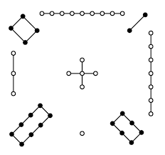
\[=\text{Point}+\text{Lines}+\text{Triangles}+\text{Pyramids}+…\]
Explicit models of such many-body interactions include the \(2\)-body Lennard-Jones potential:
\[V^{(2)}(r)=-V_0\left(2\left(\frac{r_0}{r}\right)^6-\left(\frac{r_0}{r}\right)^{12}\right)\]
the \(3\)-body Stillinger-Weber potential:
\[V^{(3)}(r_1,r_2,\theta)\sim V_0 e^{\sim r_0\left(\frac{1}{r_1-r^*}+\frac{1}{r_2-r^*}\right)}(\cos\theta-\cos\theta_0)^2[r_1<r^*][r_2<r^*]\]
the \(4\)-body potential:
\[V^{(4)}(\mathbf r_1,\mathbf r_2,\mathbf r_3)\sim\left(\frac{\mathbf r_1\cdot(\mathbf r_2\times\mathbf r_3)}{r_1r_2r_3}\right)^2\]
etc.
To compute the \((\nu+1)\)-body interaction term \(\sum_{\langle j_1<…<j_{\nu},i\rangle}\hat V^{(\nu+1)}(\mathbf r_{ij_1},…,\mathbf r_{ij_{\nu}}|Z_i,Z_{j_1},…,Z_{j_{\nu}})\) in ACE (the use of the symbol \(\nu\) as the Greek equivalent of the English letter \(n\) is meant to evoke the concept of “neighbours”), one has to sum \({\nu_i}\choose{\nu}\)\(\in O(\nu_i^{\nu})\) interaction terms which is polynomial in the number \(\nu_i:=|\{\mathbf x_j:r_{ij}<r^*\}|\) of \(r^*\)-neighbours associated to the \(i^{\text{th}}\) atom, but exponential in the number of simultaneous \(r^*\)-neighbours \(\nu\leq\nu_i\).
Fortunately, there exists a simple trick that dramatically simplifies this computation from \(O(\nu_i^{\nu})\to O(\nu_i)\) time. The trick consists of \(2\) steps:
- Step #\(1\): given an arbitrary single-particle basis \(\psi_{\lambda}(\mathbf r)\), expand the \((\nu+1)\)-body potential \(\hat V^{(\nu+1)}(\mathbf r_1,…,\mathbf r_{\nu})\) in that basis:
\[\hat V^{(\nu+1)}(\mathbf r_1,…,\mathbf r_{\nu})=\sum_{\boldsymbol{\lambda}}c_{\boldsymbol{\lambda}}\Psi_{\boldsymbol{\lambda}}(\mathbf r_1,…,\mathbf r_{\nu})\]
where \(\boldsymbol{\lambda}:=(\lambda_1,…,\lambda_{\nu})\) is some \(\nu\)-tuple of valid “eigenvalue quantum numbers” picking out a particular single-particle state \(\psi_{\lambda}\), and \(\Psi_{\boldsymbol{\lambda}}(\mathbf r_1,…,\mathbf r_{\nu}):=\psi_{\lambda_1}(\mathbf r_1)…\psi_{\lambda_{\nu}}(\mathbf r_{\nu})\) is a generic unentangled/separable tensor product of the single-particle “eigenstates” (in practice, one would truncate the space of allowed \(\boldsymbol{\lambda}\)-tuples in the sum \(\sum_{\boldsymbol{\lambda}}\) for approximation purposes).
- Step #\(2\): Interchange the outer sum \(\sum_{\langle j_1<…<j_{\nu},i\rangle}\) with the inner product state \(\psi_{\boldsymbol{\lambda}}(\mathbf r_{ij_1},…,\mathbf r_{ij_{\nu}})\) (a.k.a. a trivial factorization/inversion of the distributive property):
\[\sum_{\langle j_1<…<j_{\nu},i\rangle}\hat V^{(\nu+1)}(\mathbf r_{ij_1},…,\mathbf r_{ij_{\nu}})=\frac{1}{\nu!}\sum_{\boldsymbol{\lambda}}c_{\boldsymbol{\lambda}}A_{i,\boldsymbol{\lambda}}-\text{self-interaction terms}\]
where \(A_{i,\boldsymbol{\lambda}}:=A_{i,\lambda_1}…A_{i,\lambda_{\nu}}\) and \(A_{i,\lambda}:=\sum_{\langle j,i\rangle}\psi_{\lambda}(\mathbf r_{ij})\) (the use of the symbol \(A\) can be justified as a kind of total “amplitude” since it consists of summing the “wavefunction” \(\psi\) at a collection of points).
As currently written, \(SO(3)\) invariance is not guaranteed. The way to remedy this is to convert from the above “\(A\)-basis” to the “\(B\)-basis”, etc. detailed example can be found in the next problem.
Problem: One prominent example of an MLIP is MACE. Walk through a single forward pass of MACE at inference time.
Solution: MACE is an MLIP built on a variant of the MPNN architecture subclass of GNNs. In addition to the standard LAS inductive biases of most MLIPs, MACE itself introduces several further innovations.
The first misconception worth clarifying is that the actual graph input to most MLIPs (including MACE) does not necessarily coincide with how its structural formula might be drawn by a chemist. Instead, the edges are defined solely by the hyperparametric cutoff radius \(r^*\).
With the input undirected graph defined, the rest is just ML (no more physics/chemistry). Just as transformers begin by embedding tokens into latents, here “tokens” can be thought of as vertex features (the atomic numbers \(Z_i\)) and edge features (the translationally-invariant displacement vectors \(\mathbf r_{ij}:=\mathbf x_i-\mathbf x_j\) between vertices). They are learnably and independently embedded as latents:
i) The vertex features \(Z_i\) are embedded by first one-hot encoding \(Z_i\mapsto\hat{\mathbf e}_i\) w.r.t. the size of the periodic table “vocabulary”. These unit one-hots \(\hat{\mathbf e}_i\) are first projected via a linear layer into a latent space of hyperparametric hidden dimension \(d\) (\(d:=128\) is the MACE default), whose \(d\) components indexed by \(k=1,…,d\) shall be denoted \(Z^{(0)}_{i,k00}\). Without any clear motivation yet, it turns out to be fruitful to shift perspective and view this vector as just one step in an initial (\(t=0\)) “double-staircase” feature \(Z^{(0)}_{i,k\ell m}\) initialized with \(Z^{(0)}_{i,k\ell m}:=0\) for all higher angular momentum sectors \(1\leq\ell\leq\ell^*\) (where \(\ell^*\) is another hyperparameter with MACE default \(\ell^*:=3\) capped at \(f\)-wave interactions) and \(-\ell\leq m\leq\ell\).
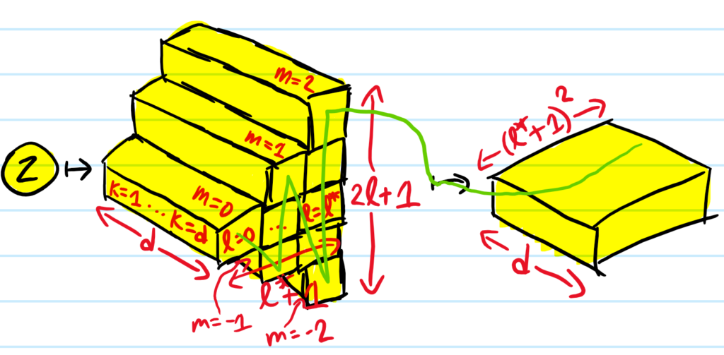
A staircase does not have a well-defined tensor shape, so in practice one concatenates along the \(m\)-axis \(\sum_{\ell=0}^{\ell^*}(2\ell+1)=(\ell^*+1)^2\) to represent the staircase as a PyTorch tensor of shape \((d,(\ell^*+1)^2)\).
ii) The edge features \(\mathbf r_{ij}\) factorize into magnitude and direction features \(\mathbf r_{ij}=r_{ij}\hat{\mathbf r}_{ij}\), which are processed independently before being recombined:
a) The magnitude features \(r_{ij}\) are deterministically embedded as feature vectors \(r_{ij}\mapsto\mathbf R_{ij}:=(R_1(r_{ij}),…,R_{n^*}(r_{ij}))\) (MACE default \(n^*=8\)) where the sinc/\(j_0\) spherical Bessel eigenfunctions of the \(3\)d-Laplacian in the ball \(r<r^*\) are given by \(R_n(r):=\sqrt{\frac{2}{r^*}}\frac{\sin (n\pi r/r^*)}{r}f_p(r)\) (cf. the eigenstates \(\psi_n(x)=\sqrt{\frac{2}{L}}\sin\frac{n\pi x}{L}\) of a quantum particle in the box \(x\in[0,L]\)) modulated by a degree-\((p+2)\) polynomial envelope cutoff \(f_p(r):=\left(1-\frac{(p+1)(p+2)}{2}\left(\frac{r}{r^*}\right)^p+p(p+2)\left(\frac{r}{r^*}\right)^{p+1}-\frac{p(p+1)}{2}\left(\frac{r}{r^*}\right)^{p+2}\right)[r<r^*]\) engineered to obey \(f_p(0)=1\) and \(f_p(r^*)=f’_p(r^*)=f^{\prime\prime}_p(r^*)=0\) (MACE default \(p=5\)). Each of the \(\mathbf R_{ij}\) is then passed through the same MLP (MACE uses \(3\) hidden \(\text{SiLU}\) dense layers in \(64\) dimensions followed by a linear projection output layer). The net effect of this “radial MLP” is thus to map \(\mathbf R_{ij}\in\mathbf R^{n^*}\mapsto\mathbf R’_{ij}\in\mathbf R^{d(\ell^*+1)(\ell^{*2}+2\ell^*+2)/2}\) (using MACE defaults, this is \(d(\ell^*+1)(\ell^{*2}+2\ell^*+2)/2=4352\) output neurons). To understand that output dimension, it helps to realize that although \(\mathbf R’_{ij}\) as depicted is a column vector containing \(d(\ell^*+1)(\ell^{*2}+2\ell^*+2)/2\) elements, it is conceptually better to understand it as possessing the structure \(r_{ij,k\ell_1\ell_2\ell}\) with \(1\leq k\leq d\) (hence the factor of \(d\)) and angular momenta channels \(0\leq\ell_1,\ell_2,\ell\leq\ell^*\) constrained by Clebsch-Gordan selection rules \(|\ell_1-\ell_2|\leq\ell\leq\ell_1+\ell_2\). The number of such triplets \((\ell_1,\ell_2,\ell)\) is given by:
\[\sum_{0\leq\ell_1,\ell_2\leq\ell^*}\left(\text{min}(\ell^*,\ell_1+\ell_2)-|\ell_1-\ell_2|+1\right)\]
\[=\frac{(\ell^*+1)(\ell^{*2}+2\ell^*+2)}{2}\]
which can be easily remembered as it coincides with the magic constant of an \((\ell^*+1)\times (\ell^*+1)\) normal magic square (a coincidence?).
b) The direction features are deterministically encoded as spherical harmonics \(\mathbf Y_{\ell}(\hat{\mathbf r})\in\mathbf C^{2\ell+1}\) with the rotationally equivariant property of transforming under a specific unitary \((2\ell+1)\)-dimensional \(SO(3)\)-irrep \(D^{(\ell)}\) known as the Wigner-\(D\) representation, that is for \(R\in SO(3)\):
\[\mathbf Y_{\ell}(R^{-1}\hat{\mathbf r})=D^{(\ell)}(R)\mathbf Y_{\ell}(\hat{\mathbf r})\]
where \(D^{(\ell)}(R)\in U(2\ell+1)\). Intuitively, a rotation \(\hat{\mathbf r}\mapsto R^{-1}\hat{\mathbf r}\) on \(S^2\) induces a corresponding “rotation” \(\mathbf Y_{\ell}\mapsto D^{(\ell)}(R)\mathbf Y_{\ell}\) in \(\mathbf C^{2\ell+1}\).
Now one gets to the message-passing GNN part:
Message phase: At time step \(t=1,2,..\), the \(j^{\text{th}}\) atom broadcasts a double-staircase message vector \(\boldsymbol{\psi}^{(t)}_{j\to i}\in\mathbf R^{d(\ell^*+1)^2}\) to the \(i^{\text{th}}\) atom whose structured components \(\psi^{(t)}_{j\to i,k\ell m}\) are given by symmetrizing:
\[\psi^{(t)}_{j\to i,k\ell m}:=\sum_{0\leq\ell_1,\ell_2\leq\ell^*}\sum_{|m_1|\leq\ell_1,|m_2|\leq\ell_2}\langle\ell_1,m_1;\ell_2,m_2|\ell m\rangle Z^{(t-1)}_{j,k\ell_1m_1}Y_{\ell_2m_2}(\hat{\mathbf r}_{ij})r_{ij,k\ell_1\ell_2\ell}\]
Aggregation phase: the symbol “\(A\)” stands for “aggregate”:
\[A^{(t)}_{i,k\ell m}:=\sum_{\langle j,i\rangle}\psi^{(t)}_{j\to i,k\ell m}\]
which is simply a pointwise addition of all the double staircase messages.
Update phase: Given \(\boldsymbol{\ell}:=(\ell_1,…,\ell_{\nu})\) and \(\mathbf m:=(m_1,…,m_{\nu})\) Defining \(A^{(t)}_{i,k\boldsymbol{\ell}\mathbf m}:=A^{(t)}_{i,k\ell_1m_1}…A^{(t)}_{i,k\ell_{\nu}m_{\nu}}\), one first has to symmetrize all the double staircase summaries via generalized Clebsch-Gordan coefficients (these are just the obvious generalization to coupling more than \(2\) angular momenta subject to obvious generalized selection rules):
\[B^{(t)}_{i,k\ell m}:=\sum_{\boldsymbol{\ell},\mathbf m}\langle\boldsymbol{\ell},\mathbf m|\ell,m\rangle A^{(t)}_{i,k\boldsymbol{\ell}\mathbf m}\]
Now apply a simple readout layer \(\mathbf R^d\to\mathbf R\) to extract the \(SO(3)\)-invariant local potential at layer \(t\):
\[\hat V_i^{(t)}=\mathbf w^{(t)}\cdot\mathbf B^{(t)}_i\]
where \(\mathbf B^{(t)}_i\) has \(\ell=0\) components \(B^{(t)}_{i,k00}\) for \(k=1,…,d\).
Update the vertex double staircase via a weighted residual skip connection:
\[Z^{(t)}_{i,k\ell m}:=\sum_{k’=1}^d\left(W^{(t)}_{kk’,\ell}Z^{(t-1)}_{i,k’\ell m}+W’^{(t)}_{kk’,\ell}B^{(t)}_{i,k’\ell m}\right)\]
Repeat for \(T\) message passing layers (MACE default \(T:=2\)), and compute the PES as:
\[\hat V(\mathbf x_1,…,\mathbf x_N|Z_1,…,Z_N):=\sum_{i=1}^N\left(E_0(Z_i)+\sum_{t=1}^T\hat V_i^{(t)}\right)\]
Problem: The previous problem describes how MACE operates at inference time. Now explain how MACE is trained.
Solution: In the most general case, the loss function consists of \(3\) MSE terms weighted by relative hyperparameters \(\lambda_V,\lambda_{\mathbf F},\lambda_{\sigma}\):
\[L(\boldsymbol{\theta})=\frac{\lambda_V}{N_{\text{tr}}}\sum_{s=1}^{N_{\text{tr}}}\left(\frac{\hat V(s|\boldsymbol{\theta})-V_s}{N_s}\right)^2\]
\[+\frac{\lambda_{\mathbf F}}{3N_{\text{tot}}}\sum_{s=1}^{N_{\text{tr}}}\sum_{i=1}^{N_s}|\hat{\mathbf F}_i(s|\boldsymbol{\theta})-\mathbf F_{i,s}|^2+\frac{\lambda_{\sigma}}{9N_{\text{tr,per}}}\sum_{s=1}^{N_{\text{tr,per}}}|\hat{\sigma}(s|\boldsymbol{\theta})-\sigma_s|^2\]
where \(s=1,…,N_{\text{tr}}\) can be thought of as indexing each “structure” \(s:=(\mathbf x_1,…,\mathbf x_{N_s},Z_1,…,Z_{N_s})\) containing \(N_s\) atoms in the training dataset, and \(N_{\text{tot}}:=\sum_{s=1}^{N_{\text{tr}}}N_s\) is the total number of atoms in the training dataset.
The stress tensor estimator is computed via \(\hat{\sigma}(s|\boldsymbol{\theta}):=\frac{1}{V_{s,\text{per}}}\sum_{i=1}^{N_s}\mathbf x_i(s)\otimes\hat{\mathbf F}_i(s|\boldsymbol{\theta})=\frac{1}{2V_{s,\text{per}}}\sum_{i=1}^{N_s}\mathbf r_{ij}(s)\otimes\hat{\mathbf F}_i(s|\boldsymbol{\theta})\) and uses the Frobenius norm \(|\sigma|^2:=\text{Tr}(\sigma^T\sigma)\). In practice, any of these MSE losses may also be replaced by a corresponding Huber loss with some hyperparametric \(\delta\)-crossover between the quadratic and linear regimes.
An AdamW optimizer is used with mini-batch SGD, gradient clipping, a learning rate scheduler, etc. the usual. One more thing worth emphasizing is that typically \(\lambda_{\mathbf F}\gg\lambda_V,\lambda_{\sigma}\), the reason being that forces are what actually drive molecular dynamics (MD) simulation and furthermore each training configuration \(s\) with \(N_s\) atoms gives \(3N_s\) loss function signals compared to just a single scalar value for the potential energy.
Problem: Given an MLIP, how does one perform MD simulations with it, and what can one learn from such simulations?
Solution: In the Born-Oppenheimer approximation, the electrons are treated quantum mechanically, the nuclei are treated classically, so the phase space evolution of the nuclei may be numerically evolved according to Newtonian dynamics (possibly with some modifications e.g. if one wants to work in canonical or grand canonical rather than microcanonical ensemble) with the force vector on each nuclei given by the MLIP. The resultant MD may be used to investigate transport phenomena, linear response, phase transitions, mechanical response/defects/fracture, chemical reactions/catalysis, lattice vibrations/anharmonicity, etc. Typical MD simulations may involve \(N_{\text{tot}}\in[10^4,10^6]\) atoms on \(\text{ns}\) to \(\mu\text{s}\) timescales.