Localization of Fast Radio Bursts with a Log-Periodic Dipole Array

As a \(2024\) summer intern in the University of Toronto’s Summer Undergraduate Research Program, I will be working with Dr. Nina Gusinskaia and Dr. Rik van Lieshout (both postdoctoral researchers working jointly at the Canadian Institute for Theoretical Astrophysics (CITA) and the Dunlap Institute for Astronomy & Astrophysics) in the University of Toronto Radio Astronomy and InstrumentatioN Lab (UTRAINLab) headed by Professor Juan Mena-Parra to conduct detailed observational studies of fast radio bursts (FRBs), pulsar scintillometry, and radio interferometry. The purpose of this post is to document my learning journey over the summer with regards to this endeavor. One particularly exciting aspect about this project is that a lot of the pipelines for calibration that I develop can be used eventually for actual projects such as outrigger stations being commissioned in California or BURSTT/KKO projects in Taiwan.

Pulsars

At an astronomy level, a pulsar is just a rotating neutron star (which itself is a misnomer since it’s not really a “star” but actually it’s the corpse of what used to be a fairly massive star! In other words, neutron stars are dead stars). By contrast, at a physics level, a pulsar is a rotating magnetic dipole where in general \(\boldsymbol{\omega}\) and \(\boldsymbol{\mu}\) are not necessarily aligned, giving pulsars their nickname as “cosmic lighthouses”. The magnetic field looks qualitatively like the usual magnetic dipole field \(\textbf B(\textbf x)=\frac{\mu_0}{4\pi}\left(\frac{3(\boldsymbol{\mu}\cdot\hat{\textbf x})\hat{\textbf x}-\boldsymbol{\mu}}{|\textbf x|^3}\right)\). The pulsar’s radius \(R\), density \(\rho\), wavelength \(\lambda\) of emission, and polarization \(\textbf E\) of the light, etc. are all also important parameters to keep in mind.

Pulsars provide a wealth of information about neutron star physics, general relativity, the galactic gravitational potential \(\phi_g(\textbf x,t)\), the galactic magnetic field \(\textbf B_g(\textbf x,t)\), the galactic charge density \(\rho_e(\textbf x,t)\), and more generally many properties (i.e. fields defined on) of the interstellar medium (ISM).

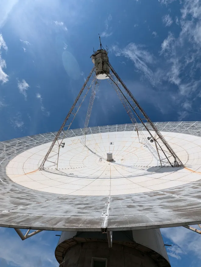
Experimentally, pulsar research is driven by surveys of the cosmos with large radio telescopes (a bit of a misnomer, since it’s not really a “telescope” in the traditional sense of an optical telescope) which are typically parabolic antennas (“dishes”) like the one below designed to focus radio waves:

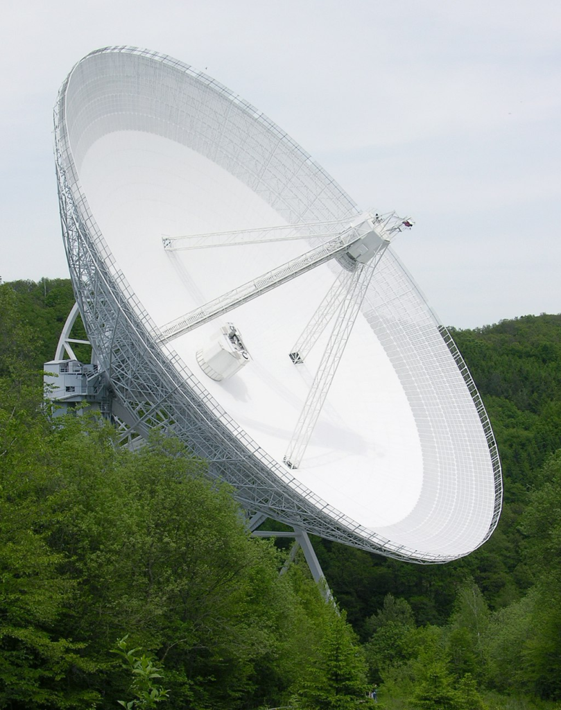
With such large radio telescopes, one challenge is to build them without deformation under their own weight (which would ruin for instance their parabolic surface). A variety of ingenious ways have been devised to solve that problem.

The nomenclature convention for pulsars is to start with “PSR”, followed by “B” or “J” depending on whether it was discovered before or after \(1990\), and then the celestial coordinates of the pulsar.

All binary pulsar systems will eventually coalesce in the limit \(t\to\infty\) due to energy loss via gravitational wave emission.

The pulsar PSR B1937+21 rotates at \(f_{\text{PSR}}=642\text{ Hz}\), which is quite close to the theoretical limit frequency of rotation \(f_{\text{PSR}}^*\).

Pulsars have also been found in globular clusters, with exoplanetary systems, triple systems, and even double pulsars.

Most pulsars to date have been found by the Parkes radio telescope in Australia. Although pulsar astronomy does involve probing across the electromagnetic spectrum, the most important wavelengths are radio.

On a radio telescope antenna, pulsar radio waves are received as “spikes” in the irradiance profile \(I(t)\) received. This irradiance is not in general monochromatic however, but rather is distributed over all frequencies according to \(I=\int_0^{\infty}\rho_I(f)df\) for some spectral irradiance density with respect to frequency \(\rho_I(f)\) measured typically in janskys \(1\text{ Jy}:=10^{-26}\frac{\text W}{\text m^2\cdot\text{Hz}}\). For most pulsars, the spectral irradiance density with respect to frequency is concentrated at low \(f\) (e.g. radio waves). When plotting \(\log(\rho_I(f))\) against \(\log(f)\), one tends to observe a linear decrease in the high-frequency regime \(\log(f)\gg 1\), suggesting a power law dependence of the form \(\rho_I(f)\propto f^{\alpha}\) where \(\alpha<0\) is the spectral index of the pulsar.

In general, if one views the pulsar rotation period \(T_{\text{PSR}}\) as a continuous random variable, then the probability density function \(\rho_{T_{\text{PSR}}}\) of \(T_{\text{PSR}}\) is bimodal, with one hump representing short-period, millisecond pulsars which are more ancient and the other hump representing long-period, younger pulsars with a different evolutionary history. Thus, one seems to find a Heisenberg correlation between time of formation \(\Delta_f t\) and rotation period \(T_{\text{PSR}}\).

Individual pulses from pulsars are very weak radio sources (can only see individual pulses for the “brightest” pulsars). Furthermore, individual pulses turn out to be highly variable due to both stochastic noise and systematic effects (e.g. periodic intensity modulation, drifting sub-pulses, mode changing, nulling, etc.) but if one performs an averaging procedure to obtain a so-called integrated pulse profile \(\bar I(t)\), then, in analogy to the central limit theorem from statistics, one has:

Fundamental “Theorem” of Pulsar Astronomy: the integrated pulse profile \(\bar I(t)\) is stable for \(t\in\textbf R\).

Since pulsars tend to be very polarized, a well-calibrated polarimeter can offer accurate determination of \(4\) Stokes parameters \(S_0,S_1,S_2,S_3\) which can be combined into a Stokes vector \(\textbf S:=(S_0,S_1,S_2,S_3)^T\in\textbf R^4\). The precise definitions of each the \(S_i\) is in terms of certain electric field components, though in essence the Stokes vector provides a bijection with all possible elliptic polarization of light from the pulsar. As this polarized light propagates through the ISM, it also undergoes Faraday rotation due to the galactic magnetic field \(\textbf B_g\) with the spatial rate \(\frac{\partial\theta}{\partial x}\) of such Faraday rotation being proportional to \(\textbf B_g\cdot\textbf k\) where \(\textbf k\) is the angular wavevector and the constant of proportionality is called the Verdet constant.

By applying a simple harmonic oscillator model to the ISM as an electron plasma, one can show that the time \(\Delta t\) required for light of frequency \(f\) to reach Earth from a pulsar a distance \(d\) away is:

\[\Delta t=\frac{d}{c}+\frac{e^2}{2\pi m_{e^-}cf^2}\int_0^dn_{e^-}d\ell\]

where the line integral \(\int_0^dn_{e^-}d\ell\) is taken along the line of sight between the pulsar and Earth and is called the dispersion measure of the pulsar since it determines the degree to which the interstellar medium optically disperses the various frequencies of light from the pulsar (units of the dispersion measure are typically \(\text{pc}/\text{cm}^3\)). This can be used to map out the \(e^-\) density of the galaxy.

Contrary to what one might intuitively expect, the interstellar medium is actually a turbulent and non-uniform fluid (more precisely an electron plasma). This is directly responsible for a sort of interstellar scintillation effect (analogous to how turbulence in the atmosphere causes star light to twinkle, except here the scintillation/twinkling effect is for radio waves rather than visible light). Quantitatively, one can adapt a very simple thin screen model to model the interstellar medium, one prediction of which is that interstellar scintillation broadens the frequency spectrum by some scintillation bandwidth \(\Delta f\) which is proportional to \(f^4\) (where \(f\) is the observing frequency). This manifests as an exponential tail in plots of \(I(t)\) for folded pulsar signals, where the time scale \(\tau_s\propto\frac{1}{\Delta f}\propto\frac{1}{f^4}\) of such an exponential decay is called the scattering time and in the thin-screen model is explained by variations in mean free path. Obviously, a larger \(\tau_s\) is undesirable because it implies a broader pulse, hence a lower SNR. This means that radio telescopes generally should observe at higher \(f\) (e.g. the Parkes radio telescope’s multibeam galactic plane survey at \(f=1.4\text{ GHz}\) discovered much more dispersed and scattered pulsars than previous low-\(f\) surveys (although actually observing is never at a single frequency \(f\), but rather in some bandwidth of frequencies \([f-\Delta f/2,f+\Delta f/2]\).

Finally, a bit about the population statistics of pulsars. Most, by observational bias, have been found in the Milky Way’s galactic plane and in particular near our Solar System. As pulsars emit radiation (rotating magnetic dipoles!), they lose rotational kinetic energy. As this energy drops, therefore their rotational period \(T\) increases \(\dot T>0\). In general, both \(T\) and \(\dot T\) can be obtained precisely via timing measurements. Therefore, if one plots \(\log(T)\) vs. \(\log(\dot T)\), one finds a clear separation of pulsars into “normal” pulsars in the upper right quadrant and millisecond pulsars in the bottom left.

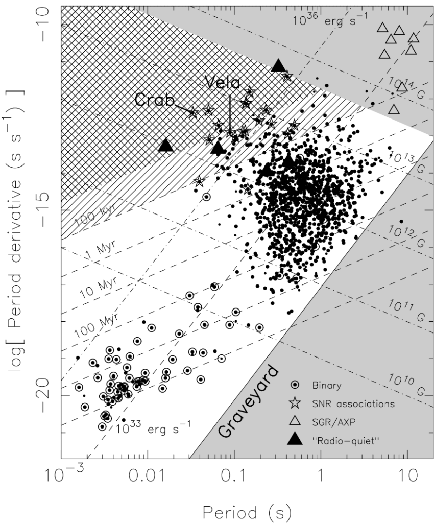
It can be shown from a simple rotating magnetic dipole model that:

\[t_{\text{age}}\propto\frac{T}{\dot T}\]

\[B\propto\sqrt{T\dot T}\]

\[\dot E\propto\frac{\dot T}{T^3}\]

Quite naturally, this data suggests that pulsars begin as “normal” pulsars and then at some point rapidly spin down into the millisecond pulsars domain (the rapid nature of this spin down process would explain why there are no pulsars intermediate). It is also interesting to note that most binary pulsars (not necessarily \(2\) pulsars orbiting each other but just a pulsar orbiting another celestial object) are in the millisecond pulsars category).

Antenna Fundamentals

Roughly speaking, in the lingo of particle physics, an antenna is any conductor that mediates interactions between photons \(\gamma\) and electrons \(e^-\). That is:

\[\gamma\leftrightarrow e^-\]

More precisely, thinking of photons \(\gamma\) in the classical way as propagating electromagnetic \((\textbf E,\textbf B)\) waves, an antenna can be used either as a transmitting antenna meaning that an external driving voltage source \(V\) (called a transmitter and which needs to be impedance-matched \(Z_{\text{transmitter}}=Z_{\text{antenna}}^{\dagger}\) with the antenna via an antenna tuner circuit to maximize power delivery to the antenna rather than allow the power to “reflect” from the antenna back to the transmitter and form standing waves) induces a corresponding AC current \(I=V/Z_{\text{antenna}}\) in the antenna so that accelerating electrons \(e^-\) will emit electromagnetic radiation (photons \(\gamma\)); thus for a transmitting antenna one has \(e^-\to\gamma\). By contrast, the same antenna can also be used as a receiving antenna so external electromagnetic waves (e.g. from celestial sources, terrestrial interference, etc.) exert a Lorentz force \(\textbf f=\rho\textbf E+\textbf J\times\textbf B\) on the electrons \(e^-\) in the antenna, causing them to slosh into an AC current \(I\) (which is then recorded by an impedance-matched receiver unit); thus for a receiving antenna \(\gamma\to e^-\).

As one might expect, transmitting antennas might transmit EM radiation better in some directions \(\hat{\textbf n}\) than others, and similarly receiving antennas may be more sensitive to EM radiation coming from some directions \(\hat{\textbf n}\) than others. This is quantified by the directivity of the antenna \(D:S^2\to[0,\infty)\) which maps each direction \(\hat{\textbf n}\in S^2\) on the celestial sphere \(S^2\) to a dimensionless non-negative real number \(D(\hat{\textbf n})\geq 0\) describing how “directed” the antenna is in that direction \(\hat{\textbf n}\):

\[D(\hat{\textbf n}):=\frac{\hat P(\hat{\textbf n})}{\overline{\hat P}}\]

where \(\hat P\) is the power per unit solid angle (SI units: \(\text W/\text{sr}\)) on \(S^2\) so that the total power of the entire sky would be given by \(P=\iint_{\hat{\textbf n}\in S^2}\hat P(\hat{\textbf n})d^2\hat{\textbf n}\) and \(\overline{\hat P}=P/4\pi\) is the average power per unit solid angle.

The maximum directivity \(D^*\in [1,\infty)\) (also just called the directivity if no direction \(\hat{\textbf n}\) is specified) is simply:

\[D^*:=\sup_{\hat{\textbf n}\in S^2}D(\hat{\textbf n})\]

and is usually expressed in decibels \(D^*_{\text{dBi}}=10\log(D^*)\). For instance, an (idealized, theoretical, not-actually-a-thing) isotropic antenna by definition exhibits an isotropic power profile \(\hat P(\hat{\textbf n})=P_0\) for some constant \(P_0\) across the sky \(S^2\) so that it also exhibits an isotropic directivity \(D(\hat{\textbf n})=1\) and correspondingly \(D^*=1\) or \(D^*_{\text{dB}}=0\text{ dBi}\) (the minimum possible maximum directivity!). This explains why the logarithmic form \(D^*\) has decibel units called “dBi” since the “i” stands for “isotropic”, implying that the decibel comparison is with the isotropic antenna \(D^*_{\text{dBi}}=10\log(D^*)=10\log(D^*/1)\).

One might worry that there should be a need to distinguish between \(D_{\text{transmitting}}\) and \(D_{\text{receiving}}\), i.e. that the antenna may have different directivities depending on whether it’s being used as a transmitting antenna or a receiving antenna. Fortunately, a deep symmetry of Maxwell’s equations known as electromagnetic reciprocity guarantees, among other corollaries, that the transmitting and receiving directivities for any antenna are identical, i.e.

\[D_{\text{transmitting}}(\hat{\textbf n})=D_{\text{receiving}}(\hat{\textbf n}):=D(\hat{\textbf n})\]

(more precisely, electromagnetic reciprocity holds for passive antennas, not for active antennas). However, in practice the directivity isn’t the only factor that one cares about; there is also the transmission line (often coaxial cable for radio applications) between the antennas and transmitter/receiver units so that one is not just interested in the directivity \(D(\hat{\textbf n})\) of the antenna but also its gain \(G(\hat{\textbf n})\in [0,\infty)\), which is proportional to its directivity \(G(\hat{\textbf n}):=\eta D(\hat{\textbf n})\) where the constant of proportionality \(\eta\in[0,1]\) is called the radiation efficiency and is defined in the obvious manner by the ratio:

\[\eta:=\frac{P_{\text{output}}}{P_{\text{input}}}\]

More precisely, for a transmitting antenna, \(\eta=P_{\text{antenna}\to S^2}/P_{\text{transmitter}\to\text{antenna}}\) whereas for a receiving antenna, \(\eta=P_{\text{antenna}\to\text{receiver}}/P_{S^2\to\text{antenna}}\). Combining with the previous definition of directivity (where the notation \(P\) was used for what is being denoted by \(P_{\text{output}}\) above), one can also write \(G(\hat{\textbf n})=4\pi\hat{P}(\hat{\textbf n})/P_{\text{input}}\). Finally, it is also common to speak of the maximum gain \(G^*:=\eta D^*\) (or just gain if no direction is given) and as with directivities, it is conventional to express gains logarithmically \(G_{dBi}:=10\log(G)\).

One common way of studying an antenna is to plot its gain profile \(G(\hat{\textbf n})\) (or some planar cross-section thereof) in polar coordinates. For instance,

Radio Interferometry

There are several benefits enjoyed by radio astronomy which are not enjoyed by optical astronomy.

To start, it suffices to consider the case of cross-correlating just \(N=2\) radio telescopes, since a more general array of \(N\) radio telescopes is equivalent to \(\frac{N(N-1)}{2}\) pairs of radio telescopes, thus growing quadratically in \(N\) (e.g. the Atacama Large Millimeter/Submillimeter Array (ALMA) in Chile boasts \(N=66\) radio telescopes, yielding a total of \(2145\) pairs of radio telescopes).

The (complex) visibility \(V(u,v)\) is defined to be … it is then a non-trivial result of optical coherence theory known as the van Cittert-Zernike theorem (intuitively, the geometric effect that a sum of incoherent waves will become more spatially coherent with propagation distance). that the complex visibility is also the Fourier transform of the spectral radiance of the sky (thus, the correlator (multiply, time-avg) approach of the electronics is supposed to agree with this Fourier transform). There are two kinds of optical coherence: spatial coherence and temporal coherence. Thus, the fundamental theorem of radio interferometry is:

\[C_{jk}(f, t)=\iint_{\hat{\textbf n}\in S^2}\tilde{\rho}_I(\hat{\textbf n})e^{-ik(\Delta\textbf x\cdot\hat{\textbf n})}d\Omega\]

valid in the “flat-sky limit” on the tangent space \(T_{\hat{\textbf n}}(S^2)\) on the celestial sphere. Apparently there may also be some gain term in front of the spectral irradiance term \(\tilde{\rho}_I=\tilde{\rho}_I(\hat{\textbf n},\omega)\) (SI units: W/(m^2*Hz*sr)). Intuitive interpretation is to write \(\tilde{\rho}_I(\hat{\textbf n})d\Omega=d{\rho}_I(\hat{\textbf n})\), so think of a continuous phasor addition which is what the integral is trying to accomplish.

Apparently the 2D case of a Fourier transform is a special case resulting from a more general non-Fourier 3D case…and what does it all have to do with commuting with translations?

Given an array of \(N\) radio telescopes at positions \(\textbf x_1,\textbf x_2,…,\textbf x_N\), the maximum separation \(\text{max}_{1\leq i,j\leq N}|\textbf x_i-\textbf x_j|\) determines the minimum angular resolution of the array whereas the minimum separation \(\text{min}_{1\leq i,j\leq N}|\textbf x_i-\textbf x_j|\) determines the maximum angular size.

The key method of interferometry is called aperture synthesis…Earth-rotation aperture synthesis as viewed from an object.

The idea behind beamforming is that

If a fixed voltage \(V\) is connected across two resistors \(R_1,R_2\) in series, and one resistor \(R_1\) is fixed, then what value of resistance \(R_2\) should one select to maximize the power dissipated \(P_2\) in \(R_2\)? The answer (found from a simple calculation) is \(R_2=R_1\), i.e. the resistances need to match. More generally, for two loads with arbitrary impedances \(Z_1,Z_2\) in series, the idea is that real power is only dissipated by any resistive components \(\text{Re}(Z_1),\text{Re}(Z_2)\) in the circuit. Thus, if one wishes to maximize the real power dissipated by \(Z_2\) (with \(Z_1\) fixed as in the first case), then one should align the real components as much as possible while getting the imaginary components to cancel out. This leads to the impedance-matching criterion: \(Z_2=Z_1^{\dagger}\). For a radio reflector telescope, the antenna \(Z_1\) is typically impedance-matched with a resistive load \(R_2\)?

A transmitting antenna maps AC voltages/currents in a conductor to electromagnetic waves whereas a receiving antenna is the inverse map. A corollary of electromagnetic reciprocity is that if an antenna \(\mathcal A\) is used as a transmitting antenna, then its transmission pattern will be identical to its reception pattern if \(\matchal A\) were to instead be used as a receiving antenna.

A simple model of an antenna is known as a Hertzian dipole and consists of an infinitesimal wire of length \(dx\) passing an AC current \(I(t)=I_0e^{i\omega_{\text{ext}}t}\). Then the corresponding infinitesimal electric and magnetic fields can be shown (many possible ways) to be:

\[d\textbf E=\sqrt{\frac{\mu_0}{\varepsilon_0}}\frac{Idx}{4\pi}e^{-ikr}[2\left(\frac{1}{r^2}-\frac{i}{kr^3}\right)\textbf r_{\theta,\phi}+\left(\frac{ik}{r}+\frac{1}{r^2}-\frac{i}{kr^3}\right)\sin(\theta)\boldsymbol{\theta}_{\theta,\phi}]\]

\[d\textbf B=\]

Recall that the Jones vector \(\hat{\textbf E}_0\) of a planar electromagnetic wave travelling in the \(z\)-direction is defined to satisfy \(\textbf E(z,t)=\Re(E_0\hat{\textbf E}_0e^{i(kz-\omega t)})\) and note that quantum mechanically the Jones vector \(\hat{\textbf E}_0\in\textbf C^2\) is the same as the polarization state \(|\psi\rangle\in\textbf C^2\) of the photon associated to that EM wave. The coherency/correlation/visibility operator \(C\) is then defined as a projection operator \(C^2=C\) that maps \(\textbf C^2\) onto the span of the Jones vector \(\hat{\textbf E}_0\in\textbf C^2\), and is commonly represented in the same orthonormal basis of \(\textbf C^2\) that the Jones vector is represented in.

\[C:=\hat{\textbf E_0}\hat{\textbf E_0}^{\dagger}=|\hat{\textbf E_0}\rangle\langle\hat{\textbf E_0}|=\hat{\textbf E_0}\otimes\hat{\textbf E_0}\]

or, in any orthonormal basis \(\beta\) of \(\textbf C^2\), one has the explicit matrix representation

\[[C]_{\beta}^{\beta}=\frac{1}{2}(S_0\sigma_0+S_2\sigma_1-S_3\sigma_2+S_1\sigma_3)\]

where \(\textbf S:=(S_0,S_1,S_2,S_3)^T\) is the Stokes vector consisting of \(4\) Stokes parameters and \(\sigma_0,\sigma_1,\sigma_2,\sigma_3\) are the Pauli matrices in the physicist’s convention. Thus, the \(2\times 2\) matrix \(S_0\sigma_0+S_2\sigma_1-S_3\sigma_2+S_1\sigma_3\) represents a general Hermitian matrix in \(i\frak u\)\((2)\).

Noise

Johnson-Nyquist noise (also called thermal noise) is a fundamental, unavoidable source of noise in any electronics. Its origin lies in the thermal agitation of electrons in any conductor, even one that would normally be considered to be in “electrostatic” equilibrium. For radio receivers (also called radiometers in astronomy) Johnson-Nyquist noise can drown out weak radio signals received by a radio telescope. The root-mean-square voltage fluctuations \(\Delta V_{\text{RMS}}^{\text{JN}}=2\sqrt{kTR\Delta f}\) clearly increases with temperature \(T\) as expected, and so radio receivers often need to be cooled to cryogenic temperatures to minimize Johnson-Nyquist noise.

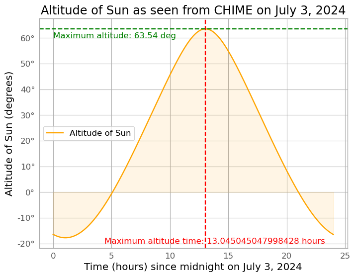
In the project, a log-periodic dipole (antenna) array (LPDA) has been built in Algonquin National Park’s Radio Observatory (ARO). The LPDA is inclined at an angle \(\theta\) such that it “observes” (or more precisely, receives radio waves from) the same patch of sky that the Canadian Hydrogen Intensity Mapping Experiment (CHIME) radio telescope array in British Columbia, Canada, also observes. At \(\lambda_{\text{CHIME}}=-119.6629^{\circ}\) and \(\phi_{\text{CHIME}}=49.3206^{\circ}\). Pip installing the free and open source AstroPy library in Microsoft VS Code’s terminal, I was then able to create a plot of the Sun’s altitude \(h(t)\) above the horizon as a function of time \(t\) since midnight (i.e. the start of the day) for July \(3\)rd, \(2024\):

One of the key objectives of this project is to investigate, using the LPDA antenna in ARO, the mysterious giant pulses that are occasionally emitted by the Crab pulsar (the pulsar left over from the Crab Nebula \(\text M1\) which is a misnomer because it’s not actually a nebula but a supernova remanent). To do so, one must first perform a meticulous complex gain calibration of the antenna.

Complex Gain Self-Calibration

Each antenna \(j=1,2,…,8\) of the LPDA array receives radio waves from various celestial and terrestrial sources, giving rise to a voltage \(V_j(f,t)=\).

Thus, after the normalization change of variables, the problem reduces to minimizing the following standard \(\chi^2:\textbf C^8\to [0,\infty)\) cost function for the visibility matrix:

\[\chi^2(\textbf g):=\text{Tr}(C(f,t)-\textbf g\textbf g^{\dagger})^{\dagger}(C-\textbf g\textbf g^{\dagger})\]

this can be viewed as a form of maximum likelihood estimation (MLE) (does it come from log-likelihood of product of uncorrelated Gaussians?). In other words, one would like to minimize the Frobenius norm squared of \(C-\textbf g\textbf g^{\dagger}\). First, notice that actually \((C-\textbf g\textbf g^{\dagger})^{\dagger}=C-\textbf g\textbf g^{\dagger}\) is Hermitian, so one has:

\[\chi^2=\text{Tr}(C(f,t)-\textbf g(f,t)\textbf g(f,t)^{\dagger})^2\]

Expanding this out and using linearity of \(\text{Tr}\) gives:

\[\frac{\partial\chi^2}{\partial\textbf g}=\frac{\partial}{\partial\textbf g}\text{Tr}(C^2)-\frac{\partial}{\partial\textbf g}\text{Tr}(C\textbf g\textbf g^{\dagger})-\frac{\partial}{\partial\textbf g}\text{Tr}(\textbf g\textbf g^{\dagger}C)+\frac{\partial}{\partial\textbf g}\text{Tr}(\textbf g\textbf g^{\dagger}\textbf g\textbf g^{\dagger})\]

Recall that \(\text{Tr}(AB)=\text{Tr}(BA)\) and \(\textbf g^{\dagger}\textbf g=|\textbf g|^2=\text{Tr}(\textbf g\textbf g^{\dagger}\) (i.e. the Frobenius norm of a vector agrees with its usual Euclidean norm), so:

\[\frac{\partial\chi^2}{\partial\textbf g}=-2\frac{\partial}{\partial\textbf g}\text{Tr}(C\textbf g\textbf g^{\dagger})+\frac{\partial}{\partial\textbf g}|\textbf g|^4\]

Then, using the complex matrix calculus identities \(\frac{\partial\text{Tr(AXB)}}{\partial X}=(BA)^{\dagger}\) and \(\frac{\partial\text{Tr(AX^TB)}}{\partial X}=BA\) with the product rule, it follows that the complex gradient of the \(\chi^2\) cost function is:

\[\frac{\partial\chi^2}{\partial\textbf g}=-2\left((\textbf g^{\dagger}C)^{\dagger}+C\textbf g\right)+4|\textbf g|^2\textbf g=4(|\textbf g|^2\textbf g-C\textbf g)\]

From this, it thus follows that stationary points \(\frac{\partial\chi^2}{\partial\textbf g}=\textbf 0\) occur precisely when \(C\textbf g=|\textbf g|^2\textbf g\), so the complex gain vector \(\textbf g\) is an eigenvector of the visibility matrix \(C\) with eigenvalue \(|\textbf g|^2\). However, not all of these eigenvectors are minima of \(\chi^2\). To analyze this stability, one can first look at the Jacobian \(\frac{\partial^2\chi^2}{\partial\textbf g^2}\) of \(\frac{\partial\chi^2}{\partial\textbf g}\) (i.e. the Hessian of \(\chi^2\)):

\[\frac{\partial^2\chi^2}{\partial\textbf g^2}=4\frac{\partial}{\partial\textbf g}(|\textbf g|^2\textbf g-C\textbf g)=4(2\textbf g\textbf g^{\dagger}+|\textbf g|^21-C)\]

To do so, it turns out to be convenient to use the Sun, the radio source Cygnus A (Cyg A) and the radio source Cassiopeia A (Cas A). RAM ring buffer 2 minute circle, transit times of 1 hour or so for Sun, don’t need a lot of accuracy, one first must pscreen in linux system dscript. Bash script, curl command, Unix time… After a lot of polishing, this Python script was finally polished into:

# Import the necessary Python libraries for calculating meridian transits, interfacing
# with the local operating system that this Python script is run on (in this case, will
# be the cloyd Unix machine at ARO) and for time keeping
import numpy as np
import os
import time
import datetime
import dateutil.parser as dp
import astropy.units as u
from astropy.coordinates import AltAz, EarthLocation, get_sun, SkyCoord
from astropy.time import Time
import pytz

# Location of observation (technically observing from ARO, but antennas are pointed at CHIME zenith)
CHIME_latitude = 49.3206 #degrees
CHIME_longitude = -119.6229 #degrees
CHIME_height = 500 #meters
CHIME_location = EarthLocation(lat = CHIME_latitude * u.deg,
                               lon = CHIME_longitude * u.deg, 
                               height = CHIME_height * u.m)

# Number of time steps over which to calculate altitude h(t) and hence compute next transit times
# of celestial objects in the compute_next_transit_time function defined below
number_of_time_steps = 10000
time_steps = np.linspace(0, 23.935, number_of_time_steps) * u.hour # sidereal day, not solar day

def compute_next_transit_time(celestial_object):
    """
    When this Python script is run, the function compute_next_transit_time returns the next time
    that an arbitrary celestial object (the only input into the function) will 
    pass over the local meridian of the CHIME telescope in Vancouver, British Columbia, Canada
    relative to the time that the script was run. The function works by calculating
    the altitude h(t) of the celestial object as a function of time t for a duration of 24 hours
    starting from the time that the script was run. More precisely, these 24 hours are chopped into 
    an arbitrary number of time steps (a global variable in this script) and the altitude h(t) of 
    the celestial object is calculated at each time step. The function then finds the time t when
    h(t) is maximized and returns this time as the next transit time of the celestial object. 
    Increasing the number of time steps will result in a more accurate calculation of the
    next transit time of the celestial object at the cost of increased computational time.

    Parameters
    ----------
    celestial_object : SkyCoord object (required)
        The celestial object of interest (e.g. the Sun, Cygnus A, Cas A, etc.) that is being
        observed by the CHIME telescope.
    
    Returns
    -------
    Next transit time of the celestial object as an astropy Time object
    """
    times_array = Time(datetime.datetime.now(pytz.timezone("UTC"))) + time_steps 
    frames = AltAz(obstime=times_array, location=CHIME_location)
    alt_az_data = celestial_object.transform_to(frames)
    return alt_az_data.obstime[np.argmax(alt_az_data.alt)]

# Time window that transit should be considered for (e.g. 900 seconds means total transit time
# window is 1800 seconds or 30 minutes)
transit_time_window_plus_minus = 900 #seconds

# Time after the hour that the weather station is transmitting radio waves for (e.g. 300 seconds 
# means the weather station is transmitting radio waves for 300 seconds after the hour).
weather_station_time_window = 300 

command_prefix = "curl -H \'Content-Type: application/json\' -d \'{" 
def kotekan_trigger_command(celestial_object_id):
    """
    This function defines the syntax of the command that needs to be executed on a local 
    Unix-like operating system to trigger the Kotekan script to dump baseband data from 
    the RAM ring buffer to the SSD on cloyd. The command is a curl command that sends 
    a JSON object to the Kotekan server running on cloyd. The JSON object contains the 
    event ID of the celestial object that is currently in transit, the file path where 
    the baseband data should be dumped, the start time of the baseband dump, the 
    duration of the baseband dump, and the dispersion measure (dm) of the celestial object.
    Note that as with the compute_next_transit_time function, this function stores a live
    time stamp of when the command is executed and uses this time stamp to generate a unique
    event ID for the celestial object that is currently in transit.
    """
    current_UTC_time = datetime.datetime.now(pytz.timezone("UTC"))
    event_id = "1" + str(celestial_object_id) + current_UTC_time.strftime("%Y%m%d%H%M%S")
    start_unix_seconds = current_UTC_time.timestamp() - 10
    return command_prefix + ("\'event_id\': %d" %int(event_id) 
                          + ",\'file_path\': \'dummy\'" 
                          + ", \'start_unix_seconds\': %d}" %int(start_unix_seconds) 
                          + ", \'start_unix_nano\': 0, \'duration_nano\': 100000000" 
                          + ", \'dm\': 0.0, \"dm_error\": 0}\'"
                          + "localhost:12048/baseband")

def baseband_data_dump_protocol(celestial_object_id):
    """
    This function defines the protocol for dumping raw baseband data from the RAM ring buffer
    into the SSD on cloyd. It is triggered whenever any celestial object is in transit. 
    It performs a baseband dump once every 1/3 of a transit time window and sleeps in 
    between. This continues happening until the object is no longer in transit.
    """
    UTC_time_now = dp.parse(str(datetime.datetime.now(pytz.timezone("UTC")))[:26]).timestamp()
    next_transit_time = celestial_objects_next_transit_times[celestial_object_id]
    transit_time = dp.parse(str(next_transit_time.value)).timestamp()
    number_of_baseband_dumps = 3

    while np.abs(transit_time - UTC_time_now) < transit_time_window_plus_minus:
        print("Celestial object with ID: " 
             + str(celestial_object_id) 
             + " is in transit!"
             + " Triggering Kotekan in cloyd to dump baseband data"
             + " from RAM ring buffer into the SSD!")
        os.system(kotekan_trigger_command(celestial_object_id))
        print(kotekan_trigger_command(celestial_object_id))
        time.sleep(2*transit_time_window_plus_minus/number_of_baseband_dumps)

    print(str(celestial_object_id) 
        + " has finished transitting the meridian of CHIME!"
        + " Updating next transit time.")
    next_transit_time = compute_next_transit_time(celestial_object)

# Daemonize this Python script on the cloyd Unix machine using the while loop. First, check if the
# weather station is transmitting radio waves. If it is, sleep for the duration of the time window
# that the weather station is transmitting radio waves. If the weather station is not transmitting
# radio waves, check if any celestial objects are in transit. If they are, trigger the Kotekan script
# to dump baseband data from the RAM ring buffer to the SSD on cloyd. Sleep for 1/3 of the total
# transit time window and repeat the process until the celestial object is no longer in transit.
# If no celestial objects are in transit, sleep until the next transit time window of the next
# celestial object in the list of celestial objects of interest.
while True:
    # Store the current UTC time
    UTC_time_now = dp.parse(str(datetime.datetime.now(pytz.timezone("UTC")))[:26]).timestamp()
    UTC_hour_now = dp.parse(str(datetime.datetime.now(pytz.timezone("UTC")))[:14] + "00:00").timestamp()

    # Defining celestial objects of interest (all 3 are bright radio sources). Sun is for 
    # gain calibration of the LPDA array while Cyg A and Cas A are for testing its sensitivity.
    Sun = get_sun(Time(datetime.datetime.now(pytz.timezone("UTC"))) 
                + time_steps)
    Cyg_A = SkyCoord.from_name("Cyg A") 
    Cas_A = SkyCoord.from_name("Cas A") 

    # New celestial objects need to be added manually to these lists
    celestial_objects = [Sun, 
                         Cyg_A, 
                         Cas_A] 
    celestial_object_names = ["Sun", 
                              "Cygnus A", 
                              "Cassiopeia A"]
    
    # Next meridian transit times for celestial objects of interest at CHIME
    celestial_objects_next_transit_times = []
    for celestial_object in celestial_objects:
        celestial_objects_next_transit_times.append(compute_next_transit_time(celestial_object))

    print("Current UTC time is: "
         + str(datetime.datetime.now(pytz.timezone("UTC")))) 
    print("Celestial Objects Next Transit Times: " 
         + str(list(zip(celestial_object_names, celestial_objects_next_transit_times))))

    if (UTC_time_now - UTC_hour_now < weather_station_time_window):
        print("Weather station is transmitting radio waves! Sleeping for: " 
             + str(weather_station_time_window) 
             + " seconds.")
        time.sleep(weather_station_time_window)
    else:
        for celestial_object_id in np.arange(0, len(celestial_objects), 1):
            next_transit_time_object = celestial_objects_next_transit_times[celestial_object_id]
            next_transit_time_value = dp.parse(str(next_transit_time_object.value)).timestamp()
            if np.abs(next_transit_time_value - UTC_time_now) < transit_time_window_plus_minus:
                baseband_data_dump_protocol(celestial_object_id)
            else: 
                print("Celestial object " 
                     + str(celestial_object_names[celestial_object_id])
                     + " with celestial object ID "
                     + str(celestial_object_id)
                     + " is not in transit at the moment.")
    next_transitting_celestial_object_id = np.argmin([t.value for t in celestial_objects_next_transit_times])
    next_transit_time_object = celestial_objects_next_transit_times[next_transitting_celestial_object_id]
    next_transit_time_value = dp.parse(str(next_transit_time_object.value)).timestamp()
    print("Next transitting celestial object is " 
         + str(celestial_object_names[next_transitting_celestial_object_id])
         + " with celestial object ID "
         + str(next_transitting_celestial_object_id))
    time_until_next_transit_time_window = next_transit_time_value - UTC_time_now - transit_time_window_plus_minus
    print("Sleeping for: " 
         + str(time_until_next_transit_time_window//3600) 
         + " hours, "
         + str((time_until_next_transit_time_window%3600)//60)
         + " minutes, and "
         + str(time_until_next_transit_time_window%60)
         + " seconds until that celestial object will transit!")
    time.sleep(time_until_next_transit_time_window)

The simplest form a radio interferometer is two radio telescopes both receiving radio waves from a distant source in direction \(\hat{\textbf n}\) on the celestial sphere (Fraunhofer, assume plane waves). If \(\Delta\textbf x\) denotes the baseline vector between the two radio telescopes, then there exists a geometric delay \(\Delta t_g=\Delta\textbf x\cdot\hat{\textbf n}/c\) between the two radio telescope antenna AC voltage signals in the sense that if one antenna receives an AC voltage of the form \(V_1(t)=V_0\cos(\omega t)\) where \(V_0\) is the amplitude and \(\omega\) is the angular frequency of the radio waves being received, then the second radio telescope antenna will receive an AC voltage of the form \(V_2(t)=V_0\cos(\omega(t-\Delta t_g))\) delayed in time by the geometric delay \(\Delta t_g\). These two AC voltages may be amplified by some electronics, and then passed into a piece of electronics which effectively acts as a correlator \((V_1(t),V_2(t))\mapsto \langle V_1V_2\rangle\in\textbf R\) which in this case yields a time-averaged product of voltages \(\langle V_1V_2\rangle=\frac{1}{2}V_0^2\cos(\omega\Delta t_g)\). This has the effect of filtering out high frequencies (low-pass filter).

To experimentally measure the geometric delay \(\Delta t_g\) between a pair of radio telescopes, the fundamental insight is that the cross-correlation \(V_1\star V_2(\Delta t)\) is maximized when \(\Delta t=\Delta t_g\), i.e. \((\frac{d(V_1\star V_2)}{d\Delta t})_{\Delta t=\Delta t_g}=0\). Strictly speaking, this only gives the total delay between a pair of antennas which will mostly be made up of geometric delay \(\Delta t_g\) but as I found out in this project, may also experience a contribution from cable delay \(\Delta t_c\) due to slightly different cable lengths (that’s how sensitive interferometry needs to be).

Another effect is aliasing (Shannon-Nyquist theorem?). This arises due to periodicity \(\cos(\phi+2\pi n)=\cos(\phi)\) for all \(n\in\textbf Z\), so if the path length difference is some multiple of wavelength of radio waves, then one might as well think that the radio waves at both radio telescopes are in phase and think that the object is directly overhead in the zenith when clearly that may not be the case. Not to be confused with the notion of an alias in computer programming.

One useful plot to consider is a \(2\)-D color plot of phase \(\phi(t,f)\) in the time-frequency domain \((t,f)\in\textbf R^2\). Specifically, the idea is that radio waves from celestial sources will typically not be monochromatic (i.e. containing only one frequency \(f\)) but rather will have a spectral irradiance density \(\rho_I(f)\) which is distributed in \(f\)-space. For a source in a given direction \(\hat{\textbf n}\), these different Fourier components are emitted in-phase from the celestial source, but for two radio telescopes separated by baseline \(\Delta\textbf x\), the phase discrepancy seen by the two radio telescopes will be \(\Delta\phi=\frac{2\pi f\Delta\textbf x\cdot\hat{\textbf n}}{c}\) a linear function of the frequency \(f\). However, the path length difference \(\Delta\textbf x\cdot\hat{\textbf n}\) is a function of time \(t\) because of the Earth’s rotation. This means that the overall phase \(\Delta\phi\) depends on both \(t\) and \(f\) and so a suitable \(2\pi\)-periodic coloring scheme can be used to illustrate this.

Linux

As part of this project, I had to learn a bit about how to use the Linux operating system (known less commonly as GNU/Linux as Linux was strictly speaking only the kernel of what we now call Linux). It is not to be confused with the Unix operating system, though both use very similar programming syntax (indeed, Linux came after and was based on Unix, so one often says that Linux is a Unix clone or a Unix-like operating system). One key difference between the two operating systems is that Linux is free and open-source whereas Unix requires a paid license to use (i.e. it is proprietary software, just like Microsoft Windows). In order to actually use Linux on a personal computer (PC), one requires the installation of a Linux distribution (distro). A popular one used to be the Debian distribution however it proved to be difficult to install. Therefore, an alternative Linux distribution (called Ubuntu) was created to be easier to install and this is the Linux distribution I will be using. To install Ubuntu on a Windows \(11\) machine, simply run Windows Powershell as administrator and execute the command wsl –install (where wsl stands for Windows Subsystem for Linux). The shell or command-line interface (CLI) used by Linux is called Bash, just as Windows uses Powershell. There are many Linux terminal commands, some more important than others. In general, one can always consult ChatGPT or Stack Overflow to learn new commands, and one can always learn more about the synopsis/description/options of a given command using the all-important manual command man [command that one is interested in understanding more about]. For instance, executing man man in the Ubuntu terminal yields this output:

Using os.system() function/method? one can interact with whatever operating system the Python program is being run on, so for instance can execute command line stuff by just stuffing a string containing the relevant command in the os.system() function.

Git Commands

Git is a distributed version control system (DVCS) (version control means that the entire history \(t<0\) of changes \(\Delta_{t<0}\) is stored and accessible whenever while distributed means every software developer working on a given Git repository has access to that history of changes \(\Delta_{t<0}\)) while GitHub is just a cloud service for maintaining Git repositories (thus, Git is the more fundamental thing while GitHub is more just a convenient web GUI replacement of a CLI).

• git add
• git commit
• git commit –amend
• git reset
• git push
• git status = display staging state of current working directory
• git branch = display the current branch
• git -b {name of branch}
• git checkout
• git merge
• git clean
• git clone
• git config
• git fetch
• git init
• git log
• git pull
• git rebase
• git rebase – i = interactive rebasing
• git reflog
• git remote
• git revert
• git stash
• git rm
• git diff

Secure shell (SSH) is an encrypted communication protocol. It is often used to “login” from one computer \(X\) to perform tasks on a remote computer \(Y\). In this project, it was common to use SSH as a verb in such sentences as “I need to SSH onto the peabody ARO machine \(Y\) from my personal computer \(X\)”. Although there exist graphical user interfaces (GUIs) that can allow one’s computer to communicate via SSH with a remote computer, it is arguably easier to initiate and work with SSH communications through a command-line interface.

One of the perks of command line (e.g. Windows Powershell) is the tab feature whereby pressing tab can result in autocompletion of commands (cf. GitHub Copilot in VS Code).

Recall that the Domain Name System (DNS) exists so that one does not have to remember individual IP addresses. In a similar manner, one can configure an analog of the DNS for SSH communications. The idea is to store the IP address and username and other such information in an ssh/config file on local C:drive.

Vim Commands (group under Linux later)

Vim is a text editor for CLIs (similar to the Windows Notepad GUI). To use vim on a text file (e.g. a piece of Python code), use the command:

vim {name of text file}

To edit the text file, press “I” (insert) and start editing. Then, when done, press “Esc” to escape editing and finally to save type :w to write and :q to quit.

Secure Shell (SSH) (group under Linux later)

The idea is that when one is interested in logging in remotely onto a Unix-like machine to execute computer programs on it or manipulate its files and directories, etc. then the secure way to do this is via the Secure Shell (SSH) communication protocol. Unlike its predecessors such as Telnet, SSH is encrypted which makes it substantially more difficult for sniffers to intercept communications. Generally, one speaks of SSH in the context of a client-server model whereby one has an SSH client computer \(\mathcal C\) (can be many possible operating systems like Windows, etc.) which remotely logs into an SSH server computer \(\mathcal S\) (which has to run specifically on a Unix-like operating system, like the University of Toronto’s machines at ARO). This connection \(\mathcal C\to\mathcal S\) is often referred to as an SSH tunnel. At its essence, that’s all there really is to know about SSH; it’s an encrypted protocol for clients to remotely log onto a Unix-like server.

On the end of the SSH Unix-like server, SSH is typically pre-installed and so the server simply needs to create a username and password and share it with any SSH clients and then listen. The analog of SSH for a Windows server (rather than a Unix-like server) would be Remote Desktop but I am told this is generally more expensive (although similar free alternatives exist such as TeamViewer).

There is a “Simulink”/some kind of Internet connection between cloyd and peabody that’s set up “10 GB/s”! that allows the 2 computers to know about each other’s files and therefore be able to copy from each other, etc. hence why it can be run in the Python script.

Docker

Something about running programs in containers (the philosophy of “containerization”).

purpose is to create an environment so that it installs the dpeendenices needed, and can makea mess there, but then stays contained within the container. wheras if one starts installing all sorts of things on your local, then create a mess in machine itself. Docker container is like a computer inside a computer, it makes use of the hardware and operating system of another computer, but on your computer (i.e. another person’s computer on your computer), not exactly analogous to a branch in Git. So in our case, hosting the Jupyter Notebook inside a Docker container is not strictly necessary, it’s just to avoid increasing the machine’s entropy. Thus, it avoids the problem of “this works on my computer”.

First, the Docker engine runs natively on Linux, but otherwise it is straightforward to install Docker on Windows or MacOS. In Docker, the high-level workflow is straightforward and also clarifies what the basic objects of the “theory” are:

• Docker files are text files of allowed commands for building Docker images.
• Docker images, built from Docker files using docker build, are immutable software packages with whatever libraries, runtimes, environment variables, dependencies, configuration files, etc. needed to run Docker containers from. Typically, one starts with some base Docker image like an operating system, and adds additional layers of functionality from there; such layers can then be reused for other Docker images. Docker images are also (as alluded to earlier) highly portable across different operating systems, and support versioning.
• Docker containers are run as instances of Docker images using docker run. Thus, Docker images provide a template from which many different Docker containers can be run. They are like branches off of a main Git repository.
• Optionally, one may also store Docker images in a Docker registry such as Docker Hub similar to how Overleaf stores a bunch of resume templates.
• If one wishes to manage an application involving several Docker containers, then Docker Compose provides a convenient way to do this via a YAML (Yet Another Markup Language) configuration text file. Like other serialization/marshalling languages such as JSON (JavaScript Object Notation) and XML (Extensible Markup Language), YAML is very human-readable and uses Pythonic indenting conventions which is nice.

One very helpful command in a CLI is simply docker; executing this will produce a list of all the commands available in Docker which is great for reference. Among these Docker commands, the most useful are (may need sudo before the command depending on superuser privileges):

• docker ps = list all Docker containers running
• docker ps -a = list all Docker containers (running or stopped)
• docker stop {container-id} = stop a Docker container from running
• docker run {container-id} = run a stopped Docker container
• docker exec -it {container-id}

Grafana Loki vs. Prometheus

Prometheus is a data logging software. Grafana Loki is based off of Prometheus, and is different in that Grafana Loki is about aggregating logs whereas Prometheus emphasizes monitoring metrics. A fundamental action in both programs is that of querying, which requires a querying language (QL). Prometheus uses PromQL as its query languages whereas Grafana Loki uses uses LogQL as its query language. Essentially, just data analytics (both platforms).

Lambda Calculus

Developed by Alonzo Church in \(1930\)s, the idea is to anonymize and curry functions, and is a Turing complete model of computation. Functional programming is based on evaluation of functions and is thus inspired by lambda calculus. Indeed, in Python the concept of a lambda function is precisely obtained from the notions in lambda calculus, for instance the map \((x,y)\mapsto x^2-3y\) can be coded in Python as (although really, lambda functions are just shorthand for functions):

my_function = lambda x, y: x**2 - 3*y**2
print(my_function(1,2))
>>> -11

Imperative programming is a programming paradigm that cares more about the journey whereas declarative programming is a programming paradigm cares more about the destination. There are also other programming paradigms like object-oriented programming, etc.

ssh.config file was necessary to create a local host for Jupyter notebook. Screens in command line (and commands Nina showed us).

Algonquin Radio Observatory (ARO)

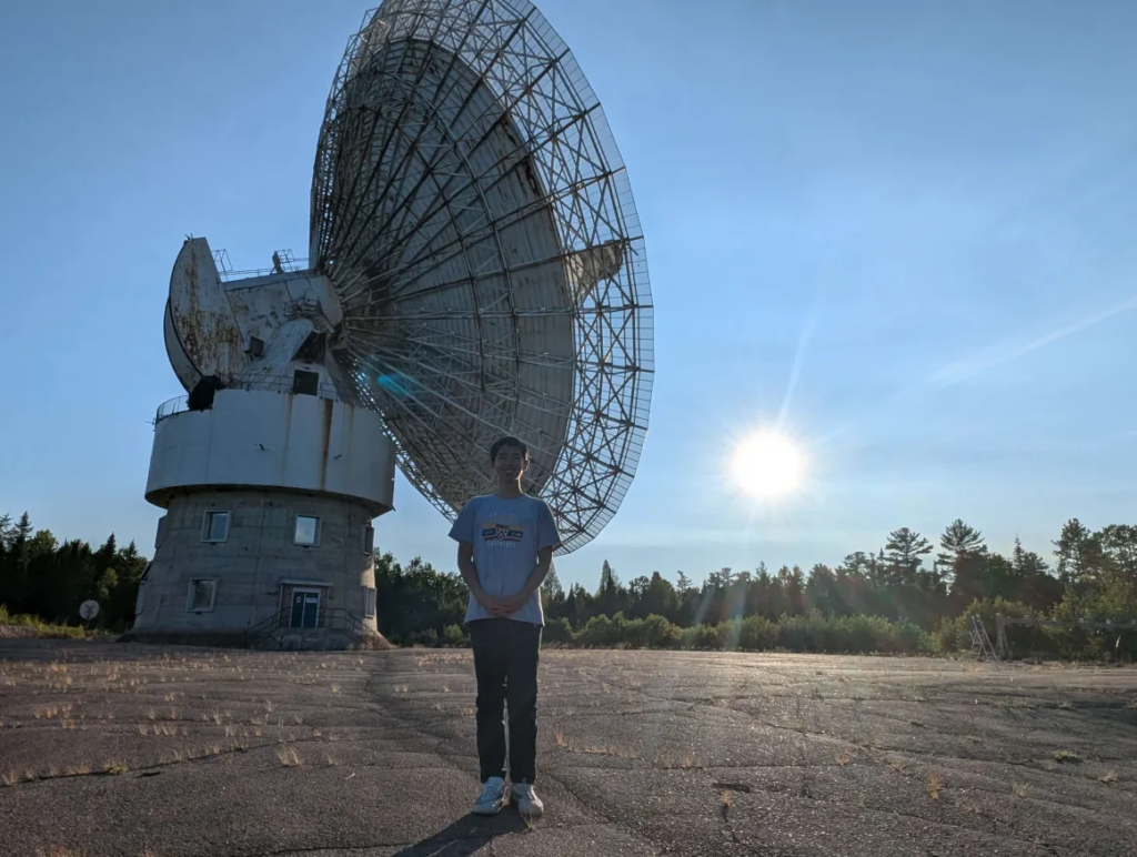
One can check out the website for ARO hosted by the space company Thoth technology. On Google Maps, one can also see a picture of it here (along with the LPDA in the top right):

ARO itself is a radio telescope with a \(46\) meter diameter dish. However, my main work in this project was not with the telescope itself, but rather a log-periodic dipole array (LPDA) nearby consisting of \(8\) antenna feeds sitting on a wire mesh to shield from RFI from the Earth.

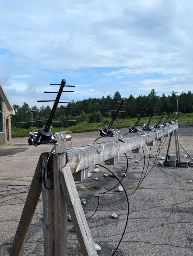
Radio waves from pulsars, from fast radio bursts, and (unfortunately) from terrestrial radiofrequency interference (RFI), of various frequencies \(f\) and from various directions \(\hat{\textbf n}\) are constantly bombarding the LPDA, inducing complicated AC voltages \(V_j(t)\) in each of the \(j=1,2,…,8\) LPDA antennas (part of why the \(V_j(t)\) are complicated is because of the anisotropic radiation pattern \(A(f,\hat{\textbf n})\) of the LPDA in both \(f\) and \(\hat{\textbf n}\)). For radio waves from pulsars and fast radio bursts in particular, they have travelled millions of light years to reach the LPDA, and are therefore very weak signals. For this reason, the AC voltages in the LPDA antennas are first fed as inputs into an amplifier (so-called “pre-amps”) shielded in an RFI Faraday cage (indeed, one can see them in the picture of the LPDA above where they are mounted by zip ties underneath the wooden beam holding the LPDA antennas). The output of these amplified signals then travel down long coaxial cables (pros: high-bandwidth in the data communication sense, built-in RFI shielding, weather-resistant, cheaper than fiber optic cables, low attenuation rates, etc.) into a basement area containing all the ARO computers.

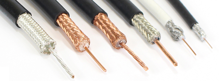
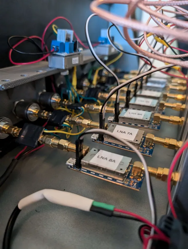
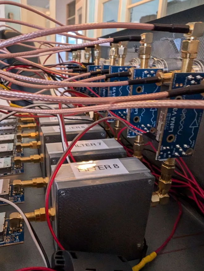
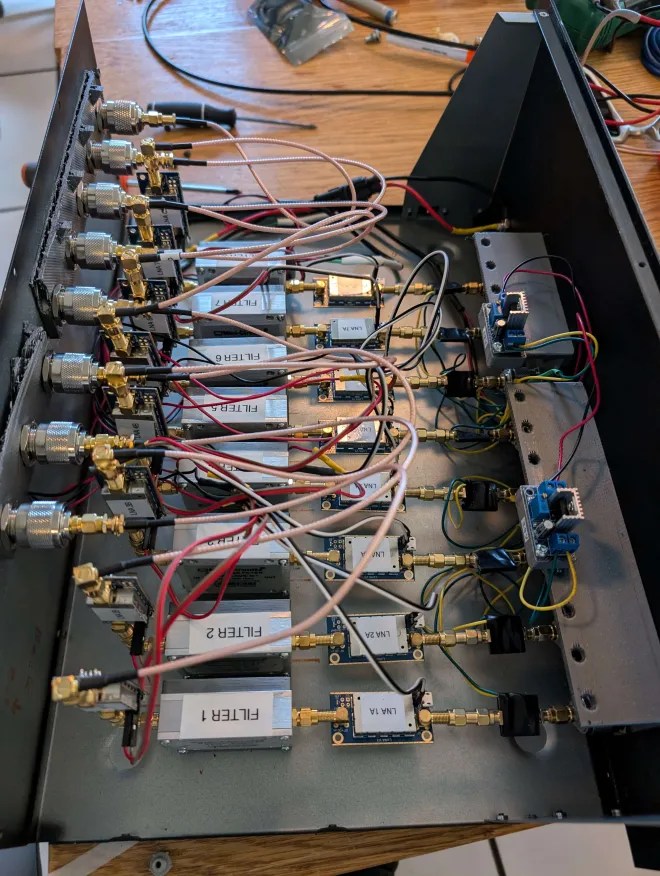
More precisely, these \(8\) coaxial cables are then fed (via \(N\) connectors) as inputs into two further stages (“stage-2” and “stage-3”) of amplification (using some low-noise amplifiers or LNAs from Amazon) and bandpass filtering with bandpass \(f\in[400,800]\text{ MHz}\) (from Mini-Circuits). I was told that the reason for this choice is because the CHIME telescope in British Columbia analyzes the same band of frequencies. These LNAs need to be powered with a \(6\text{ V}\) external DC voltage source. The \(8\) first-stage pre-amps also need power (but only \(3.3\text{ V}\)), so a \(3.3\text{ V}\) voltage regulator is used to step down the \(6\text{ V}\to 3.3\text{ V}\) and a set of \(8\) bias-tees are used to inject this \(3.3\text{ V}\) DC back down the coaxial cable (from where the RF signals are coming from) to those pre-amps outside the ARO computer room, thereby allowing them to be powered entirely from within the ARO computer room. This entire circuit is enclosed in a large metal black box acting as an RFI Faraday cage which I helped to install during my visit at ARO:

Additional \(N\)-connector coaxial cables would take the output from this whole process (which by the way is still what engineers call an analog signal, i.e. the kind that appeals to physicists and calculus-lovers) and transmit it down to an field-programmable gate array (FPGA) box which first performs digitization (i.e. the usual sampling and quantization steps of an ADC) and computes the discrete Fourier transform of the resultant digitized voltage signals. This is then called raw baseband data and essentially consists of long sequences of bits which are stored on one of the ARO computers called cloyd (named after the cartoon character from the 1950’s Rocky & Bullwinkle Show).