
Problem: Explain what the “nearly” in “nearly free electrons” means precisely.
Solution: It means the potential \(V\) experienced by the electrons is assumed to be weak in comparison to their kinetic energy \(V\ll T\) (in addition to being weak, it is also the case that the potential \(V\) is assumed to be periodic, though that’s not really conveyed by “nearly”). Immediately, the weak hypothesis on \(V\) implies it may be treated as a perturbation on \(T\) which is convenient because the simple kinetic Hamiltonian \(H=T\) has the familiar plane wave eigenstates \(|\mathbf k\rangle\) with energy eigenvalues \(E(\mathbf k)=\hbar^2|\mathbf k|^2/2m\).
Problem: Let \(\Lambda\) be a lattice in \(\mathbf R^d\), and let \(V(\mathbf x)\) be a weak \(\Lambda\)-periodic potential generated by some motif of atoms/ions present at each lattice point in \(\Lambda\). Within the nearly free electron model, explain qualitatively how the isotropic free electron dispersion \(E(\mathbf k)=\hbar^2|\mathbf k|^2/2m\) develops a discontinuity \(\Delta E_{\partial T^d}(\mathbf k)\) (called a band gap) on the boundary \(\mathbf k\in\partial T^d\) of the Brillouin zone \(T^d\).
Solution: A \(\Lambda\)-periodic function admits a Fourier series:
\[V(\mathbf x)=\frac{1}{|V_p|}\sum_{\mathbf k\in\Lambda^*}V_{V_p}(\mathbf k)e^{i\mathbf k\cdot\mathbf x}\]
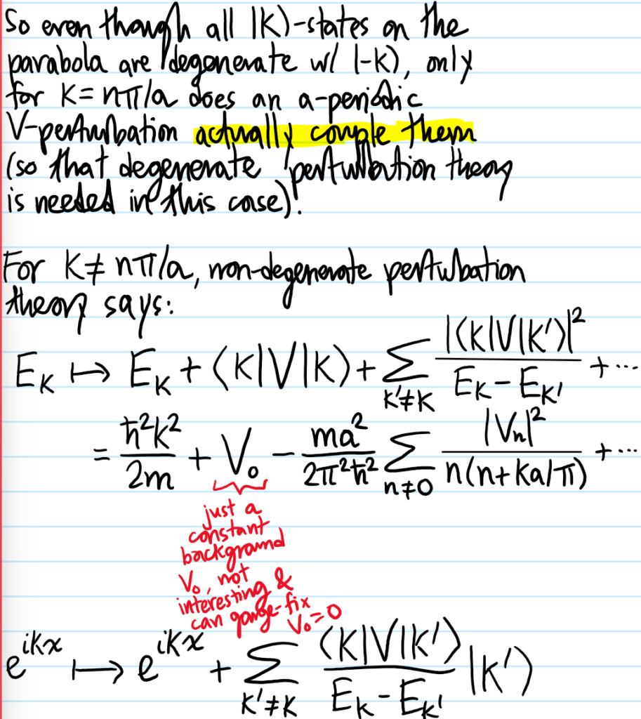
where the Fourier coefficients are determined by the structure factor of the potential \(V_{V_p}(\mathbf k)=\int_{V_p}d^d\mathbf xe^{-i\mathbf k\cdot\mathbf x}V(\mathbf x)\) with respect to a primitive cell \(V_p\) of volume \(|V_p||T^d|=(2\pi)^d\). If two plane wave states \(|\mathbf k\rangle,|\mathbf k’\rangle\) lie on the same sphere \(E(\mathbf k)=E(\mathbf k’)\) in \(\mathbf k\)-space, then degenerate perturbation theory is required iff the potential \(\langle\mathbf k’|V(\mathbf x)|\mathbf k\rangle\neq 0\) couples them:
\[\langle\mathbf k’|V(\mathbf x)|\mathbf k\rangle=|\mathbf T^d|V_{V_p}(\mathbf k’-\mathbf k)\sum_{\Delta\mathbf k\in\Lambda^*}\delta^d(\mathbf k’-\mathbf k-\Delta\mathbf k)\]
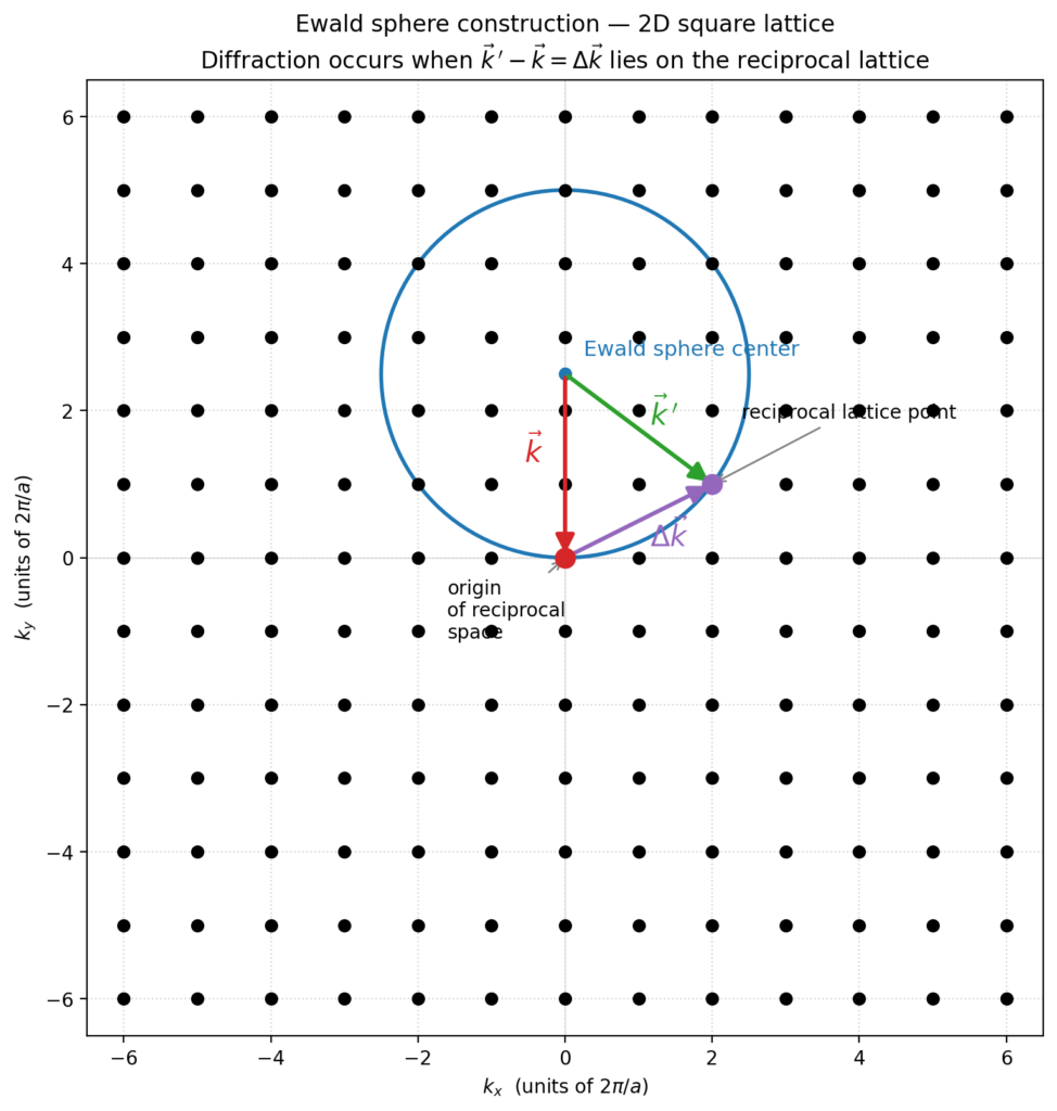
Thus, \(\langle\mathbf k’|V(\mathbf x)|\mathbf k\rangle\neq 0\Leftrightarrow\mathbf k’-\mathbf k\in\Lambda^*\) which is sometimes visualized in \(d=2,3\) via the Ewald sphere construction:
Furthermore, in practice Born-von Karman quantization of \(\mathbf k\)-space due to a finite real space volume means that the Dirac comb can be replaced by a “Kronecker comb” that leads directly to the Fourier coefficient:
\[\langle\mathbf k’|V(\mathbf x)|\mathbf k\rangle=V_{V_p}(\mathbf k’-\mathbf k)/|V_p|\]
Thus, although in the Brillouin zone interior \(\text{int}(T^d)\) there exist uncountably many degenerate spheres \(S^{d-1}(k)\), it is only for radii \(k>0\) intersecting the Brillouin zone boundary \(S^{d-1}(k)\cap\partial T^d\neq\emptyset\) that there is a hope of two wavevectors \(\mathbf k,\mathbf k’\in S^{d-1}(k)\cap\partial T^d\) differing by \(\mathbf k’-\mathbf k\in\Lambda^*\) simply because of how \(T^d\) is defined as the Wigner-Seitz cell of \(\Lambda^*\).
Problem: Flesh out completely all the implications of the \(d=1\) nearly free electron model.
Solution:
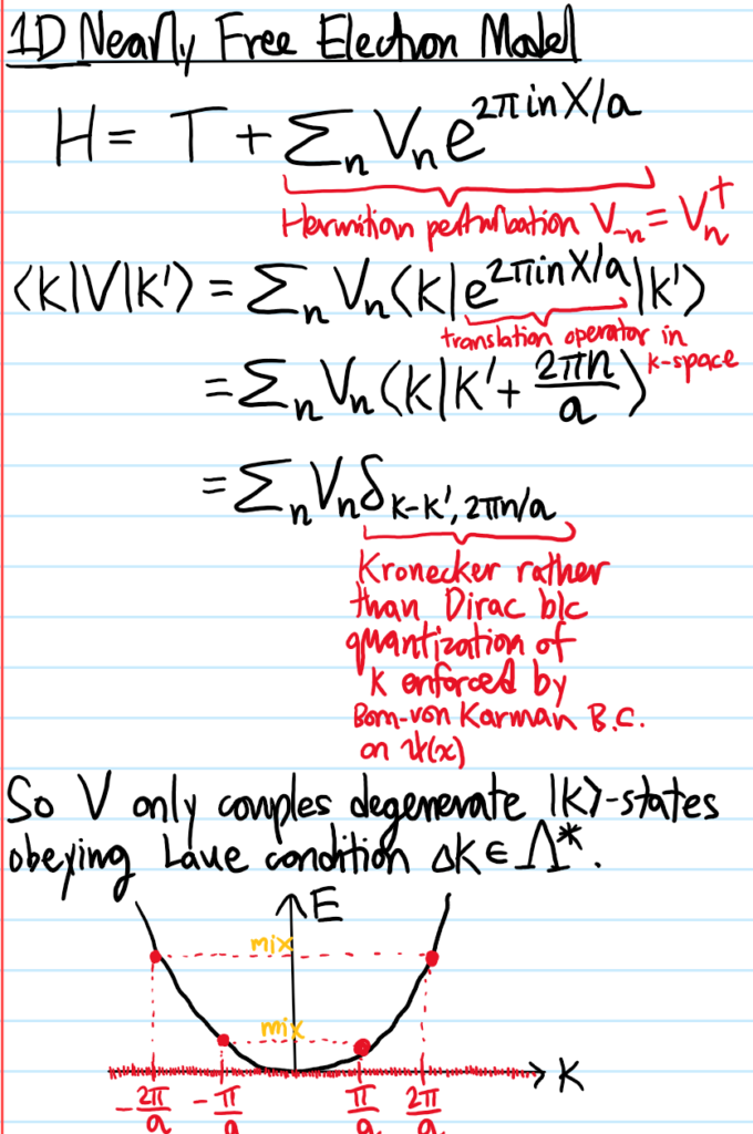
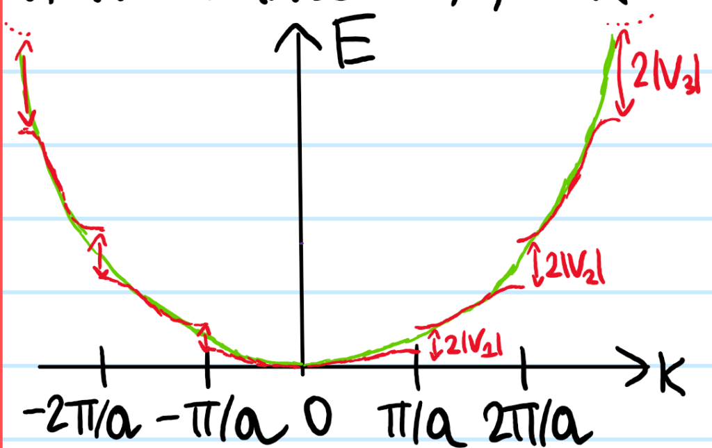
In the \(1\)D extended zone scheme, the band structure (a butchering of the free particle parabolic dispersion) looks like:
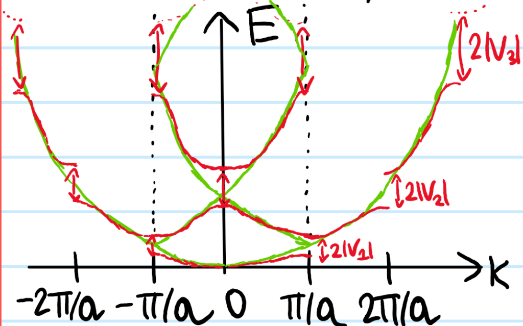
or in the \(1\)D reduced zone scheme:
Problem: Comment on the group velocity and effective mass behaviour of this band structure.
Solution: The group velocity of electron wavepacket provides \(1^{\text{st}}\) derivative information about the dispersion (here \(p=\hbar k\)):
\[v:=\frac{\partial E}{\partial p}\]
One heuristic justification for the electron group velocity flattening out \(v\to 0\) at zone boundaries \(k=n\pi/a\) is that this ensures upon backfolding into the \(1^{\text{st}}\) Brillouin zone in the reduced zone scheme that the group velocity \(v=v(k)\) remains a continuous function of \(k\) at \(k=n\pi/a\).
Meanwhile, the effective mass provides \(2^{\text{nd}}\) derivative information about the dispersion:
\[\frac{1}{m^*}=\frac{\partial^2 E}{\partial p^2}\]
(i.e. one can think of \(m^*\) as the radius of curvature at a point on the dispersion). For the electron it is positive near the bottom of a band but negative near the top, whereas it is the other way around for holes.
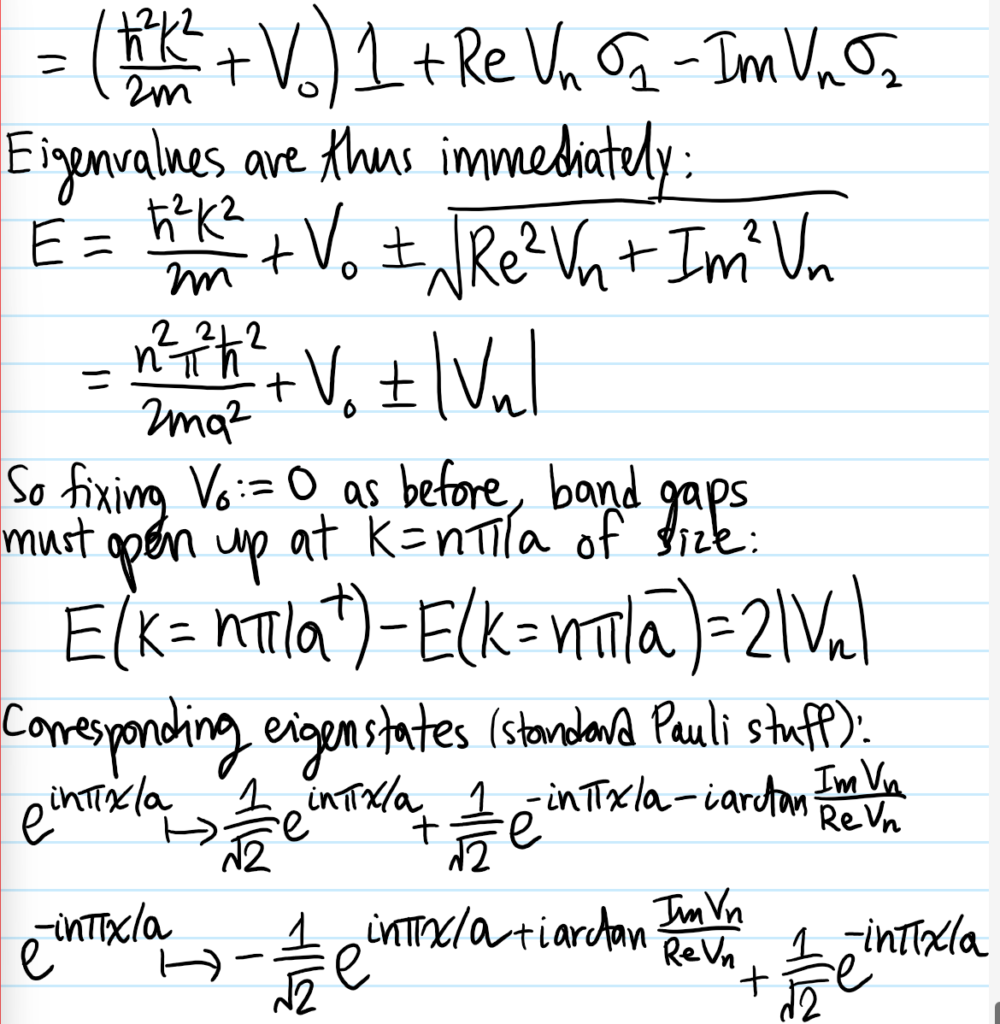
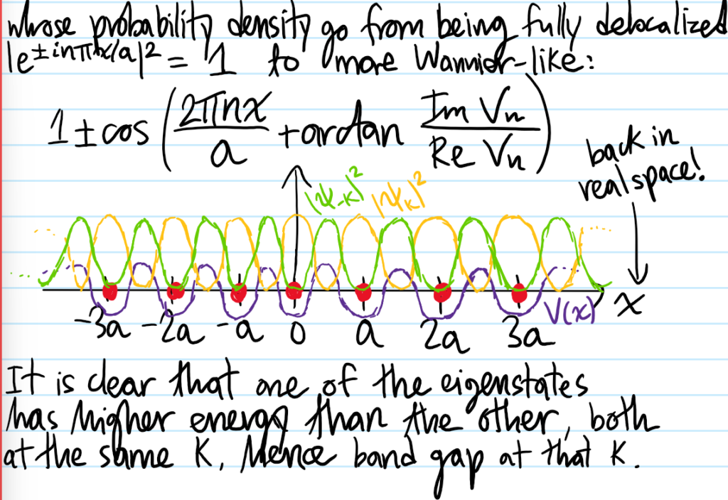
Problem: Let \(\Lambda\) be an arbitrary lattice in dimension \(d\), and let \(\mathbf k_0\in (T^d)^{(d-1)}\) be a wavevector on the Brillouin zone boundary such that it couples to only one other wavevector \(\mathbf k_0-\Delta\mathbf k\in (T^d)^{(d-1)}\) for \(\Delta\mathbf k\in\Lambda^*\) and no other \((d-1)\)-skeleton wavevectors in the CW complex \((T^d)^{(d-1)}\). In that case, show that the nearly free electron dispersion relation in a neighbourhood of \(\mathbf k=\mathbf k_0\) is the sum of non-relativistic and “relativistic” contributions:
\[E_{\pm}(\mathbf k)=\varepsilon_{\mathbf k-\Delta\mathbf k/2}+\varepsilon_{\Delta \mathbf k/2}+V_{\mathbf 0}\pm\sqrt{((\mathbf p-\mathbf p_0)\cdot\mathbf v_0)^2+|V_{\Delta\mathbf k}|^2}\]
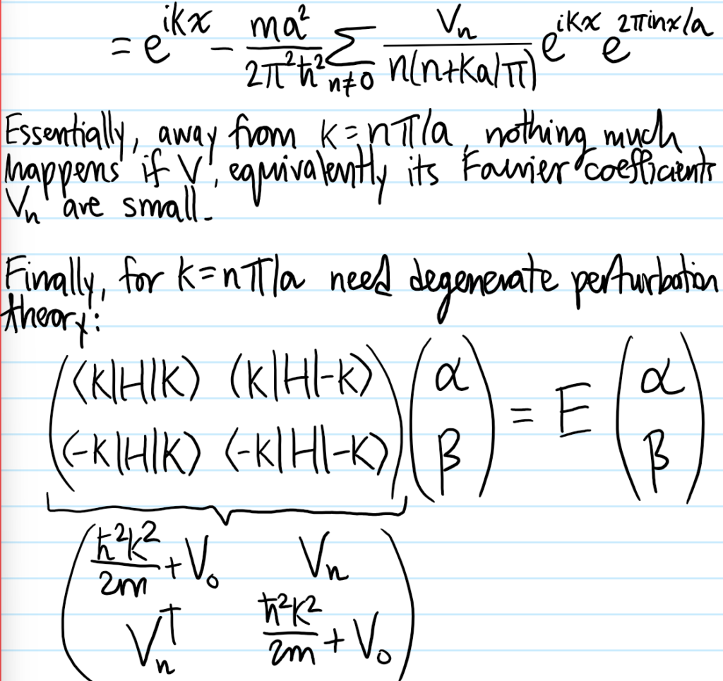
Solution: The \(2\times 2\) Hamiltonian matrix restricted to the ~degenerate subspace \(\text{span}_{\mathbf C}|\mathbf k\rangle,|\mathbf k-\Delta\mathbf k\rangle\) is:
\[H=\begin{pmatrix}\varepsilon_{\mathbf k}+V_{\mathbf 0}&V_{\Delta\mathbf k}\\V^{\dagger}_{\Delta\mathbf k}&\varepsilon_{\mathbf k-\Delta\mathbf k}+V_{\mathbf 0}\end{pmatrix}\]
Writing \(\mathbf k=\mathbf k_0+\delta\mathbf k\) and invoking \(\varepsilon_{\mathbf k_0-\Delta\mathbf k}=\varepsilon_{\mathbf k_0}\Leftrightarrow \mathbf k_0\cdot\Delta\mathbf k=|\Delta\mathbf k|^2/2\), one can massage \(H\) into the form:
\[H=\left(\varepsilon_{\mathbf k-\Delta\mathbf k/2}+\varepsilon_{\Delta\mathbf k/2}+V_{\mathbf 0}\right)1-\mu_B\boldsymbol{\sigma}\cdot\mathbf B\]
with effective magnetic field \(\mathbf B=-\mu_B^{-1}(\text{Re}V_{\Delta\mathbf k},-\text{Im}V_{\Delta\mathbf k},(\mathbf p-\mathbf p_0)\cdot\mathbf v_0)\). Standard properties of Pauli matrices then yields the desired spectrum. In particular, the group velocity vector field and effective mass tensor field are given by:
\[\frac{\partial E_{\pm}}{\partial\mathbf p}=\mathbf v-\frac{\Delta\mathbf v}{2}\pm\frac{(\mathbf p-\mathbf p_0)\cdot\mathbf v_0}{\sqrt{((\mathbf p-\mathbf p_0)\cdot\mathbf v_0)^2+|V_{\Delta\mathbf k}|^2}}\mathbf v_0\]
\[\frac{1}{m^*_{\pm}(\mathbf k)}=\frac{\partial^2 E_{\pm}}{\partial\mathbf p^{\otimes 2}}=\frac{1}{m}\pm\frac{|V_{\Delta\mathbf k}|^2}{(((\mathbf p-\mathbf p_0)\cdot\mathbf v_0)^2+|V_{\Delta\mathbf k}|^2)^{3/2}}\mathbf v^{\otimes 2}_0\]
with particular values:
\[\frac{\partial E_{\pm}}{\partial(\mathbf p=\mathbf p_0)}=\mathbf v_0-\frac{\Delta\mathbf v}{2}\]
\[\frac{1}{m^*_{\pm}(\mathbf k_0)}=\frac{1}{m}\pm\frac{\mathbf v_0^{\otimes 2}}{|V_{\Delta\mathbf k}|}\]
Problem: Consider a \(d=1\) linear lattice \(\Lambda_a\) with single-atom motifs spaced periodically a distance \(a\) apart, and suppose each atom is monovalent \(z=1\). Although standard band structure theory predicts that the first energy band will thus be half-filled and the material a metal as a result, explain why in practice (especially at sufficiently low temperatures) this is actually not the case.
Solution: Peierls instability/metal-to-insulator transition.
Digression on Floquet Theory
There is another, more abstract way to qualitatively see why a periodic potential \(V(x+\Delta x)=V(x)\) gives rise to Brillouin zones and energy bands.
Consider an \(N\)-dimensional linear dynamical system \(\dot{\textbf x}(t)=A(t)\textbf x(t)\) where \(A(t)\) can be time-dependent. In general, one expects this to have \(N\) linearly independent solutions \(\textbf x_1(t),\textbf x_2(t),…,\textbf x_N(t)\). A fundamental matrix solution \(X(t)\) to the linear dynamical system is any \(N\times N\) matrix comprised of a basis of \(N\) such linearly independent solutions \(X(t)=\left(\textbf x_1(t),\textbf x_2(t),…,\textbf x_N(t)\right)\), so in other words the linear independence implies that \(X(t)\in GL_N(\textbf R)\) is invertible \(\det X(t)\neq 0\) at all times \(t\in\textbf R\). Think of the fundamental matrix solution \(X(t)\) as an \(N\)-dimensional parallelotope evolving in time \(t\). It can be checked that any fundamental matrix solution \(\dot{X}(t)=A(t)X(t)\) satisfies the same system of ODEs, and that any individual solution \(\textbf x(t)\) must lie in the column space \(\textbf x(t)\in\text{span}_{\textbf R}(\textbf x_1(t),…,\textbf x_N(t))\) of any fundamental matrix solution \(X(t)\) (indeed, this is why it’s called “fundamental” because it provides a basis for the entire solution space of the linear dynamical system). Thus, \(\textbf x(t)=X(t)X^{-1}(0)\textbf x(0)\). If \(X(0)=1_{N\times N}\), then \(X(t)\) is called a principal fundamental matrix solution and in that case we just have \(\textbf x(t)=X(t)\textbf x(0)\). Thus, the principal fundamental matrix solution plays a role analogous to the time evolution operator \(U(t)\) in quantum mechanics, evolving the initial state of a system through time \(t\).
Floquet theory is interested in a special case of the setup above, namely when \(A(t+T)=A(t)\) is a \(T\)-periodic matrix. In this case, it turns out that the solutions \(\textbf x(t)\) themselves will not necessarily be \(T\)-periodic (or periodic at all for that matter), but will nonetheless take on a much simpler form than the otherwise unenlightening time-ordered exponential solution \(\textbf x(t)=\mathcal Te^{\int_0^tA(t’)dt’}\textbf x(0)\) as a Dyson series. What’s that simplification? Let me spoil it first, then prove it afterwards. Recall that I just said \(\textbf x(t)\) won’t necessarily be periodic. But that should feel pretty strange since \(A(t)\) is by assumption \(T\)-periodic so surely \(\textbf x(t)\) should inherit something from this. And that’s exactly the essence of Floquet’s theorem, namely that although \(\textbf x(t)\) itself need not be periodic, its time evolution can always be factorized into a \(T\)-periodic \(N\times N\) matrix \(X_A(t)\) (with the subscript \(A\) to suggest that it inherits its \(T\)-periodicity \(X_A(t+T)=X_A(t)\) from the \(T\)-periodicity of the matrix \(A(t)\)) modulated by an exponential growth/decay or oscillatory “envelope” \(e^{\Lambda t}\) for some time-independent \(N\times N\) (possibly complex) matrix \(\Lambda\in\textbf C^{N\times N}\). In other words, one has the ansatz:
\[\textbf x(t)=X_A(t)e^{\Lambda t}\textbf x(0)\]
To prove Floquet’s theorem, we first ask: although \(\textbf x(t+T)\neq\textbf x(t)\) need not be periodic, how are \(\textbf x(t+T)\) and \(\textbf x(t)\) related to each other? Clearly by a simple \(T\)-time translation \(\textbf x(t+T)=X(t+T)X^{-1}(t)\textbf x(t)\). It makes sense then to focus on understanding these fundamental matrix solutions \(X(t)\) better.
The first key result of Floquet theory is that the time evolution of any fundamental matrix solution \(X(t)\) across a period \(T\) behaves multiplicatively \(X(t+T)=X(t)\tilde X_T\) where the \(N\times N\) monodromy matrix \(\tilde X_T=X^{-1}(t)X(t+T)\) is a conserved quantity of any \(T\)-periodic linear dynamical system:
\[\dot{\tilde X}_T=-X^{-1}(t)A(t)X(t+T)+X^{-1}(t)A(t+T)X(t+T)=0\]
It is thus common to initialize the monodromy matrix \(\tilde X_T=X^{-1}(0)X(T)\) and write \(X(t+T)=X(t)X^{-1}(0)X(T)\). After \(n\) periods elapse we have \(X(t+nT)=X(t)\tilde X_T^n\) so as a corollary for instance the hypervolume \(\det X(t)\) of the parallelotope grows stroboscopically in time \(t\) as a geometric sequence \(\det X(t+nT)=(\det \tilde X_T)^n\det X(t)\). Indeed, using Jacobi’s formula one can check that \(\dot{\det}X(t)=\det A(t)\det X(t)\) so \(\det X(t)=e^{\int_0^tA(t’)dt’}\det X(0)\) is consistent with \(X(t+T)=X(t)\tilde X_T\) provided the monodromy matrix \(\tilde X_T\) and \(A(t)\) are related by \(\det\tilde X_T=e^{\int_0^T\text{Tr} A(t)dt}\) (despite the suggestion, note that in general \(\tilde X_T\neq e^{\int_0^T A(t)dt}\)! Everything would be simpler if this were true but alas it isn’t).
It is therefore intuitively clear that the behavior/stability of any periodic linear dynamical system is sensitive to its monodromy matrix \(\tilde X_T\), specifically whether it “blows up” or “decays” exponentially or oscillates (as would have been one’s first instinct given the periodicity \(A(t+T)=A(t)\) of \(A\))! More precisely, to understand the behavior of powers \(\tilde X_T^n\) of a matrix, it is always a good idea to diagonalize it (a subtle but important property of the monodromy matrix \(\tilde X_T\) proven on page \(52\) here is that although it depends on the choice of fundamental matrix solution \(X(t)\) used to construct it, it will be similar to any other monodromy matrix \(\tilde X’_T\) constructed from any other fundamental matrix solution \(X'(t)\); thus, the eigenvalues of the monodromy matrix \(\tilde X_T\) are properties only of the linear, periodic dynamical system \(\dot X=AX\) and therefore are rightfully called its characteristic multipliers).
Since \(\tilde X_T\in GL_N(\textbf R)\), these characteristic multipliers must be non-zero, and so all such characteristic multipliers can be written as \(e^{\lambda T}\) for some \(\lambda\in\textbf C\) called its characteristic exponent. Although the imaginary part \(\Im\lambda\) of such a characteristic exponent is not unique \(e^{(\lambda+2\pi i/T)T}=e^{\lambda T}\), the real part \(\Re\lambda\) is unique and physically meaningful, being given the name Lyapunov exponent. Specifically, it is clear that if a solution \(\textbf x(t)\) happens to initialize on \(\textbf x(0)=X(0)\tilde{\textbf x}\) where \(\tilde X_T\tilde{\textbf x}=e^{\lambda T}\tilde{\textbf x}\) is an eigenvector of the monodromy matrix \(\tilde X_T\), then one can check that such a solution \(\textbf x(t+T)=e^{\lambda T}\textbf x(t)\) evolves multiplicatively in an analogous manner to the fundamental matrix solution earlier. In particular, if one replaces this \(\textbf x(t)\mapsto \textbf x_A(t):=e^{-\lambda t}\textbf x(t)\), then clearly this new trajectory (but no longer a solution!) \(\textbf x_A(t)\) is \(T\)-periodic \(\textbf x_A(t+T)=e^{-\lambda t}e^{-\lambda T}\textbf x(t+T)=e^{-\lambda t}e^{-\lambda T}e^{\lambda T}\textbf x(t)=e^{-\lambda t}\textbf x(t)=\textbf x_A(t)\). Thus, one can isolate the form of this “eigentrajectory” as \(\textbf x(t)=e^{\lambda t}\textbf x_A(t)\). For \(\Re \lambda<0\) we have \(\lim_{t\to\infty}\textbf x(t)=\textbf 0\), for \(\Re \lambda>0\) we have \(\lim_{t\to\infty}\textbf x(t)=\boldsymbol{\infty}\) while for \(\Re \lambda=0\) the eigentrajectory \(\textbf x(t)\) is in general pseudoperiodic in that it ends up at the same distance \(|\textbf x(t+T)|=|\textbf x(t)|\) (but not necessarily the same point) away from the origin after each period \(t\mapsto t+T\). These criteria emphasize the role played by the Lyapunov exponent \(\Re\lambda\) in the analysis of stability. By lining up \(N\) such linearly independent eigentrajectories (we’ll assume that the monodromy matrix \(\tilde X_T\) is diagonalizable), it follows that any fundamental matrix solution \(X(t)\) admits a so-called Floquet normal form \(X(t)=X_{A}(t)e^{\Lambda t}\) where \(X_A(t+T)=X_A(t)\) inherits the \(T\)-periodicity of \(A\) and \(\Lambda\) is a time-independent \(N\times N\) matrix. This therefore proves Floquet’s theorem!
Connection to Periodic Potentials in Quantum Mechanics
Define \(\boldsymbol{\phi}(x):=(\psi(x),\psi'(x))^T\) so that the one-dimensional second-order Schrodinger equation reduces to the first-order linear system:
\[\boldsymbol{\phi}'(x)=A(x)\boldsymbol{\phi}(x)\]
where \(A(x)=\begin{pmatrix}0&1\\2m(V(x)-E)/\hbar^2 & 0\end{pmatrix}\) is \(\Delta x\)-periodic \(A(x+\Delta x)=A(x)\) by virtue of the \(\Delta x\)-periodicity of the potential \(V(x)\) itself. Now notice that clearly \(\text{Tr} A(x)=0+0=0\), so it follows from the earlier general Floquet theory results that \(\det\tilde \Phi_{\Delta x}=1\) where \(\tilde \Phi_{\Delta x}\) is the monodromy matrix of the periodic quantum system. This means that its two eigenvalues \(\varphi_{\pm}\) are given by:
\[\varphi_{\pm}=\frac{\text{Tr}\tilde \Phi_{\Delta x}}{2}\pm\sqrt{\frac{\text{Tr}^2\tilde \Phi_{\Delta x}}{4}-1}\]
Thus, when \(\text{Tr}\tilde \Phi_{\Delta x}<-2\) or \(\text{Tr}\tilde \Phi_{\Delta x}>2\), both \(\phi_{\pm}>0\) are real and positive, indicating a spatially unstable wavefunction \(\psi(x)\) that diverges in a non-normalizable manner as \(x\to\pm\infty\). Therefore, this is saying that there do not exist \(H\)-eigenstates with energy \(E\) such that the corresponding monodromy matrix \(\tilde \Phi_{\Delta x}=\tilde \Phi_{\Delta x}(E)\) has trace less than \(-2\) or greater than \(2\). These are the band gaps between the various energy bands! Of course then, on the other hand when \(\text{Tr}\tilde \Phi_{\Delta x}\in(-2,2)\) is in the zone of spatial stability (aka \(L^2\)-normalizability), these are associated with the energy bands! Finally, exactly when \(\text{Tr}\tilde \Phi_{\Delta x}=\pm 2\) is where one reaches the boundaries separating various Brillouin zones! Admittedly this Floquet analysis is a bit abstract and handwavy but I still think it’s a nice alternative perspective to the more concrete nearly-free electron model.
If we let \(\Phi(x)=\begin{pmatrix}\psi_1(x) & \psi_2(x) \\ \psi’_1(x) & \psi’_2(x)\end{pmatrix}\) be a fundamental matrix solution, then of course \(\det\Phi(x)\) is the usual constant Wronskian of two wavefunctions \(\psi_1(x),\psi_2(x)\), and Floquet’s theorem allows us to write \(\Phi(x)=\Phi_V(x)e^{\Lambda x}\) for a \(\Delta x\)-periodic \(2\times 2\) matrix \(\Phi_V(x+\Delta x)=\Phi_V(x)\) whose \(\Delta x\)-periodicity is inherited from the \(\Delta x\)-periodicity of the potential \(V(x)\). This leads to Bloch’s theorem (in one dimension), namely that there exists a crystal momentum \(k\in[-\pi/\Delta x,\pi/\Delta x]\) in the first Brillouin zone is given by the Bloch state \(\psi_{k}(x)=e^{ikx}\phi_k(x)\).