
Problem: What is the position space wavefunction \(\psi(\textbf x)\) of a photon in a box of volume \(V=L^3\) whose opposite faces are subject to periodic boundary conditions? What about reflecting boundary conditions?
Solution: With periodic boundary conditions, the wavefunctions are travelling plane waves:
\[\psi(\textbf x)\sim e^{i\textbf k\cdot\textbf x}\]
where \(\textbf k\in\frac{2\pi}{L}\textbf Z^3\).
With reflecting boundary conditions (e.g. ideal conductor surfaces), wavefunctions are standing waves (suitable superpositions of travelling plane waves):
\[\psi(\textbf x)\sim\sin(k_xx)\sin(k_yy)\sin(k_zz)\]
where \(k_x,k_y,k_z\in \frac{\pi}{L}\textbf Z^+\) (the \(\textbf Z^+\) here rather than a \(\textbf Z\) restricts to the first octant in \(\textbf k\)-space because e.g. \(\sin(-k_xx)=-\sin(k_xx)\) is a physically equivalent state.
(if one wants to normalize these wavefunctions, then in the former case it’s \(1/\sqrt{V}\), in the latter case it’s \(\sqrt{8/V}\)).
Problem: Write down the Planck distribution \(\mathcal E_{\omega}\).
Solution: Keeping in mind \(\omega=ck\):
\[\mathcal E_{\omega}=2\times\frac{V}{(2\pi)^3}4\pi k^2\frac{\hbar\omega}{e^{\beta\hbar\omega}-1}\]
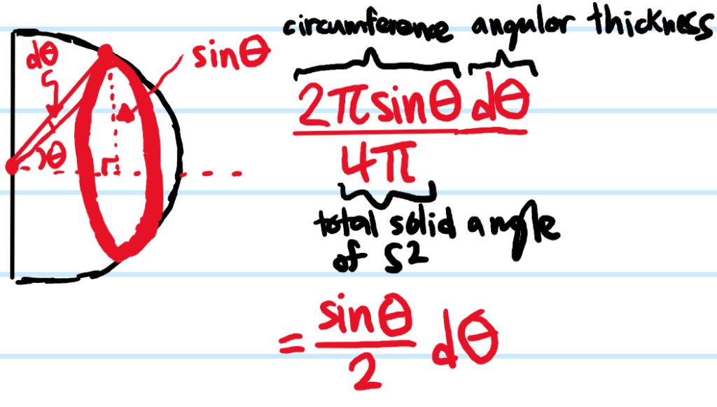
Problem: Assuming an isotropic photon gas, find an expression for the irradiance density \(I(\omega)\) incident normally on a face of the cavity.
Solution: Letting the unit normal to the face be \(\hat{\textbf z}\), this is given by the hemispherical expectation of the Poynting vector projection along \(\hat{\textbf z}\):
\[I(\omega)d\omega=\langle\textbf S_{\omega}(\hat{\textbf n})\cdot\hat{\textbf z}\rangle_{\hat{\textbf n}\in S^2/2}\]
where the Poynting vector for electromagnetic waves (or photons) of frequency \(\omega\) travelling in direction \(\hat{\textbf n}\) is:
\[\textbf S_{\omega}(\hat{\textbf n})=\mathcal E_{\omega}d\omega c\hat{\textbf n}\]
So, using an isotropic distribution \(p(\hat{\textbf n})=1/4\pi\):
\[I(\omega)=\mathcal E_{\omega}c\int_{S^2/2} d^2\hat{\textbf n}p(\hat{\textbf n})\hat{\textbf n}\cdot\hat{\textbf z}\]
\[=\mathcal E_{\omega}c\int_0^1 d\cos\theta\int_0^{2\pi}d\phi \frac{1}{4\pi}\cos\theta\]
\[=\frac{\mathcal E_{\omega} c}{4}\]
Problem: Derive the Stefan-Boltzmann law.
Solution: Integrate the irradiance density over all \(\omega\in(0,\infty)\):
\[\frac{P}{A}=\int_0^{\infty}d\omega I(\omega)=\sigma T^4\]
where \(\sigma:=\frac{\pi^2k_B^4}{60c^2\hbar^3}\).
Problem: So the Stefan-Boltzmann law says that as an object gets hotter (avoid using the term blackbody), it emits more energy in proportion to \(T^4\); but how much of this effect is due to the energy of the individual photons actually increasing and how much is due to the fact that it’s emitting more photons?
Solution: \(4=1+3\), where the \(1\) is the energy increase of each photon, while the \(3\) is the increase in the number of photons emitted (thus, it is clear what the dominant effect is).
Mystery (Why This Derivation Fails?)
The canonical partition function for the photon gas is actually (remembering also the \(1/N!\) Gibbs factor):
\[Z=\sum_{N=0}^{\infty}\frac{1}{N!}\sum_{(\textbf n_1,\textbf n_2,…,\textbf n_N)\in\textbf Z^{3N}}\sum_{(|\psi_1\rangle,|\psi_2\rangle,…,|\psi_N\rangle)\in\{|0\rangle,|1\rangle\}^N}e^{-\beta E_{(\textbf n_1,\textbf n_2,…,\textbf n_N)}}\]
where the total energy of the photon gas in that particular microstate is degenerate with respect to their polarizations, instead depending only on the momenta \(E_{(\textbf n_1,\textbf n_2,…,\textbf n_N)}=\frac{2\pi\hbar c}{L}\sum_{i=1}^N|\textbf n_i|\). As a result, we can move the exponential outside the sum over polarization states \(\sum_{(|\psi_1\rangle,|\psi_2\rangle,…,|\psi_N\rangle)\in\{|0\rangle,|1\rangle\}^N}1=2^N\). We can also convert the exponential of the series of energies into a product \(e^{-\beta E_{(\textbf n_1,\textbf n_2,…,\textbf n_N)}}=\prod_{i=1}^Ne^{-2\pi\beta\hbar c|\textbf n_i|/L}\).
The series of products \(\sum_{(\textbf n_1,\textbf n_2,…,\textbf n_N)\in\textbf Z^{3N}}\prod_{i=1}^Ne^{-2\pi\beta\hbar c|\textbf n_i|/L}\) is tricky to calculate but can be accurately estimated with the aid of a useful approximation.
Digression on the Euler-Maclaurin Summation Formula
The Euler-Maclaurin summation formula asserts that, for any smooth function \(f\in C^{\infty}(\textbf R\to\textbf C)\), if we sum the values of \(f\) evaluated on a bunch of consecutive integers \(\sum_{n=a}^bf(n)\) with \(a,b\in\textbf Z\cup\{-\infty,\infty\}\), then this is often well-approximated by the integral \(\int_a^bf(n)dn\) of the function \(f\) on the interval \([a,b]\), treating \(n\) as though it were a continuous variable \(n\in\textbf R\) rather than an integer \(n\in\textbf Z\) (of course this is a two-way street, meaning that many integrals can also be approximated by suitable series). The canonical example of the Euler-Maclaurin summation formula concerns the harmonic series \(f(n)=1/n\), with the following diagram given to rationalize why the Euler-Maclaurin approximation should be a good approximation:

However, the full Euler-Maclaurin formula also acknowledges that the approximation is imperfect by explicitly giving a formula for the error/discrepancy between the series and its integral approximation:
\[\sum_{n=a}^bf(n)=\int_a^bf(n)dn+\frac{f(a)+f(b)}{2}+\sum_{n=1}^{\infty}\frac{B_{2n}}{(2n)!}\left(f^{[2n-1]}(b)-f^{[2n-1]}(a)\right)\]
where the asymptotic series on the right features the non-zero even Bernoulli numbers \(B_2=1/6,B_4=-1/30\), etc. This interesting sequence of rational numbers were historically first discovered in the context of Faulhaber’s formula \(1^p+2^p+…+n^p=\frac{1}{p+1}\left(B_0{{p+1}\choose{0}}n^{p+1}+B_1{{p+1}\choose{1}}n^{p}+…+B_p{{p+1}\choose{p}}n\right)\) for sums of powers, but arguably the real utility of the Bernoulli numbers lies in their appearance in the Euler-Maclaurin summation formula (indeed Faulhaber’s formula is just the special case of the Euler-Maclaurin summation formula with \(f(n)=n^p\)). The quickest way to compute these Bernoulli numbers is to use a Pascal-like triangle construction (details can be found in this paper of Kawasaki and Ohno). The idea is to first write down a couple terms of the harmonic sequence \(1, 1/2,1/3,…\) in the first row. Then, whereas in Pascal’s triangle one would compute the number “below” two numbers by simply adding them, here instead one first has to subtract the two (left number minus right number, or if you forget then bigger number minus smaller number to always obtain a positive difference), and then multiply the result by the denominator of whichever term in the original harmonic sequence \(1, 1/2,1/3,…\) lies on the same downward-sloping “diagonal column” so to speak. A picture is worth \(10^3\) words:
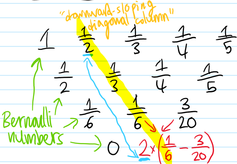
The Bernoulli numbers \(B_0=1,B_1=1/2,B_2=1/6\), etc. are then simply read off as the elements on the first (left-most) downward-sloping diagonal column (SHOULD INCLUDE SOME COMMENTS ABOUT WHEN EULER-MACLAURIN SUMMATION IS VALID AND RELATE IT TO THE STATISTICAL MECHANICAL APPLICATION FUNCTION WHICH IS EXPONENTIALLY DECAYING!).
Back to the Physics
All this is to say that we expect we can approximate the series of products earlier \(\sum_{(\textbf n_1,\textbf n_2,…,\textbf n_N)\in\textbf Z^{3N}}\prod_{i=1}^Ne^{-2\pi\beta\hbar c|\textbf n_i|/L}\) over the discrete lattice \(\textbf Z^{3N}\) by an integral over the smooth manifold \(\textbf R^{3N}\) instead, obtaining a \(3N\)-dimensional analog of the Euler-Maclaurin summation formula:
\[\sum_{(\textbf n_1,\textbf n_2,…,\textbf n_N)\in\textbf Z^{3N}}\prod_{i=1}^Ne^{-2\pi\beta\hbar c|\textbf n_i|/L}\approx \int_{(\textbf n_1,\textbf n_2,…,\textbf n_N)\in\textbf R^{3N}}\prod_{i=1}^Ne^{-2\pi\beta\hbar c|\textbf n_i|/L}d^3\textbf n_i\]
Notice that the \(N\) integrals for each photon completely decouple from each other (as expected because the photons are non-interacting):
\[\int_{(\textbf n_1,\textbf n_2,…,\textbf n_N)\in\textbf R^{3N}}\prod_{i=1}^Ne^{-2\pi\beta\hbar c|\textbf n_i|/L}d^3\textbf n_i=\prod_{i=1}^N\iiint_{\textbf n_i\in\textbf R^3}e^{-2\pi\beta\hbar c|\textbf n_i|/L}d^3\textbf n_i\]
Moreover, each of these integrals are identical (because each photon is an identical boson) so the product becomes an \(N\)-fold exponentiation:
\[\prod_{i=1}^N\iiint_{\textbf n_i\in\textbf R^3}e^{-2\pi\beta\hbar c|\textbf n_i|/L}d^3\textbf n_i=\left(\iiint_{\textbf n\in\textbf R^3}e^{-2\pi\beta\hbar c|\textbf n|/L}d^3\textbf n\right)^N\]
Expressing the volume element \(d^3\textbf n=4\pi|\textbf n|^2d|\textbf n|\) in spherical coordinates, the integral comes out as:
\[\iiint_{\textbf n\in\textbf R^3}e^{-2\pi\beta\hbar c|\textbf n|/L}d^3\textbf n=4\pi\int_0^{\infty}|\textbf n|^2e^{-2\pi\beta\hbar c|\textbf n|/L}d|\textbf n|=4\pi\left(\frac{L}{2\pi\beta\hbar c}\right)^3\Gamma(3)=\frac{V}{\pi^2\beta^3\hbar^3c^3}\]
So assembling everything together, the canonical partition function \(Z\) for the photon gas becomes:
\[Z=\sum_{N=0}^{\infty}\frac{(2V/\pi^2\beta^3\hbar^3c^3)^N}{N!}=e^{2V/\pi^2\beta^3\hbar^3c^3}\]
Unfortunately, I believe the correct answer is actually \(Z=e^{\pi^2 V/45\beta^3\hbar^3c^3}\). My answer is correct up to a numerical factor of \(\zeta(4)=\pi^4/90\) which I cannot for the life of me figure out where I forgot to incorporate.