
The purpose of this post is to explore the rich physics encoded in the Van der Waals equation of state:
\[\left(p+\frac{aN^2}{V^2}\right)(V-Nb)=NkT\]
Essentially, the Van der Waals equation of state dispenses with two assumptions implicit in the ideal gas law:
- Gas particles are not point particles, but have some finite volume which reduces the total available volume \(V\).
- More importantly, gas particles interact with each other through some potential energy \(V(|\textbf x_i-\textbf x_j|)\) (not to be confused with the volume \(V\)). They’re not just billiard balls flying around oblivious to each other’s existence.
First, it will be instructive to derive the Van der Waals equation from a microscopic, first principles statistical mechanics calculation within the regime of certain approximations. Then, some of the interesting physics that it predicts will be investigated further.
Origins of the Van der Waals Equation
The starting point is the virial expansion (which has nothing to do with the virial theorem). It is just a perturbation of the ideal gas law to accommodate non-ideal effects (e.g. the two points mentioned above). The idea is that the ideal gas law is increasingly accurate in the low-density limit \(N/V\to 0\) so one can write down a power series equation of state in the particle density \(N/V\):
\[\frac{p}{kT}=\frac{N}{V}+B_2(T)\left(\frac{N}{V}\right)^2+B_3(T)\left(\frac{N}{V}\right)^3…=\sum_{j=1}^{\infty}B_j(T)\left(\frac{N}{V}\right)^j\]
where the expansion coefficients \(B_j(T)\) are called virial coefficients with \(B_1(T)=1\) (note that because \(N/V\) is not dimensionless, each of these virial coefficients has different dimensions). The goal is to calculate the virial coefficients \(B_j(T)\) from first principles (i.e. from specifying the precise nature of the interatomic potential energy \(V(r)\); it is taken to be central for now).
Recall that classically for two permanent electric dipoles \(\textbf p_1,\textbf p_2\), their potential energy is \(V(\textbf r)=\frac{\textbf p_1\cdot\textbf p_2-3(\textbf p_1\cdot\hat{\textbf r})(\textbf p_2\cdot\hat{\textbf r})}{4\pi\varepsilon_0 r^3}\) where \(\hat{\textbf r}\) can either be the unit vector from \(\textbf p_1\) to \(\textbf p_2\) or vice versa (clearly doesn’t matter). In our case of neutral monatomic gas particles, there are no permanent electric dipoles \(\textbf p_1=\textbf p_2=\textbf 0\), but it turns out there are still temporary/instantaneous electric dipoles (ultimately due to quantum fluctuations, but here one is treating everything classically). Therefore, even neutral atoms like a container of helium \(\text{He}(g)\) gas still experience slight interatomic forces, dubbed London dispersion forces. One can argue the strength of such London dispersion forces as follows: if an electric dipole \(\textbf p_1^{\text{temp}}\) happens to arise temporarily due to random fluctuations in an atom, then it will also come with a temporary, anisotropic electric field \(\textbf E^{\text{temp}}_1(\textbf r)=\frac{3(\textbf p_1^{\text{temp}}\cdot\hat{\textbf r})\hat{\textbf r}-\textbf p_1^{\text{temp}}}{4\pi\varepsilon_0r^3}\). Another neutral atom located some relative position \(\textbf x\) away will feel the influence of \(\textbf E^{\text{temp}}_1(\textbf x)\) and it will now acquire an induced electric dipole \(\textbf p_2^{\text{ind}}=\alpha\textbf E^{\text{temp}}_1(\textbf x)\) with \(\alpha>0\) its atomic polarizability. One can then apply the same formula for the potential energy of any two electric dipoles, \(V_{\text{London}}(\textbf x)=\frac{\textbf p_1^{\text{temp}}\cdot\textbf p_2^{\text{ind}}-3(\textbf p_1^{\text{temp}}\cdot\hat{\textbf x})(\textbf p_2^{\text{ind}}\cdot\hat{\textbf x})}{4\pi\varepsilon_0 |\textbf x|^3}\). Thus, London dispersion forces are conservative forces with corresponding attractive London dispersion potential energy \(V_{\text{London}}\propto-\frac{1}{r^6}\) (the weakest among all Van der Waals forces!).
So London dispersion forces tend to weakly attract gas particles together. On the other hand, they can’t get too close together by virtue of the Pauli exclusion principle (this is again a bit handwavy, but can all be justified more rigorously using quantum mechanics). Since this is a classical model, the exact form of the repulsive “Pauli potential” \(V_{\text{Pauli}}\) isn’t so important. One common model is \(V_{\text{Pauli}}(r)\propto\frac{1}{r^{12}}\) (because \(12=6\times 2\)). With this, one obtains the Lennard-Jones potential \(V_{\text{Lennard-Jones}}(r)=V_{\text{London}}(r)+V_{\text{Pauli}}(r)=V_{*}\left[\left(\frac{r_*}{r}\right)^{12}-2\left(\frac{r_*}{r}\right)^6\right]\), where \(r_*\) is the global minimum of the potential and \(V_*=-V(r_*)>0\) is the depth of the potential well. However, another possibility for the Pauli potential is simply the infinite potential barrier \(V_{\text{Pauli}}=\infty[r<r_0]\) for some hard sphere center-to-center separation \(r_0>0\) (so that each hard sphere actually has radius \(r_0/2\) called its Van der Waals radius). For computational convenience later, it turns out this latter form will be simpler to work with.
Canonical Partition Function
Now the Hamiltonian for \(N\) gas particles is \(H=\sum_{i=1}^N\frac{p_i^2}{2m}+\sum_{1\leq i<j\leq N}V(|\textbf x_i-\textbf x_j|)\) where \(V_{ij}=V\) is the same potential energy for all pairs of gas particles. Since one would like to think of this gas as trapped in a box, it can’t exchange particles, but it’s okay if it exchanges energy with the environment heat bath so let’s consider it at thermodynamic equilibrium with microstate probabilities provided by the Boltzmann distribution in the canonical ensemble. The canonical partition function is (this time one has to do the full \(6N\)-dimensional phase space integral because the gas particles are interacting):
\[Z=\frac{1}{N!h^{3N}}\int_{\textbf R^{6N}}\prod_{i=1}^Nd^3x_id^3p_ie^{-\beta H}=\frac{1}{N!\lambda^{3N}}\int_{\textbf R^{3N}}\prod_{i=1}^Nd^3x_ie^{-\beta\sum_{1\leq j<k\leq N}V(|\textbf x_j-\textbf x_k|)}\]
Thus, because of the interactions, the integral over positions doesn’t factor in any obvious way; it’s an example of what makes interactions difficult to study in general in physics. One non-trivial solution is to define the Mayer \(f\)-function by the formula:
\[f(r):=e^{-\beta V(r)}-1\]
For instance, for the Lennard-Jones potential \(V(r)=V_{\text{Lennard-Jones}}(r)\), the Mayer \(f\)-function looks something like:

For notational brevity, defining the shorthand \(f_{jk}:=f(|\textbf x_j-\textbf x_k|)\) (which may be viewed as components of a symmetric \(N\times N\) Mayer \(f\)-matrix with \(-1\) on the diagonals), one can rewrite the canonical partition function \(Z\) for the gas as:
\[Z=\frac{1}{N!\lambda^{3N}}\int_{\textbf R^{3N}}\prod_{i=1}^Nd^3x_i\prod_{1\leq j<k\leq N}(1+f_{jk})\]
To second-order, the product looks like a series of subseries \(\prod_{1\leq j<k\leq N}(1+f_{jk})=1+\sum_{1\leq j<k\leq n}f_{jk}+\sum_{1\leq j<k\leq N,1\leq \ell<m\leq N}f_{jk}f_{\ell m}\). The zeroth and first-order terms evaluate approximately to (using \(N(N-1)/2\approx N^2/2\)):
\[Z\approx Z_{\text{ideal}}\left(1+\frac{2\pi N^2}{V}\int_0^{\infty}r^2f(r)dr+…\right)\]
where \(Z_{\text{ideal}}=\frac{V^N}{N!\lambda^{3N}}\). Thus, one sees explicitly how the interactions \(f(r)\) constitute a perturbation to the canonical partition function of the ideal gas. In the canonical ensemble, the Helmholtz free energy is approximately (ignoring terms in quadratic in the Mayer \(f\)-function and Taylor expanding the logarithm) \(F=-kT\ln Z\approx -kT\ln Z_{\text{ideal}}-kT\ln\left(1+\frac{2\pi N^2}{V}\int_0^{\infty}r^2f(r)dr\right)\approx F_{\text{ideal}}-\frac{2\pi N^2kT}{V}\int_0^{\infty}r^2f(r)dr\). The pressure is then \(p=-\partial F/\partial V=\frac{NkT}{V}-\frac{2\pi N^2kT}{V^2}\int_0^{\infty}r^2f(r)dr\). From this, one is able to identify the second virial coefficient as \(B_2(T)=-2\pi \int_0^{\infty}r^2f(r)dr\). To evaluate the integral, one can use the hard sphere repulsive Pauli potential so that \(f(r)=-1\) for \(r<r_0\) and \(f(r)=e^{\beta V_0(r_0/r)^6}-1\) for \(r\geq r_0\). In the high-temperature limit \(\beta V_0\ll 1\), one can Taylor expand the exponential to make the integral easier. The virial coefficient comes out as \(B_2(T)=b-a/kT\) where \(a:=2\pi r_0^3V_0/3\) and \(b:=2\pi r_0^3/3\). The virial expansion to this order is thus:
\[\frac{pV}{NkT}=1+\left(b-\frac{a}{kT}\right)\frac{N}{V}\]
If you isolate for \(kT\):
\[kT=\frac{V}{N}\left(p+\frac{aN^2}{V^2}\right)\left(1+\frac{Nb}{V}\right)^{-1}\]
then Taylor expand the last term because the particle density \(N/V\) is small, you finally do obtain the Van der Waals equation of state:
\[\left(p+\frac{aN^2}{V^2}\right)(V-Nb)=NkT\]
To interpret it, recall that \(a\propto V_0>0\) is proportional to the attractive strength \(V_0\) of the interaction, so increasing the attractive strength ceteris paribus between gas particles means a lower pressure \(p\) which of course makes sense. Moreover, this correction is proportional to the particle density squared \((N/V)^2\) because the number of attractive forces within the container is given by the number of pairs \(N(N-1)/2\propto N^2\) of gas particles (as the derivation using the canonical partition function made very explicit!). On the other hand, \(b=a/V_0\) is a purely geometric excluded volume that arose from the infinitely hard Pauli repulsion. It is four times larger than the volume of each individual hard sphere \(b=4\times\frac{4}{3}\pi\left(\frac{r_0}{2}\right)^3\) but also half the volume \(b=\frac{1}{2}\frac{4}{3}\pi r_0^3\) that it physically excludes the centers of other hard spheres from entering:
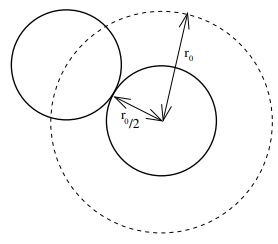
So where does the factor of \(2\) come from? Well, if \(2b\) denotes that physically excluded volume, then if one adds in gas particles one by one, the first can roam in the container’s volume \(V\), the second in \(V-2b\), the third in \(V-4b\), etc. The total \(N\)-dimensional configuration space (NOT phase space!) hypervolume \(\mathcal V\) for \(N\) gas particles is:
\[\mathcal V=\frac{1}{N!}\prod_{n=1}^N(V-2nb)\]
In the limit \(V\ll 2b\), one can check that this hypervolume \(\mathcal V\) reduces to \(\mathcal V=\frac{1}{N!}\left(V-Nb\right)^N\) suggesting that it is indeed \(b\) and not \(2b\) that is the correct correction to the container volume \(V\) in the Van der Waals equation (in other words, \(b\) should be thought of as the excluded configuration space volume contributed by each gas particle).
To summarize, recall the following assumptions that went into the derivation of the Van der Waals equation of state:
- Low density gases \(N/V\ll 1/r_0^3\) (much less dense than the liquid phase!).
- High-temperature \(V_0\ll kT\).
- Hard sphere Pauli repulsion \(V(r)=\infty[r<r_0]\).
So while the Van der Waals equation of state is a significant improvement over the ideal gas law, it too has its limitations.
Universality in Van der Waals Fluids
Recall that taking an ideal gas and turning on Van der Waals interactions described by a long-range attractive Lennard-Jones potential and a short-range repulsive Pauli interaction modifies the equation of state to:
\[p=\frac{NkT}{V-Nb}-a\left(\frac{N}{V}\right)^2\]
One can proceed to plot some isotherms of this van der Waals fluid in the usual \(pV\) state space of the fluid (wiggles are exaggerated):
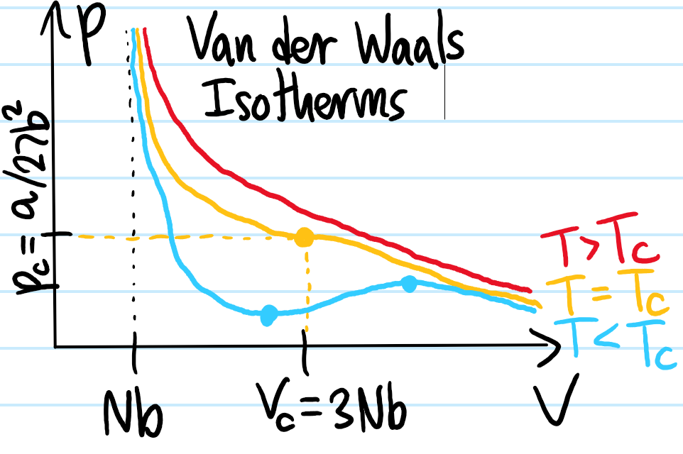
At sufficiently high temperatures \(T>T_c\), the pressure \(p\) decreases monotonically with volume \(V\) along a (roughly) hyperbolic path \(p\propto V^{-1}\) so the Van der Waals fluid is supercritical in this regime (i.e. behaves like a liquid as \(V\to Nb\) and \(p\to\infty\) but otherwise behaves like an ideal gas as \(V\to\infty,p\to 0\)). By contrast, for low temperatures \(T<T_c\), the isotherm is no longer monotonic, experiencing both a local min and a local max. These occur at volumes \(V\) satisfying the cubic equation:
\[\frac{\partial p}{\partial V}=-\frac{NkT}{(V-Nb)^2}+\frac{2aN^2}{V^3}=0\]
It can be checked that the discriminant of the cubic vanishes (corresponding to additionally imposing \(\partial^2p/\partial V^2=0\)) at the critical temperature \(kT_c=8a/27b\), with \(T<T_c\) corresponding to \(3\) real roots and \(T>T_c\) only \(1\) real root (a local max hiding at the unphysical \(V<Nb\) so not shown). The corresponding critical volume \(V_c=3Nb\) and critical pressure \(p_c=a/27b^2\) are easily found and annotated on the figure. In particular, note that the critical compression factor \(Z_c:=p_cV_c/NkT_c\) (not to be confused with the isothermal compressibility \(\kappa_T=-(\partial\ln V/\partial p)_T\) which blows up \(\kappa_T=\infty\) anyways at the critical point) is predicted by the Van der Waals equation to be a universal constant in all Van der Waals fluids:
\[Z_c=\frac{3}{8}=0.375\]
In practice, real fluids have \(Z_c\in\approx[0.2,0.3]\), reflecting the fact that the Van der Waals equation is not so accurate in the liquid regime (because it includes \(2\) fitting parameters \(a,b\) whereas the critical point is defined by \(3\) variables \(p_c,V_c,T_c\), it will always be possible to isolate some kind of universal ratio like this in any equation of state with only \(2\) fit parameters, but not necessarily so for more complicated equations of state). In any case, it definitely outperforms the naive ideal gas prediction \(Z=1\) (i.e. this prediction is just anywhere since there is no notion of criticality in the ideal gas model).
Using the critical variables \(p_c,V_c,T_c\), one can eliminate the fluid-specific constants \(a,b\) from the Van der Waals equation by rewriting it in terms of the reduced pressure \(\hat p:=p/p_c\), the reduced volume \(\hat V:=V/V_c\) and the reduced temperature \(\hat T:=T/T_c\):
\[\hat p=\frac{8\hat T}{3\hat V-1}-\frac{3}{\hat V^2}\]

This universal form of the Van der Waals equation is an instance of the law of corresponding states. Specifically, it is universal in the sense that it’s saying, for all fluids, certain aspects of their physics near their respective critical points look identical. For instance, one has the obvious Taylor expansion \(p-p_c\sim(V-V_c)^3\) as \(V\to V_c\) at the critical point. Two very different fluids will in general have their own very different critical \(p_c\) and \(V_c\), though the Van der Waals equation is making the remarkable claim that if one were to just be handed log-log plots of \(\ln(p-p_c)\) vs. \(\ln(V-V_c)\) for \(p\) close to \(p_c\) and \(V\) close to \(V_c\) in the case of each fluid, then both will have the same slope of \(3\) and differ only by a translation.
Another Van der Waals prediction is the divergence of the isothermal incompressibility \(\kappa_T\sim (T-T_c)^{-1}\) as \(T\to T_c^+\) (this of course agrees with the earlier assertion that exactly at the critical point, \(\kappa_{T=T_c}=\infty\) blows up). Although the Van der Waals equation was historically the first time that this whole theme of “universality at criticality” arose (and which is indeed what is observed experimentally), quantitatively speaking it only produces a rough approximation to the various critical exponents (heuristically this is because fluctuations become more and more important as one approaches the critical point, which is not something that Van der Waals takes into account). For instance, it turns out that actually \(p-p_c\sim(V-V_c)^{\approx 4.2}\) instead, and that \(\kappa_T\sim (T-T_c)^{\approx -1.2}\).
Liquid-To-Gas Phase Transition
Naively, the Van der Waals equation suggests that for a given subcritical isotherm \(\hat T<1\), there are supposedly certain equilibria where the Van der Waals fluid has negative isothermal compressibility \(\kappa_{\hat T}<0\). Such equilibria are obviously unstable. Fortunately, it seems that one can salvage this situation by the fact that
But all points on the \(T<T_C\) isotherm with \(\partial p/\partial V>0\) are unstable equilibria since, if the fluid starts at any such point, then any small perturbation in its volume \(V\) would, according to the isotherm, suggest that it now wants to equilibrate to a higher pressure \(p\), which would push the volume \(V\) even further in the original direction of change, enforcing a positive feedback loop. So instead, only the negative-feedback states with \(\partial p/\partial V<0\) can be observed in practice. For this reason, rather than strictly plotting a \(T<T_C\) Van der Waals isotherm, it would be desirable to replace the unstable section of the isotherm with the actually-experimentally-observed equilibrium states over those range of volumes \(V\).
Although at all temperatures \(T\), each volume \(V\) is associated with some unique equilibrium pressure \(p\), for \(T<T_C\) where monotonicity is broken, there is no longer a bijection between pressures \(p\) and volumes \(V\); in particular, it is clear that for all pressures \(p\) in the blue range highlighted,
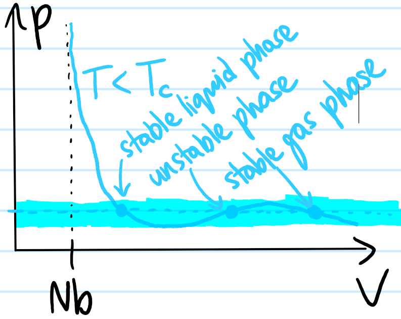
In the case \(T<T_C\), for all pressures \(p\) in the blue range highlighted, the Van der Waals isotherm suggests there are \(3\) equilibrium volumes \(V\) that the system would tend towards if it were not already sitting at one of those volumes (assuming here the volume \(V\) is changeable by e.g. a piston).
Gravity is an anisotropic external input, density filter.
The middle phase is unstable due to its positive gradient \(\partial p/\partial V>0\), however the outer two are stable, and by inspecting not only their corresponding volumes \(V\) but also their isothermal compressibilities \(\kappa_T:=-(\partial\ln V/\partial p)_T\) or equivalently their isothermal bulk moduli \(B_T:=1/\kappa_T\), it is clear that the left point corresponds to a liquid while the right point corresponds to a gas. However, recall that the Van der Waals equation is essentially a second-order virial expansion in the particle density \(N/V\) so although it predicts the existence of a stable liquid phase, any quantitative predictions it makes about such a liquid phase (for which \(N/V\) is not typically small) need to be taken with a grain of salt.
But this begs the question, if the system sits at a pressure \(p\) for which both the liquid and gas phases seem to be stable, what does one actually observe experimentally? The answer is that, in general, there will be a mixture of both the liquid and gas phases. Implicitly here, one is considering the steady state \(t\to\infty\) limit with everything in thermodynamic equilibrium. Mechanical equilibrium is necessarily satisfied because by assumption the pressure \(p\) is fixed on a horizontal line, and thermal equilibrium is also ensured because both phases sit on the same \(T\)-isotherm. The only additional constraint yet to be imposed is diffusive equilibrium, i.e. that the number of particles in each has reached a steady state. This means both the liquid and gas phases, if they were to coexist, would also need to lie at the same chemical potential \(\mu\) (since \(p,T\mu\) are all intensive there is no constraint on the absolute numbers \(N_{\ell},N_g\) of liquid and gas particles, only on their relative proportion \(N_{\ell}/N_g\)). The Maxwell construction shows (proof omitted) that this only happens at a pressure \(p\) for which one has equal areas:
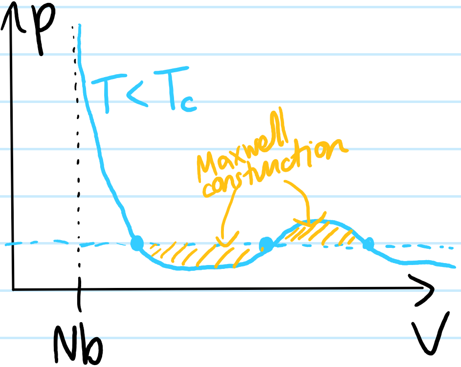
(thus, if the initial pressure \(p\) were not at this specific pressure, then the chemical potentials \(\mu_{\ell}\neq\mu_g\) would initially be unbalanced and particles would begin to diffuse from one phase to the other until the chemical potentials were balanced and the pressure would rise or fall accordingly). Considering the set of temperatures \(T\leq T_C\), for each one it is possible to perform a Maxwell construction to identify exactly which two points on that \(T\)-isotherm lead to equilibrium between the liquid and gas phases, and plot the corresponding \((p_{\ell},V_{\ell}),(p_g,V_g)\); the set of all such pairs in the \(pV\)-plane defines the coexistence curve. This is not to be confused with the spinodal curve which is just the curve passing through the extrema of the Van der Waals isotherms. Sandwiched between these are metastable states.