
Problem #\(1\): What does the phrase “\(N\) coupled harmonic oscillators” mean?
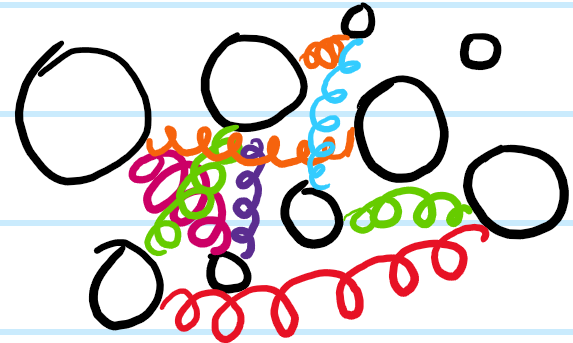
Solution #\(1\): Basically, just think of \(N\) masses \(m_1,m_2,…,m_N\) with some arbitrarily complicated network of springs (each of which could have different spring constants) connecting various pairs of masses together:
Problem #\(2\): Rephrase Solution #\(1\) in more mathematical terms.
Solution #\(2\): The idea is that there are \(N\) degrees of freedom \(x_1,x_2,…,x_N\) and the second time derivative of each one is given by some linear combination of the \(N\) degrees of freedom; packaging into a vector \(\textbf x:=(x_1,x_2,…,x_N)^T\in\textbf R^N\), this means that there exists an \(N\times N\) matrix \(\omega^2\) (independent of \(t\)) such that:
\[\ddot{\textbf x}=-\omega^2\textbf x\]
Problem #\(3\): In general, how does one solve the second-order ODE in Solution #\(2\)?
Solution #\(3\): One way is to first rewrite it as a first-order ODE:
\[\frac{d}{dt}\begin{pmatrix}\textbf x\\\dot{\textbf x}\end{pmatrix}=\begin{pmatrix}0&1\\-\omega_0^2&0\end{pmatrix}\begin{pmatrix}\textbf x\\\dot{\textbf x}\end{pmatrix}\]
from which the solution is immediate:
\[\begin{pmatrix}\textbf x(t)\\\dot{\textbf x}(t)\end{pmatrix}=e^{t\begin{pmatrix}0&1\\-\omega^2&0\end{pmatrix}}\begin{pmatrix}\textbf x(0)\\\dot{\textbf x}(0)\end{pmatrix}\]
and using \(\begin{pmatrix}0&1\\-\omega^2&0\end{pmatrix}^2=-\begin{pmatrix}\omega^2&0\\0&\omega^2\end{pmatrix}\), one has the self-consistent solutions:
\[\textbf x(t)=\cos(\omega t)\textbf x(0)+\omega^{-1}\sin(\omega t)\dot{\textbf x}(0)\]
\[\dot{\textbf x}(t)=-\omega\sin(\omega t)\textbf x(0)+\cos(\omega t)\dot{\textbf x}(0)\]
Problem #\(4\): In practice how would one evaluate the quantities \(\cos(\omega t)\) and \(\omega^{-1}\sin(\omega t)\) appearing in Solution #\(3\)?
Solution #\(4\): One has:
\[\cos(\omega t)=1-\frac{\omega^2 t^2}{2}+\frac{\omega^4t^4}{24}-…\]
\[\omega^{-1}\sin(\omega t)=1-\frac{\omega^2 t^3}{6}+\frac{\omega^4t^5}{120}-…\]
The point is that one needs an efficient way to evaluate powers \(\omega^{2n}\) of the matrix \(\omega^2\) appearing in the equation of motion \(\ddot{\textbf x}=-\omega^2\textbf x\); the standard way to do this is to diagonalize \(\omega^2\).
Problem #\(5\): Interpret the diagonalization of \(\omega^2\) in Solution #\(4\) as a physicist.
Solution #\(5\): Each eigenspace of \(\omega^2\) is called a normal mode of the corresponding system of coupled harmonic oscillators, i.e. a normal mode should be thought of as a pair \((\omega_0,\ker(\omega^2-\omega_0^21))\); since \(\omega^2\) is an \(N\times N\) matrix, there will in general be \(N\) normal modes (assuming \(\omega^2\) is diagonalizable which in practice will always be the case). Viewed in this way, the general dynamics of \(N\) coupled harmonic oscillators consists of a superposition of the \(N\) normal modes of the system, with the coefficients in this superposition determined by the initial conditions \(\textbf x(0),\dot{\textbf x}(0)\).
Physically, because a normal mode is defined by a single eigenfrequency \(\omega_0\), it means that if one were to release the system with exactly the right initial conditions to excite only that one specific normal mode, then all \(N\) coupled harmonic oscillators would oscillate at the same frequency \(\omega_0\) with some relative amplitudes and relative phases between each of their oscillations as encoded in the corresponding eigenspace \(\ker(\omega^2-\omega_0^21)\).
Problem #\(6\): Determine the normal modes of the following systems of coupled harmonic oscillators:
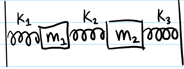
Solution #\(6\): For the \(2\) masses connected to each other and to immoveable walls (equivalent to having infinite masses at those locations):
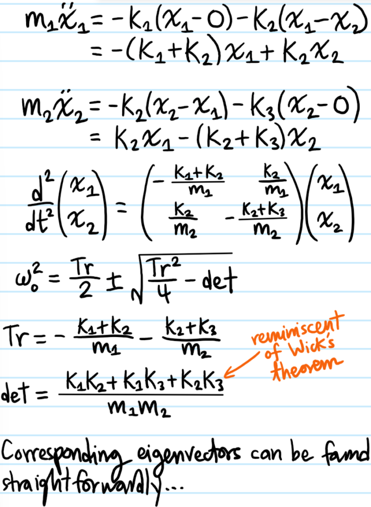
Needless to say for generic \(m_1,m_2,k_1,k_2,k_3\) the normal modes are not so straightforward either. There are of course also many variations of this setup, for instance \(k_3=0\) (i.e. just no wall there) or having \(m_1=m_2\) and \(k_1=k_2=k_3\), etc.
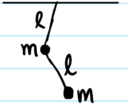
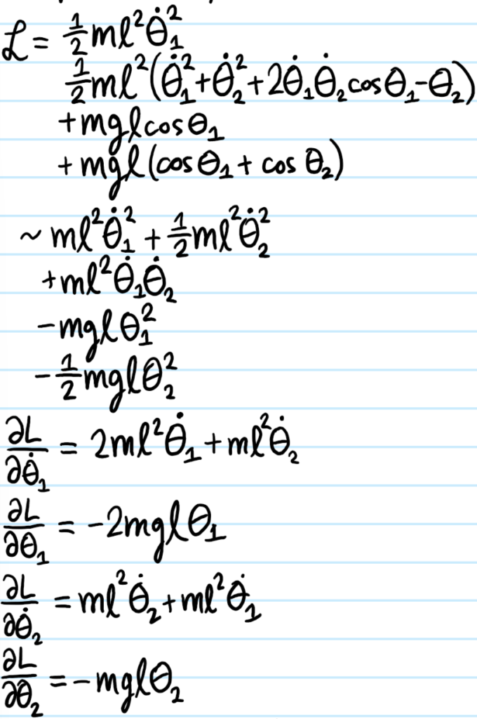
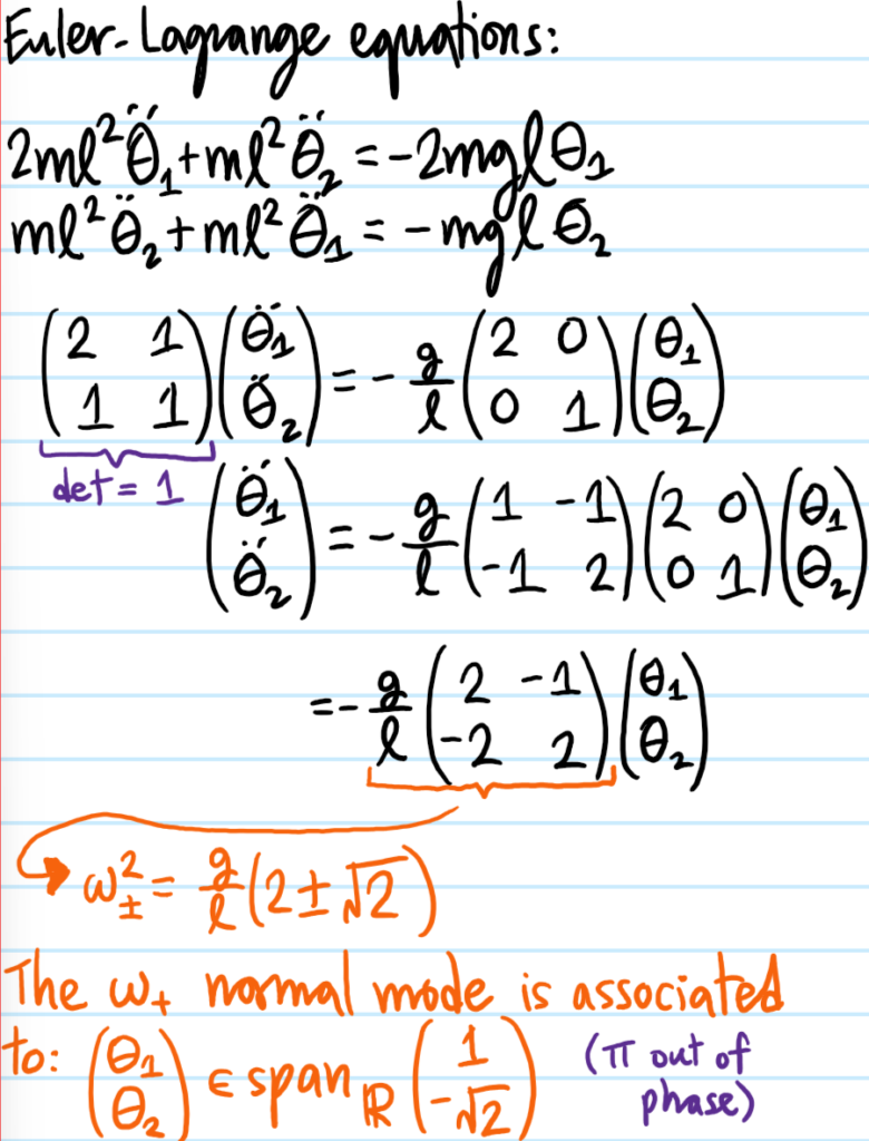
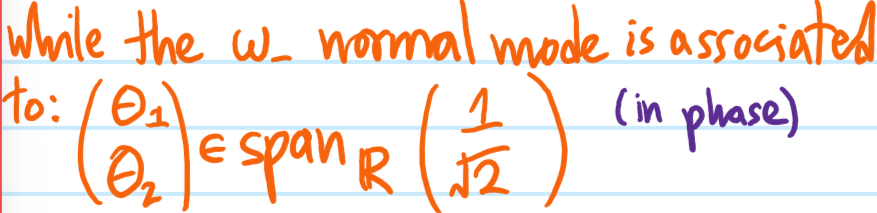
For the double pendulum, it is of course the standard example of a nonlinear dynamical system, but it has a stable fixed point at \(\theta_1=\theta_2=0\) so one can linearize the system about it to obtain \(2\) coupled harmonic oscillators:
Problem #\(7\): Consider extending the first system from Problem #\(6\) from \(N=2\) to \(N\gg 1\) identical masses \(m\) connected by identical springs \(k_s\); in condensed matter physics this is known as the \(1\)D monatomic chain, a classical toy model of a solid. Write down the equation of motion for the displacement \(x_n(t)\) of the \(n\)th atom about its equilibrium where \(2\leq n\leq N-1\); in order for this equation to also be valid for the boundary atoms \(n=1,N\), what (somewhat artificial) assumption does one need to make about the topology of the chain?
Solution #\(7\): For each \(n=2,3,…,N-2,N-1\), the longitudinal displacement satisfies Newton’s second law in the form:
\[m\ddot{x}_n=-k_s(x_n-x_{n-1})-k_s(x_n-x_{n+1})=-k_s(2x_n-x_{n-1}-x_{n+1})\]
If one were to use the same setup as in Problem #\(6\) where the boundary masses are simply connected to walls, or perhaps not connected to anything at all, then this equation of motion would not be valid for \(n=1,N\); however if one imposes an \(S^1\) topology on the chain by identifying \(x_n=x_m\pmod N\) (as if the \(N\) masses had been stringed along a circle instead of a line), then the equation becomes valid for \(n=1,N\) as well. It is for this simple convenient reason that periodic boundary conditions are commonly assumed; for \(N\gg 1\) it is intuitively plausible that the exact choice of boundary conditions shouldn’t affect bulk physics as bulk\(\cap\)boundary\(=\emptyset\).
Problem #\(8\): If \(\Delta x\) denotes the lattice spacing between adjacent masses \(m\) when the entire monatomic chain is at rest, show that the equation of motion coarse grains in the limit \(\Delta x\to 0\) to the \(1\)D free, dispersionless wave equation:
\[\frac{\partial^2\psi}{\partial (ct)^2}-\frac{\partial^2\psi}{\partial x^2}=0\]
where \(c^2=\frac{k_s}{m}(\Delta x)^2\), and the longitudinal displacement \(x_n\mapsto\psi\) has been promoted to a scalar field (and renamed to avoid confusion with the spatial coordinate \(x\)).
Solution #\(8\): One simply has to invoke the symmetric limit formulation of the second derivative:
\[\psi^{\prime\prime}(x)=\lim_{\Delta x\to 0}\frac{\psi(x+\Delta x)+\psi(x-\Delta x)-2\psi(x)}{(\Delta x)^2}\]
Problem #\(9\): Motivated by the result of Solution #\(8\), what is a reasonable ansatz for the longitudinal displacement \(x_n(t)\)? What is the connection between this result and the earlier discussion of normal modes?
Solution #\(9\): Motivated by the usual plane wave solutions \(\psi(x,t)=e^{i(kx-\omega_k t)}\) (with linear dispersion relation \(\omega_k=ck\)) that form the usual Fourier basis for arbitrary solutions to the wave equation, one can similarly write \(x_n(t)=e^{i(kn\Delta x-\omega_k t)}\), where \(x\mapsto n\Delta x\) is the analog of the spatial coordinate. Plugging this into the equation of motion, one finds instead that e.g. a sound wavepacket will disperse as it propagates through this monatomic chain:
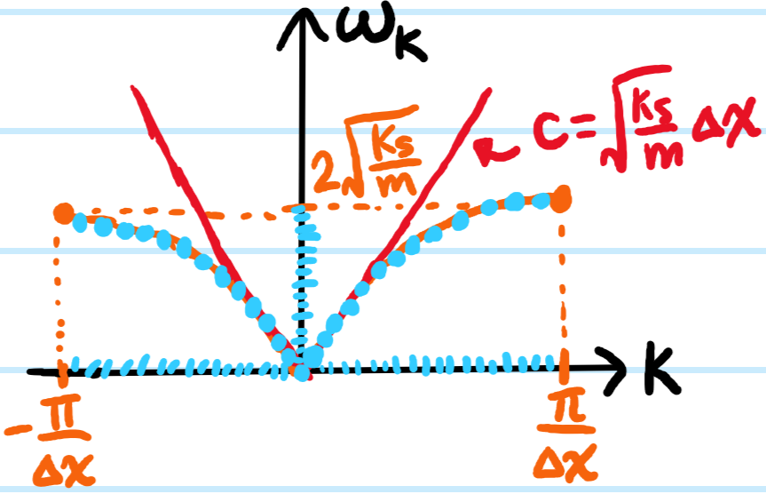
\[\omega_k=2\sqrt{\frac{k_s}{m}}\biggr|\sin\frac{k\Delta x}{2}\biggr|\]
which can be plotted in the first Brillouin zone \(k\Delta x\in[-\pi,\pi)\):
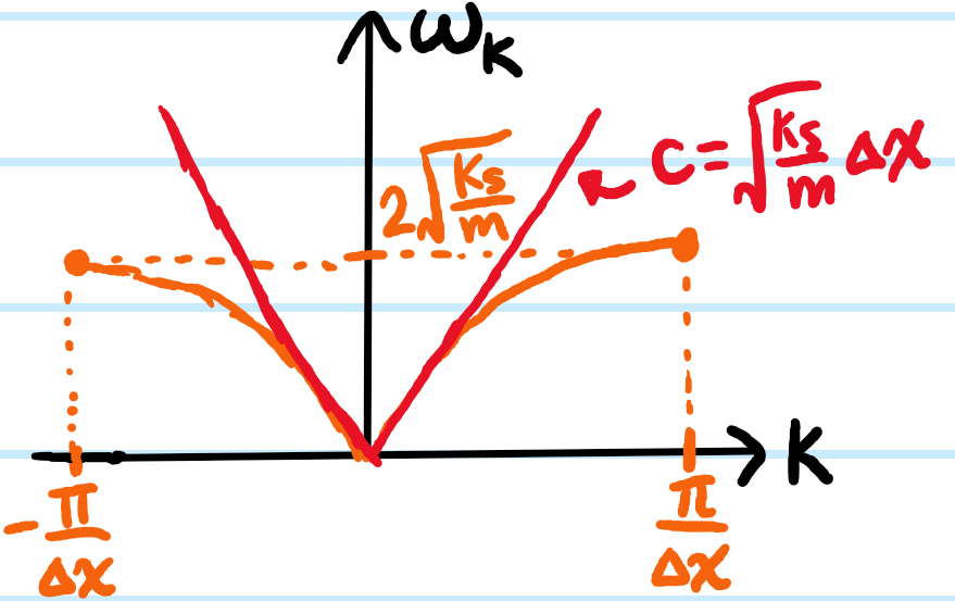
Furthermore, the low-\(|k|\) limit of the group (or in this case phase) velocity \(c=\frac{\partial\omega}{\partial k}\) agrees with the linear dispersion relation from Problem #\(8\); this makes sense because the wave equation was obtained by coarse graining which is equivalent to assuming \(|k|\Delta x\ll 1\).
In general, whenever one finds a linear dispersion relation \(\omega_k\sim k\), it suggests massless particles (e.g. photons, phonons); this is to be contrasted with quadratic dispersion relations \(\omega_k\sim k^2\) which suggest massive particles (e.g. electrons in a tight-binding lattice).
Finally, to connect back to normal modes, because one has \(N\gg 1\) atoms coupled harmonically in the monatomic chain, one of course expects the system to have \(N\gg 1\) normal modes. And indeed the ansatz \(x_n(t)=e^{i(kn\Delta x-\omega_k t)}\) is exactly the form of a normal mode in which all atoms oscillate at the same frequency \(\omega_k\) and (on symmetry grounds) with the same amplitude, but where there is the same constant phase offset of \(x_{n+1}(t)/x_n(t)=e^{ik\Delta x}\) between each pair of adjacent atoms in the chain (again, this phase shift is the same between all pairs of atoms on symmetry grounds). Hopefully this gives the vibe of a sound wave propagating through the chain.
It’s as if we guessed ahead of time the eigenvectors \(x_n(t)\) of the matrix \(\omega^2\) in Solution #\(2\) and then simply acted with \(\omega^2\) on the ansatz eigenvector \( x_n(t)\) and checked that it scales by an eigenvalue \(\omega_k^2\) which gave the dispersion relation (again, usually one finds eigenvalues of a matrix before eigenvectors! This was only possible because of the symmetry; in general, circulant matrices are always diagonalized by the discrete Fourier transform).
Finally, as a minor aside, the earlier choice of periodic boundary condition \(x_{n}(t)\equiv x_{m}(t)\pmod N\) forces \(e^{ikN\Delta x}=1\) which quantizes the wavenumber \(k_m=\frac{2\pi m}{N\Delta x}\) for \(m\in\textbf Z\) (not to be confused with the mass \(m\) obviously); within the first Brillouin zone, there are \(N\) values of \(m=-N/2,…,N/2\) which are the \(N\) normal modes of the chain (i.e. each \(m\to k_m\to\omega_{k_m}\to\omega^2_{k_m}\) corresponding to one of the \(N\) eigenvalues of the \(N\times N\) \(\omega^2\) matrix).
So technically, for a finite monatomic chain of \(N\) atoms, there are only \(N\) combinations of \((k,\omega_k)\) on the dispersion graph which represent permissible normal modes, but as \(N\to\infty\) this quantization will become invisible with \(k,\omega_k\in\textbf R\).
Problem #\(10\): Repeat Problem #\(9\) but for a diatomic chain of masses. Hence show that there are \(2\) qualitatively different classes of normal modes that can be excited in this system, called acoustic modes and optical modes with respective dispersion relations:
\[\omega_{\pm}^2=\frac{k_s}{\mu}\left(1\pm\sqrt{1-\frac{4\mu\sin^2 k\Delta x}{m+M}}\right)\]
with \(k\Delta x\in[-\pi/2,\pi/2)\).
Solution #\(10\): On symmetry grounds, any normal mode would be expected to be of the form:
\[x_{2n}(t):=\alpha e^{i(k2n\Delta x-\omega_k t)}\]
\[x_{2n+1}(t):=\beta e^{i(k(2n+1)\Delta x-\omega_k t)}\]
where \(\alpha,\beta\in\textbf C\). Substituting into the equation of motion, one has:
\[\begin{pmatrix}2k_s-m\omega_k^2&-2k_s\cos k\Delta x\\ -2k_s\cos k\Delta x& 2k_s-M\omega_k^2\end{pmatrix}\begin{pmatrix}\alpha\\\beta\end{pmatrix}=\begin{pmatrix}0\\0\end{pmatrix}\]
in order to get a non-trivial normal mode \((\alpha,\beta)\neq (0,0)\), require the determinant to vanish which gives the desired result (it is instructive to check that the quantity under the square root is indeed non-negative as required by Hermiticity of the matrix).
It is instructive to look at how the diatomic chain reduces to the monatomic chain by setting \(m=M=2\mu\). Then the optical branch becomes:
\[\omega_+=2\sqrt{\frac{k_s}{m}}\biggr|\cos\frac{k\Delta x}{2}\biggr|\]
while the acoustic branch reduces to the single branch that one had earlier for the monatomic chain:
\[\omega_-=2\sqrt{\frac{k_s}{m}}\biggr|\sin\frac{k\Delta x}{2}\biggr|\]
Nevertheless, in a monatomic chain there are no optical phonons, only acoustic phonons because it is \(\Delta x\)-periodic so the Brillouin zone ranges from \(-\pi\leq k\Delta x<\pi\) rather than \(-\pi/2\leq k\Delta x<\pi/2\) as appropriate for a \(2\Delta x\)-periodic diatomic chain (remember, there must still be \(N\) normal modes!). Nevertheless, this does provide intuition for why there is an optical branch (and this procedure is also generalizable to triatomic, etc. chains):
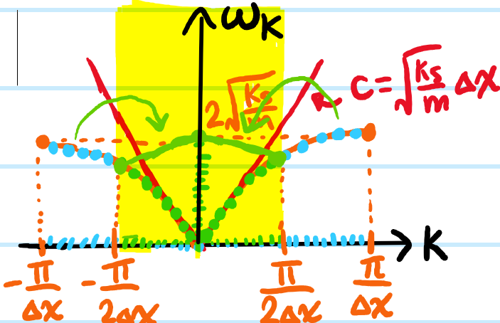
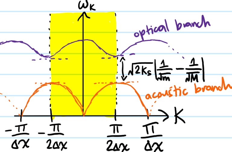
i.e. because the Brillouin zone of the diatomic chain is half as wide as the monatomic chain, so in the reduced Brillouin zone scheme for the diatomic chain, the parts from the monatomic chain are reflected inward, giving the \(\sim\cos\) shape of the optical branch (note these branches are very much analogous to a band structure for phonons instead of electrons; indeed because in a generic diatomic chain \(m\neq M\), this is the origin of the “branch gap” \((\omega_+-\omega_-)_{k=\pm\pi/2\Delta x}=\sqrt{2k_s}|m^{-1/2}-M^{-1/2}|\) between the acoustic and optical branches of the phonon spectrum \(\omega_k\) at the boundary of the Brillouin zone, cf. band gaps. In particular, \((\omega_+-\omega_-)_{k=\pm\pi/2\Delta x}\to 0\) as \(m\to M\)).
Back to the diatomic chain, for \(|k|\Delta x\ll 1\):
\[\omega_+\approx\sqrt{\frac{2k_s}{\mu}}\left(1-\frac{\mu}{2(m+M)}k^2\Delta x^2\right)\to\sqrt{\frac{2k_s}{\mu}}\]
\[\omega_-\approx\sqrt{\frac{2k_s}{m+M}}|k|\Delta x\to 0\]
and the group velocities are:
\[\frac{\partial\omega_{\pm}}{\partial k}=\frac{k_s^2\Delta x\sin 2k\Delta x}{\omega_{\pm}(\mu\omega_{\pm}^2-k_s)(m+M)}\]
and flatten to zero \(\partial\omega_{\pm}/\partial k\to 0\) at the boundary \(k\to\pm\pi/2\Delta x\) of the Brillouin zone, just as one finds in band structure (e.g. for nearly free electrons). All this is summarized in this refined picture:
Problem #\(11\): How do the atoms in the diatomic chain actually move in acoustic vs. optical normal modes?
Solution #\(11\): In general, the phasor ratios of \(m\) vs. \(M\) atom displacements (viewed as functions of \(k\)) are:
\[\left(\frac{\beta}{\alpha}\right)_{\pm}=\left(1-\frac{m\omega_{\pm}^2}{2k_s}\right)\sec k\Delta x\]
There are \(2\) interesting limits of this expression, namely \(k=0\) and \(k=\pm\pi/2\Delta x\). In the former case:
\[\left(\frac{\beta}{\alpha}\right)_{+}(k=0)=-\frac{m}{M}\]
\[\left(\frac{\beta}{\alpha}\right)_{-}(k=0)=1\]
So at low-\(k\), the diatomic chain in an acoustic normal mode looks like neighbouring atoms oscillating in phase with equal amplitude whereas the optical mode looks like a \(\pi\)-radian out-of-phase oscillation with the lighter atoms oscillating more than the heavier atoms by the mass ratio \(M/m\), as intuitively reasonable. This also explains the name “optical branch”; if the atoms in the diatomic chain are in fact ions of opposite charge as in an \(\text{NaCl}\) crystal, then one has pairs of oscillating electric dipoles which can couple to light.
Meanwhile, at the boundary of the Brillouin zone, one finds:
\[\left(\frac{\beta}{\alpha}\right)_{\pm}(k=\pm\pi/2\Delta x)=\frac{M-m\mp|M-m|}{2M}\sec\pm\frac{\pi}{2}\]
where although \(\sec\pm\pi/2=\infty\) diverges, causing \((\beta/\alpha)_-=\infty\), actually the factor in front goes to zero even faster than the secant diverges as \(k\to\pm\pi/2\Delta x\) so that actually \((\beta/\alpha)_+=0\). This is a (longitudinal) standing wave! i.e. in the optical mode, one has nodes at the heavier atoms \(M\) while the light atoms represent displacement antinodes, and vice versa in the acoustic mode (intuitively, \(k=\pi/2\Delta x\Leftrightarrow\lambda=4\Delta x\)).
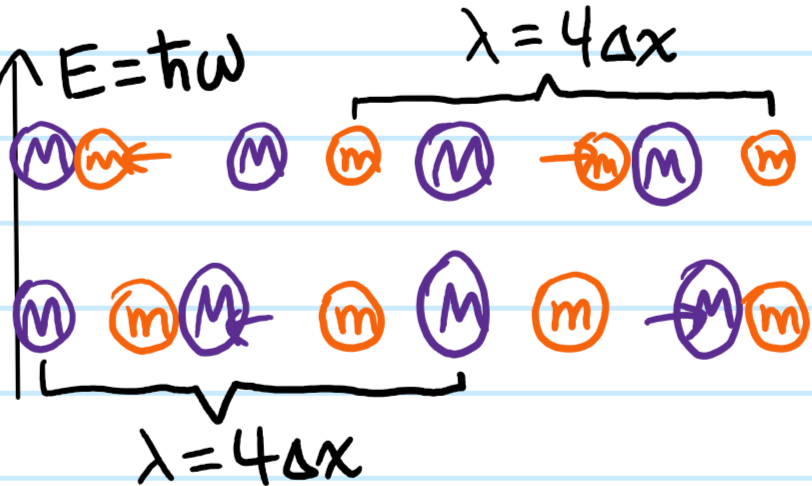
Notice the group velocity \((\partial\omega/\partial k)_{k=\pm\pi/2\Delta x}\) also tends to zero at the Brillouin zone boundary…that’s just another way of saying it’s a standing wave!
Another useful intuition is that, say near \(k=0\), the acoustic and optical normal modes look the way they do such that atoms can be paired up at any moment in time with equal and opposite momenta, giving the overall collective excitation/phonon also zero momentum! So there is a direct connection between \(mv\) momentum and \(\hbar k\) momentum (ACTUALLY ARE WE SURE THIS IS TRUE?).
Problem #\(12\): Just to emphasize again: on the one hand, one can generically refer to \(\omega_k\) as a dispersion relation for a particular kind of wave; here what is a better name for \(\omega_k\)?
Solution #\(12\): The phrase “normal mode spectrum” is useful to keep in mind.