The purpose of this post is to quickly review some fundamentals of classical computation in order to better appreciate the distinctions between classical computing and quantum computing. Note that the word computation itself, whether classical or quantum, basically just means evaluating functions \(f:\alpha^*\to\alpha^*\) defined on the Kleene closure \(\alpha^*\) of an arbitrary alphabet/set \(\alpha\) (recall that sequences of symbols from the alphabet \(\alpha\) are called strings over \(\alpha\) with \(\alpha^*=\bigcup_{n\in\textbf N}\alpha^n\) the set of all strings over \(\alpha\)). However, for any at most countable alphabet \(|\alpha|\in\textbf N\cup\{\aleph_0\}\), the Kleene closure \(\alpha^*\) will be countably infinite \(|\alpha^*|=\aleph_0\), so it should therefore be possible to exhibit a injection \(\alpha^*\to\alpha_{\text{binary}}^*\) from strings in \(\alpha^*\) to bit strings in \(\alpha_{\text{binary}}^*\) where \(\alpha_{\text{binary}}:=\{0,1\}\) is the binary alphabet. In turn, this simply means finding a (binary) encoding \(\mathcal E:\alpha\to\alpha_{\text{binary}}^*\) at the level of the individual symbols in the alphabet \(\alpha\) into bit strings in \(\alpha_{\text{binary}}^*\) and then concatenating together bit strings for individual symbols in \(\alpha\) to obtain bit strings for strings in \(\alpha^*\). In image processing for instance, such an encoding \(\mathcal E\) would be thought of as lossless compression of the data/symbols in the alphabet \(\alpha\), and there are many possible encoding schemes depending on the situation, for instance a fixed-length encoding \(\mathcal E_{\text{FL}}\), or variable-length encodings such as run-length encoding \(\mathcal E_{\text{RL}}\) or Huffman encoding \(\mathcal E_{\text{Huffman}}\). If one uses a fixed-length encoding \(\mathcal E_{\text{FL}}\), then the overhead cost associated with \(\mathcal E_{\text{FL}}\) is linear \(\mathcal E_{\text{FL}}(a_1+a_2)=\mathcal E_{\text{FL}}(a_1)+\mathcal E_{\text{FL}}(a_2)\) for all symbols \(a_1,a_2\in\alpha\) (where here we adapt the Pythonic meaning of \(+\) as a string concatenation; note that the encoding \(\mathcal E_{\text{FL}}\) is technically only defined on the alphabet \(\alpha\), so the statement above is more of a definition of how to extend the domain of \(\mathcal E_{\text{FL}}\) from \(\alpha\) to \(\alpha^*\)). This discussion is just to say that henceforth we can assume without loss of generality that the alphabet \(\alpha=\alpha_{\text{binary}}\) is just the binary alphabet, and so all computations will be concerned with evaluating functions \(f:\{0,1\}^*\to\{0,1\}^*\) which map input bit strings to output bit strings.
Defining a binary language \(\mathcal L\) to be any collection of bit strings \(\mathcal L\subseteq\{0,1\}^*\), the decision problem for \(\mathcal L\) is to compute the indicator function \(\in_{\mathcal L}:\{0,1\}^*\to\{0,1\}^*\) of \(\mathcal L\) defined for all input bit strings \(\xi\in\{0,1\}^*\) by the Iverson bracket \(\in_{\mathcal L}(\xi):=[\xi\in\mathcal L]\). Note however that although in general we allow the codomain \(\{0,1\}^*\) of the function \(\in_{\mathcal L}\) being computed to consist of output bit strings of arbitrary length, in fact for binary language decision problems the range \(\in_{\mathcal L}(\{0,1\}^*)\) as manifest in the Iverson bracket is restricted to the \(2\) possible one-bit strings \(\in_{\mathcal L}(\{0,1\}^*)=\{0,1\}\subseteq\{0,1\}^*\). A very important example of a decision problem is primality testing where the binary language \(\mathcal L:=\{10,11,101,111,1011,…\}\) consists of all the prime numbers. The decision problem of primality testing is a decidable decision problem by virtue of e.g. the AKS primality test. On the contrary, there unfortunately do also exist undecidable decision problems, examples being the halting problem, Hilbert’s tenth problem, etc. The notion of decidability is specific to decision problems and generalizes to non-decision problems via the notion of computability.
Circuit Model of Classical Computation
Recall that a computation is an evaluation of a function \(f:\{0,1\}^*\to\{0,1\}^*\). A computational model \(\mathcal M\) is any collection \(\mathcal M=\{\Gamma_i:\{0,1\}^*\to\{0,1\}^*|\Gamma_i(\xi)\in O_{|\xi|\to\infty}(1)\}\) of computational steps \(\Gamma_i\in\mathcal M\) considered legal within the framework of \(\mathcal M\), and any well-defined sequence \(\Gamma_1\circ\Gamma_2\circ\Gamma_3…=f\) of such computational steps that compose to the function \(f\) of interest is called an algorithm for computing \(f\) in \(\mathcal M\). Historically, many computational models \(\mathcal M\) (e.g. Turing machines, general recursive functions, lambda calculus, Post machines, register machines) have been proposed in which the nature of the allowed computational steps \(\Gamma_i\in\mathcal M\) seem a priori to give rise to different classes of computable functions \(f\) (i.e. functions \(f\) for which there even exists \(\exists\) some algorithm \(\Gamma_1\circ\Gamma_2\circ\Gamma_3…=f\) for computing \(f\)). However, the Church-Turing thesis is an informal conjecture/axiom in computability theory which roughly asserts that any “reasonable” computational model \(\mathcal M\) one can dream up will in fact have neither greater nor less computing power compared with any other “reasonable” computational model \(\mathcal M’\cong\mathcal M\). Thus, for the purposes of a smoother transition from classical computing to quantum computing, we will henceforth take the circuit model \(\mathcal M_{\text{circuit}}\) to be our computational model. In the circuit model of classical computation \(\mathcal M_{\text{circuit}}\), the allowed computational steps are the \(3\) logic gates \(\mathcal M_{\text{circuit}}=\{\text{AND},\text{OR},\text{NOT}\}\) which form a universal set for arbitrary logic circuits/Boolean functions (though the \(\text{OR}\) gate is actually redundant! see here). For instance, binary adder/multiplier logic circuits are not considered to be computational steps in the circuit model \(\mathcal M_{\text{circuit}}\) because say for two input bit strings \(\xi_1,\xi_2\) of the same length \(n=|\xi_1|=|\xi_2|\) they are not \(O_{n\to\infty}(1)\) as required.
Randomized Classical Computational Models
In anticipation of the randomness inherent in outputs of quantum computations, it will be helpful to quickly review what it means for a classical computational model (such as the circuit model of classical computation) to be randomized. This means that when computing a function \(f:\{0,1\}^*\to\{0,1\}^*\), any input bit string \(\xi\in\{0,1\}^*\) is also concatenated \(\xi\mapsto \xi+\xi_{\text{random}}\) with a uniformly random input bit string from a hypothetical random number generator such as \(\xi_{\text{random}}=011011010001001\in\{0,1\}^*\) (so for each run of the computation, even for the same input bit string \(\xi\), the input bit string \(\xi_{\text{random}}\) will probably be different from the previous run and thus the output bit string of the computation will be a sample from a probability distribution) but otherwise one now just chugs the total input bit string \(\xi+\xi_{\text{random}}\) through some sequence of computational steps \(\Gamma_1,\Gamma_2,…\) within that computational model. For instance, in the circuit model, if one desires a particular logic gate \(\Gamma\) in a computation to act with \(50\%\) probability as an \(\text{AND}\) gate and with \(50\%\) probability as an \(\text{OR}\) gate, then one can define \(\Gamma:\{0,1\}^3\to\{0,1\}\) to take an input bit string \(b_1b_2b_3\) of length \(3\) (i.e. \(3\) input bits) but where say the third input bit \(b_3\) is one of the random input bits in the string \(\xi_{\text{random}}\) and determines the nature of the logic gate \(\Gamma\) according to:
\[\Gamma(b_1,b_2,b_3):=\begin{cases}
\text{AND}(b_1,b_2) & \text{if } b_3 = 0 \\
\text{OR}(b_1,b_2) & \text{if } b_3 = 1
\end{cases}\]
Among randomized computational models, there are \(2\) subclasses: Las Vegas algorithms such as the quicksort algorithm which emphasize correctness of the computational output bit string and Monte Carlo “algorithms” such as Miller-Rabin primality testing which emphasize high probability of correctness of the computational output bit string.
Finally, a note about determinism in computational models. Classical computational models are always deterministic because \(f\) is a function. I would argue that even randomized classical computational models are deterministic because, if for two runs the exact same random bit string \(\xi_{\text{random}}\) happens to be inputted, then the output bit string \(f(\xi+\xi_{\text{random}})\in\{0,1\}^*\) must deterministically be the same. So what would be a non-deterministic computational model? Basically, the God-like magical power of being able to just instantaneously “guess” the correct output bit string \(f(\xi)\in\{0,1\}^*\) for any input bit string \(\xi\in\{0,1\}^*\). Such a non-deterministic computer cannot exist, but is an important theoretical construct for defining the nondeterministic polynomial time complexity class \(NP\) which will be elaborated in the following section.
Classical Complexity Classes
If, in some computational model \(\mathcal M\), someone has found an algorithm \(\Gamma_1\circ\Gamma_2\circ\Gamma_3…=f\) for computing \(f\) (hopefully correctly or at least with high probability of being correct such as in Monte Carlo “algorithms”), then one can always ask about how efficient the algorithm \(\Gamma_1\circ\Gamma_2\circ\Gamma_3…\) is at computing \(f\). This is, in computer science lingo, a question of the algorithm’s complexity. Associated to any algorithm \(\Gamma_1\circ\Gamma_2\circ\Gamma_3…\) are \(2\) distinct kinds of complexity: time complexity (i.e. the number of computational steps \(\Gamma_i\) in the algorithm sequence \(\Gamma_1\circ\Gamma_2\circ\Gamma_3…\)) and space complexity (i.e. “amount” of memory/”RAM” used during execution of the algorithm sequence \(\Gamma_1\circ\Gamma_2\circ\Gamma_3…\)). In general, both the time complexity and space complexity of an algorithm \(\Gamma_1\circ\Gamma_2\circ\Gamma_3…\) are to be viewed as functions of which particular input bit string \(\xi\in\{0,1\}^*\) is fed into the algorithm \(\xi\mapsto\Gamma_1\circ\Gamma_2\circ\Gamma_3…(\xi)\) where in general, input bit strings \(\xi\in\{0,1\}^*\) of longer length \(|\xi|\) may be expected to require greater time complexity \(T(\xi)\) and space complexity \(Sp(\xi)\). More precisely, one is often interested in the behavior of the worst-case time complexity \(T^*(n):=\sup_{\xi\in\{0,1\}^n}T(\xi)\) of the algorithm \(\Gamma_1\circ\Gamma_2\circ\Gamma_3…\) in the asymptotic \(n\to\infty\) limit of longer and longer input bit strings \(\xi\in\{0,1\}^*\) and likewise the behavior of the worst-case space complexity \(Sp^*(n):=\sup_{\xi\in\{0,1\}^n}Sp(\xi)\) in the asymptotic \(n\to\infty\) limit. Sometimes though it’s also interesting to analyze the algorithm’s average time complexity \(\bar T(n):=\frac{1}{2^n}\sum_{\xi\in\{0,1\}^n}T(\xi)\) or the average space complexity \(\bar{Sp}(n):=\frac{1}{2^n}\sum_{\xi\in\{0,1\}^n}Sp(\xi)\), both asymptotically \(n\to\infty\).
Example: For a list of length \(n\in\textbf N\), the linear search algorithm has (both worst-case and average) time complexity that scales asymptotically as \(T^*_{\text{linear search}}(n),\bar T_{\text{linear search}}(n)\in O_{n\to\infty}(n)\) but (both worst-case and average) space complexity that scales asymptotically as \(Sp^*_{\text{linear search}}(n),\bar{Sp}_{\text{linear search}}(n)\in O_{n\to\infty}(1)\). By contrast, the merge sort algorithm has (both worst-case and average) time complexity that scales asymptotically as \(T^*_{\text{merge sort}}(n),\bar T_{\text{merge sort}}(n)\in O_{n\to\infty}(n\log n)\) and (both worst-case and average) space complexity that scales asymptotically as \(Sp^*_{\text{merge sort}}(n),\bar{Sp}_{\text{merge sort}}(n)\in O_{n\to\infty}(n)\). This is obvious, but note that searching a list vs. sorting a list are different computations so one cannot just directly compare these algorithm’s asymptotic spacetime complexities to declare linear search is “more efficient” than merge sort; however binary search is indeed an asymptotically more efficient search algorithm than linear search as measured by their spacetime complexities in the worst-case or averaged senses.
Recall that a decision problem concerns the computation of the indicator function \(\in_{\mathcal L}:\{0,1\}^*\to\{0,1\}\) of a binary language \(\mathcal L\subseteq\{0,1\}^*\) of bit strings. To this effect, we define:
Definition (\(\textbf P\)): The polynomial time complexity class \(\textbf P\) is defined to be the set of all binary languages \(\mathcal L\), or equivalently decision problems, for which there exists an algorithm \(\Gamma_1\circ\Gamma_2\circ\Gamma_3…=\in_{\mathcal L}\) that computes the indicator function \(\in_{\mathcal L}:\{0,1\}^*\to\{0,1\}\) with worst-case time complexity \(T^*_{\Gamma_1\circ\Gamma_2\circ\Gamma_3…}(n)\in\bigcup_{p\in\textbf N}O_{n\to\infty}(n^p)\).
Notice in the definition that we haven’t specified a computational model \(\mathcal M\) from which we derive the computational steps \(\Gamma_i\in\mathcal M\). Indeed, it turns out that the polynomial time complexity class \(\textbf P\) (as with all other complexity classes) is robust with respect to whichever computational model \(\mathcal M\) one chooses to use in the sense that a given binary language/decision problem is in \(\textbf P\) in one computational model \(\mathcal M\) if and only if it’s in \(\textbf P\) in any other Church-Turing equivalent computational model \(\mathcal M’\). Also, note that the polynomial time complexity class \(\textbf P\) doesn’t a priori impose any constraints on the (worst-case or average) space complexity \(Sp_{\Gamma_1\circ\Gamma_2\circ\Gamma_3…}(n)\) of the algorithm. Nonetheless, one can show that \(\textbf P\subseteq \textbf{PSPACE}\) where \(\textbf{PSPACE}\) is the polynomial space complexity class defined verbatim to the polynomial time complexity class \(\textbf P\) except replacing the word “time” with “space” and thus \(T\mapsto Sp\). Whether or not the reverse inclusion \(\textbf{PSPACE}\subseteq \textbf{P}\) is true is still an open question!
Examples: Primality testing is a decision problem which recently (thanks to the AKS primality test) has been shown to be in the polynomial time complexity class \(\textbf P\) (and therefore also in \(\textbf{PSPACE}\)). Note that a naive primality test in which we take a given \(N\in\textbf Z^+\) and divide it by each positive integer \(\leq\sqrt{N}\) does not constitute a polynomial-time algorithm for primality testing. This is because \(\sqrt{N}=2^{\log_2(N)/2}\), but \(n:=\log_2(N)\) is the actual length of the input bit string for \(N\) so therefore we see that this naive primality test algorithm \(T^*_{\text{naive primality test}}(n)\in O_{n\to\infty}(2^n)\) is actually exponential-time. Although it may seem that list searching/ sorting problems are also members of the polynomial time complexity class \(\textbf P\) (thanks to e.g. linear search, binary search, merge sort, etc.), this is strictly speaking only the case if one reframes the original search/sorting problem into a decision problem like “does this list contain the bit string \(1011\)” so that the binary language \(\mathcal L=\{1011\}\) is singleton. Otherwise, one would more accurately consider list searching/sorting problems to be in the complexity class \(\textbf{FP}\) of “functions”.
Owing to the existence of randomized computation leading to randomized algorithms (in particular Monte Carlo algorithms), we also have:
Definition (\(\textbf{BPP}\)): The bounded error probabilistic polynomial time complexity class \(\textbf{BPP}\) is defined to be the set of all binary languages \(\mathcal L\), or equivalently decision problems, for which there exists a randomized algorithm \(\Gamma_1\circ\Gamma_2\circ\Gamma_3…\approx \in_{\mathcal L}\) that attempts to compute the indicator function \(\in_{\mathcal L}:\{0,1\}^*\to\{0,1\}\) with worst-case time complexity \(T^*_{\Gamma_1\circ\Gamma_2\circ\Gamma_3…}(n)\in\bigcup_{q\in\textbf N}O_{n\to\infty}(n^q)\) and correctness probability \(p(\xi)\in(1/2,1]\) for all input bit strings \(\xi\in\{0,1\}^*\) (commonly just declared to be \(\geq 2/3\), though this is arbitrary because one can consider a new algorithm defined by running arbitrarily many Bernoulli trials of the original algorithm, taking the majority decision, and applying the Chernoff bound; thus it suffices to find a Monte Carlo algorithm with \(p(\xi)\in(1/2,1)\) or a Las Vegas algorithm with \(p(\xi)=1\)).
According to Cobham’s thesis, the bounded error probabilistic polynomial time complexity class \(\textbf{BPP}\) (with \(\textbf P\subseteq\textbf{BPP}\) obviously contained therein) of decision problems are considered “classically feasible decision problems” and so the goal of computer scientists is to prove that various \(\mathcal L\)-decision problems are in \(\textbf{BPP}\) by devising clever (possibly randomized) polynomial-time algorithms to compute their corresponding indicator functions (either always correctly or more often than not correctly!). Decision problems which are not in \(\textbf{BPP}\) (or more precisely, haven’t been shown to be in \(\textbf{BPP}\) because no one has discovered a polynomial-time algorithm to compute their indicator functions yet) are therefore the hardest decision problems to solve. Among these are:
Definition (\(\textbf{NP}\)): The nondeterministic polynomial time complexity class \(\textbf{NP}\) is defined to be the set of all binary languages \(\mathcal L\), or equivalently decision problems, for which there exists a nondeterministic algorithm \(\Gamma_{\text{God}}=\in_{\mathcal L}\) that computes the indicator function \(\in_{\mathcal L}:\{0,1\}^*\to\{0,1\}\) with worst-case time complexity \(T^*_{\Gamma_{\text{God}}}(n)\in\bigcup_{p\in\textbf N}O_{n\to\infty}(n^p)\).
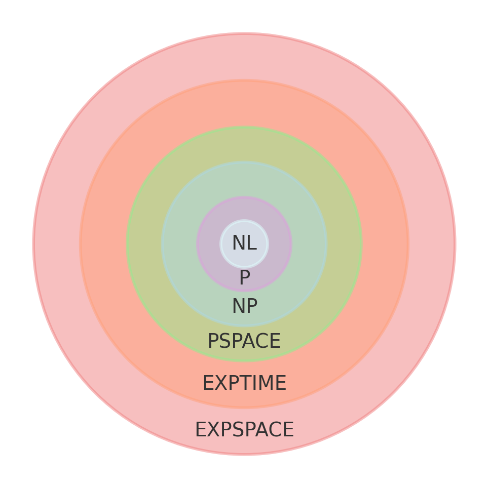
In other words, an \(\mathcal L\)-decision problem is in \(\mathcal L\in\textbf{NP}\) iff its corresponding \(\mathcal L\)-verification decision problem concerning the computation of the function \([\xi\in]\) is in \(\textbf P\). The following diagram summarizes the current state of knowledge as of \(2024\), October \(3\)rd (note that the relationship between \(\textbf{BPP}\) and \(\textbf{NP}\) is still not known!):