
Problem: Explain how a hard-margin support vector machine would perform binary classification.
Solution: Conceptually, it’s simple. Given a training set of \(N\) feature vectors \(\mathbf x_1,…,\mathbf x_N\in\mathbf R^n\) each associated with some binary target label \(y_1,…,y_N\in\{-1,1\}\) (notice the \(2\) binary classes are \(y=-1\) and \(y=1\) rather than the more conventional \(y=0\) and \(y=1\); this is simply a matter of convenience), the goal of an SVM is to compute the unique hyperplane in \(\mathbf R^n\) that will separate the \(y=-1\) and \(y=1\) classes as “best” as possible. For \(n=2\) this can be visualized as trying to find the “widest possible street” between \(2\) neighborhoods:
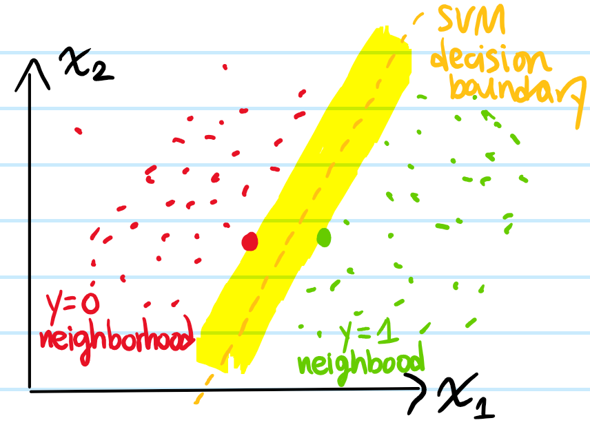
Mathematically, if the hyperplane decision boundary \(\mathbf w\cdot\mathbf x+b=0\) is defined by a normal vector \(\mathbf w\in\mathbf R^n\) such that the SVM classifies points with \(\mathbf w\cdot\mathbf x+b\geq 0\) as \(y=1\) and \(\mathbf w\cdot\mathbf x+b\leq 0\) as \(y=-1\) (more compactly, \(\hat y_{\text{SVM}}(\mathbf x|\mathbf w,b)=\text{sgn}(\mathbf w\cdot\mathbf x+b)\)), and the overall normalization of \(\mathbf w\) and \(b\) is fixed by stipulating that the “gutters” of the street are defined by the hyperplanes \(\mathbf w\cdot\mathbf x+b=\pm 1\) passing through the support (feature) vectors (drawn as bigger red/green dots in the diagram), then the “width of the street” is the distance between these \(2\) “gutter hyperplanes”, namely \(2/|\mathbf w|\). Since one would like to maximize this margin \(2/|\mathbf w|\), this is equivalent to minimizing the quadratic \(|\mathbf w|^2/2\). Thus, one can formulate this “hard-margin SVM” algorithm as the programming problem:
\[\text{argmin}_{\mathbf w\in\mathbf R^n,b\in\mathbf R:\forall i=1,…,N,y_i(\mathbf w\cdot\mathbf x_i+b)\geq 1}\frac{|\mathbf w|^2}{2}\]
where the \(N\) constraints \(y_i(\mathbf w\cdot\mathbf x_i+b)\geq 1\) (or vectorially \(\mathbf y\odot(X^T\mathbf w+b\mathbf{1})\geq\mathbf 1\)) are just saying that all \(N\) feature vectors \(\mathbf x_1,…,\mathbf x_N\) in the training set should lie on the correct side of the decision boundary hyperplane \(\mathbf w\cdot\mathbf x+b=0\).
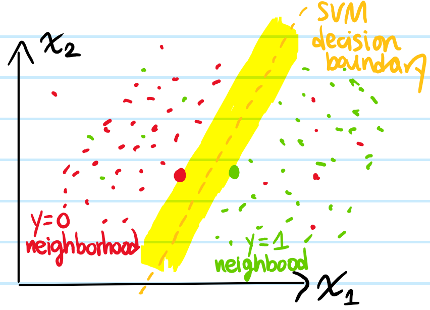
Problem: What is the glaring problem with a hard-margin SVM? How does a soft-margin SVM help to address this issue?
Solution: The basic problem is that the hard-margin SVM is way too sensitive to outliers, e.g. a single \(y=-1\) feature vector amidst the \(y=1\) neighborhood would cause the hard-margin SVM to be unable to find a solution (because indeed there would be no hyperplane that perfectly separates all the training data into their correct classes). Intuitively, it seems like in such a case the best way to deal with this bias-variance tradeoff is to shrug and ignore the outliers:
Mathematically, the usual way to encode this is by introducing \(N\) “slack variables” \(\xi_1,…,\xi_N\geq 0\) such that the earlier \(N\) constraints are relaxed to \(y_i(\mathbf w\cdot\mathbf x_i+b)\geq 1-\xi_i\). However, to avoid cutting too much slack (i.e. incurring too much misclassification on the training set), their use should be penalized by the \(\ell^1\)-norm \(|\boldsymbol{\xi}|_1:=\boldsymbol{\xi}\cdot\mathbf{1}=\sum_{i=1}^N\xi_i\). To this effect, the programming problem is modified to that of soft-margin SVM:
\[\text{argmin}_{\mathbf w\in\mathbf R^n,b\in\mathbf R,\boldsymbol{\xi}\in\mathbf R^N:\mathbf y\odot(X^T\mathbf w+b\mathbf{1})\geq\mathbf 1-\boldsymbol{\xi},\boldsymbol{\xi}\geq\mathbf 0}\frac{|\mathbf w|^2}{2}+C|\boldsymbol{\xi}|_1\]
where \(C\geq 0\) is a “strictness” hyperparameter that must be selected ahead of time to balance hard vs. soft SVM.
Problem: The above represents the primal formulation of the programming problem in terms of so-called primal variables \(\mathbf w,b,\boldsymbol{\xi}\). Show how the KKT conditions enable one to obtain a corresponding dual formulation of the programming problem in terms of a dual variable \(\boldsymbol{\lambda}\):
\[\text{argmax}_{\boldsymbol{\lambda}\in\mathbf R^N:\boldsymbol{\lambda}\cdot\mathbf y=0,\mathbf 0\leq\boldsymbol{\lambda}\leq C\mathbf 1}|\boldsymbol{\lambda}|_1-\frac{1}{2}(\boldsymbol{\lambda}\odot\mathbf y)X^TX(\boldsymbol{\lambda}\odot\mathbf y)\]
Solution: The idea is to combine the \(2\) constraints \(\mathbf y\odot(X^T\mathbf w+b\mathbf{1})\geq\mathbf 1-\boldsymbol{\xi}\) and \(\boldsymbol{\xi}\geq\mathbf 0\) using \(2\) KKT multipliers \(\boldsymbol{\lambda},\boldsymbol{\mu}\) into the Lagrangian:
\[L(\mathbf w,b,\boldsymbol{\xi},\boldsymbol{\lambda},\boldsymbol{\mu})=\frac{|\mathbf w|^2}{2}+C|\boldsymbol{\xi}|_1-\boldsymbol{\lambda}\cdot(\mathbf y\odot(X^T\mathbf w+b\mathbf{1})-\mathbf 1+\boldsymbol{\xi})-\boldsymbol{\mu}\cdot\boldsymbol{\xi}\]
The KKT necessary conditions assert:
\[\frac{\partial L}{\partial\mathbf w}=\mathbf 0\Rightarrow\mathbf w=X(\boldsymbol{\lambda}\odot\mathbf y)\]
\[\frac{\partial L}{\partial b}=0\Rightarrow\boldsymbol{\lambda}\cdot\mathbf y=0\]
\[\frac{\partial L}{\partial\boldsymbol{\xi}}=\mathbf 0\Rightarrow C\mathbf 1=\boldsymbol{\lambda}+\boldsymbol{\mu}\]
in addition to the \(2\) original constraints on the primal variables (primal feasibility), and dual feasibility \(\boldsymbol{\lambda},\boldsymbol{\mu}\geq\mathbf 0\) on both dual variables (as a corollary, \(\mathbf 0\leq\boldsymbol{\lambda}\leq C\mathbf 1\)), and complementary slackness \(\boldsymbol{\lambda}\odot(\mathbf y\odot(X^T\mathbf w+b\mathbf{1})-\mathbf 1+\boldsymbol{\xi})=\boldsymbol{\mu}\odot\boldsymbol{\xi}=\mathbf 0\). The idea of the support vectors is clearly seen in the \(1^{\text{st}}\) of these complementary slackness conditions.
By substituting the stationary conditions found back into the Lagrangian, one can eliminate all the primal variables (and even eliminate one of the dual variables \(\boldsymbol{\mu}\)) to obtain the claim:
\[L(\boldsymbol{\lambda})=|\boldsymbol{\lambda}|_1-\frac{1}{2}(\boldsymbol{\lambda}\odot\mathbf y)X^TX(\boldsymbol{\lambda}\odot\mathbf y)\]
which is a standard quadratic programming exercise with efficient solutions for \(\boldsymbol{\lambda}\).
(mention something about strong duality as enabling a min-max interchange of primal vs. dual?)
Problem: Although soft-margin SVM is a significant improvement over hard-margin SVM, it too has a glaring issue. What is that issue and how can it be addressed?
Solution: Whether hard-margin or soft-margin, SVMs are ultimately linear binary classifiers; they can only directly learn a hyperplane decision boundary. Therefore, if the data is simply linearly inseparable, then even soft-margin SVM would be unwise to apply directly.
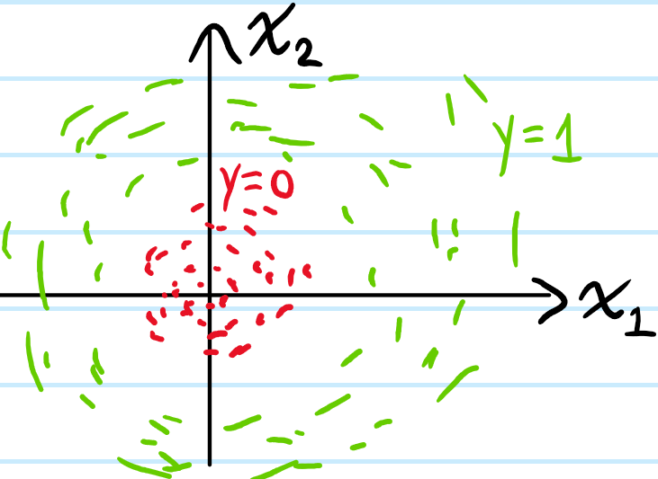
However, there is a creative solution; just take the \(N\) feature vectors \(\mathbf x_1,…,\mathbf x_N\in\mathbf R^n\) and apply a nonlinear transformation \(\prime:\mathbf R^n\to\mathbf R^{>n}\) from the current feature space \(\mathbf R^n\) to some higher-dimensional feature space \(\mathbf R^{>n}\) (essentially a kind of feature engineering), thereby obtaining \(N\) transformed feature vectors \(\mathbf x’_1,…,\mathbf x’_N\in\mathbf R^{>n}\). Ideally, if the nonlinear transformation \(\prime\) is well-chosen, then the transformed feature vectors \(\mathbf x’_1,…,\mathbf x’_N\) will become linearly separable in the higher-dimensional feature space \(\mathbf R^{>n}\), in which case the usual soft-margin SVM may be applied in \(\mathbf R^{>n}\). Then, applying the inverse nonlinear mapping \(\prime^{-1}:\mathbf R^{>n}\to\mathbf R^n\) back to the original feature space \(\mathbf R^n\), the SVM (soft) maximal-margin hyperplane in \(\mathbf R^{>n}\) would be transformed into some nonlinear decision boundary back in \(\mathbf R^n\), thereby effectively extending the applicability of the SVM method to linearly inseparable data! See this YouTube video for an example.
Problem: Continuing off the previous problem, suppose one is already in the transformed space with feature vectors \(\mathbf x’_1,…,\mathbf x’_N\in\mathbf R^{>n}\), and one has solved the dual programming problem in this space to obtain some optimal \(\boldsymbol{\lambda}\in\mathbf R^N\). How is binary classification thus performed?
Solution: Based on the previous analysis, the SVM binary classifier in this transformed feature space \(\mathbf R^{>n}\) may be written:
\[\hat y_{\text{SVM}}(\mathbf x’)=\text{sgn}(\mathbf w\cdot\mathbf x’+b)=\text{sgn}\left(\sum_{i=1}^N\lambda_iy_i\mathbf x’\cdot\mathbf x’_i+y_S-\sum_{i=1}^N\lambda_iy_i\mathbf x’_S\cdot\mathbf x’_i\right)\]
where \(\mathbf x’_S\) is any support feature vector. Note by complementary slackness that most \(\lambda_i=0\) are vanishing (corresponding non-support feature vectors \(\mathbf x_i\)), so the sums \(\sum_{i=1}^N\) may also be written as sums over only support vectors.
Problem: Explain how the expression above can be simplified by means of the kernel trick.
Solution: Basically, the feature space transformation \(\prime:\mathbf R^n\to\mathbf R^{>n}\) is a complicated mapping of vectors to vectors. By contrast, only their scalar dot products \(\mathbf x’\cdot\mathbf x’_i\) appear in the SVM classifier \(\hat y_{\text{SVM}}(\mathbf x)\), and scalars are simpler than vectors. The kernel trick essentially invites one to forget about the details of the transformation \(\prime\) and just directly specify an analytical expression for the dot product in the transformed feature space \(K(\mathbf x,\tilde{\mathbf x}):=\mathbf x’\cdot\tilde{\mathbf x}’\), where here \(K:\mathbf R^n\times\mathbf R^n\to\mathbf R\) is called the kernel function. Effectively, this means one never has to actually visit the transformed feature space \(\mathbf R^{>n}\) since the kernel is perfectly happy to just take the feature vectors in the original space \(\mathbf R^n\). Thus, one can write:
\[\hat y_{\text{SVM}}(\mathbf x)=\text{sgn}(\mathbf w\cdot\mathbf x’+b)=\text{sgn}\left(\sum_{i=1}^N\lambda_iy_iK(\mathbf x,\mathbf x_i)+y_S-\sum_{i=1}^N\lambda_iy_iK(\mathbf x_S,\mathbf x_i)\right)\]
Problem: What is the Gaussian (radial basis function) kernel \(K_{\sigma}(\mathbf x,\tilde{\mathbf x})\)? Sketch why it’s a valid kernel function.
Solution: This is by far the most popular kernel for nonlinear SVM classification, involving a hyperparameter \(\sigma\):
\[K_{\sigma}(\mathbf x,\tilde{\mathbf x})=e^{-|\mathbf x-\tilde{\mathbf x}|^2/2\sigma^2}\]
algebraically, it is clearly equivalent to:
\[K_{\sigma}(\mathbf x,\tilde{\mathbf x})=e^{-|\mathbf x|^2/2\sigma^2}e^{-|\tilde{\mathbf x}|^2/2\sigma^2}e^{\mathbf x\cdot\tilde{\mathbf x}/\sigma^2}\]
Taylor expanding the last factor:
\[K_{\sigma}(\mathbf x,\tilde{\mathbf x})=e^{-|\mathbf x|^2/2\sigma^2}e^{-|\tilde{\mathbf x}|^2/2\sigma^2}\sum_{d=0}^{\infty}\frac{(\mathbf x\cdot\tilde{\mathbf x})^d}{\sigma^{2d}d!}\]
so it’s clearly a (countably-infinite-dimensional!) inner product because of the presence of the \(d\)-dimensional polynomial kernels \(K_d(\mathbf x,\tilde{\mathbf x})=(\mathbf x\cdot\tilde{\mathbf x})^d\).
Problem: What were the main problems with SVMs that spurred the deep learning renaissance via the development of artificial neural networks?
Solution: The main issue with SVMs is their lack of scalability. Roughly speaking, the computational cost of training an SVM on a dataset of \(N\) training examples scales like \(O(N^2)\) in the best case (essentially because the Gram matrix \(X^TX\) is an \(N\times N\) matrix of all pairwise interactions of features), even with modern tricks like sequential minimal optimization this is still unavoidable. Another smaller issue is that
Problem: Write a short Python program using the scikit-learn library to train a support vector machine on the Kaggle Titanic competition dataset.
Solution:
Titanic – Machine Learning from Disaster (Kaggle Competition)
Problem Type: supervised binary classification
Training data: $N=891$ feature vectors (corresponding to $N=891$ passengers on the Titanic) each with $n=11$ features. Some features for certain passengers are NaN. Each feature vector is associated to a binary target label which is either $y=0$ (passenger died) or $y=1$ (passenger survived).
Test data: $N’=418$ feature vectors (each with $n=11$ features), again some features are NaN.
import pandas as pd
import numpy as np
import matplotlib.pyplot as plt
from sklearn.preprocessing import StandardScaler
from sklearn.svm import SVC
from sklearn.model_selection import GridSearchCV
Load the labelled training data in “train.csv” (stored in same folder as this Jupyter Notebook) into a Pandas DataFrame (representing a feature matrix $X_{\text{train}}$ together with the labelled targets $\mathbf y_{\text{train}}$).
def df_processed(csv_loc):
    """
    Loads and processes the Titanic dataset from a CSV location.

    This function handles data cleaning and feature engineering to prepare
    the data for machine learning. It addresses missing values (NaNs) and
    converts categorical features into numerical format.

    Args:
        csv_loc (str): The file path to the training or test CSV file.

    Returns:
        pd.DataFrame: A processed DataFrame ready for modeling.

    Notes:
        Data Cleaning & Imputation:
        - 'Age': Replaces NaN entries with the median age of the column.
        - 'Fare': Replaces NaN entries with the median fare.
        - 'Embarked': Replaces NaN entries with the mode (most frequent port).

        Feature Engineering & Dropping:
        - 'Cabin', 'Ticket', 'Name': These columns are dropped. 'Cabin' has
          many NaN values, while 'Ticket' and 'Name' are non-numeric object
          types with high cardinality, which are dropped for simplicity.
        - 'Sex' & 'Embarked': These categorical columns are converted into
          numerical dummy variables using one-hot encoding. `drop_first=True`
          is used to create k-1 dummies, which helps avoid
          multicollinearity (e.g., 'Sex' becomes 'Sex_male' with 0/1 values).
    """
    df = pd.read_csv(csv_loc)
    df = df.drop(["Ticket", "Cabin", "Name"], axis=1)
    df["Age"] = df["Age"].fillna(df["Age"].median())
    df["Embarked"] = df["Embarked"].fillna(df["Embarked"].mode())
    df["Fare"] = df["Fare"].fillna(df["Fare"].median()) # 1 passenger in the test set has NaN fare
    df = pd.get_dummies(df, columns=["Embarked", "Sex"], drop_first=True)
    return df
Now, separate out the feature matrix $X_{\text{train}}$ and the target label vector $\mathbf y_{\text{train}}$ from the DataFrame, and apply identical $z$-score normalization to both $X_{\text{train}}$ and $X_{\text{test}}$, using the mean and variance derived from $X_{\text{train}}$.
X_tr = df_processed("train.csv").drop(["Survived"], axis=1)
y_tr = df_processed("train.csv")["Survived"]
X_ts = df_processed("test.csv")
scaler = StandardScaler()
X_tr_sc = scaler.fit_transform(X_tr)
X_ts_sc = scaler.transform(X_ts)
Fit a soft-margin support vector machine to this training data, with strictness hyperparameter $C=0.9$ (default is $C=1$) and (default) Gaussian RBF kernel $K_{\gamma}(\mathbf x,\tilde{\mathbf x})=e^{-\gamma|\mathbf x-\tilde{\mathbf x}|^2}$, where here $\gamma=1/n\sigma^2_{\hat X_{\text{train}}}$ is also the default (cf. Bienayme’s identity).
svm_model = SVC(C=0.9, kernel='rbf', gamma=1/(X_tr_sc.shape[1]*X_tr_sc.var()))
svm_model.fit(X_tr_sc, y_tr)
y_ts_hat = svm_model.predict(X_ts_sc)

PassengerIDs = pd.read_csv("test.csv")["PassengerId"].to_numpy()
df_submission = pd.DataFrame({"PassengerId": PassengerIDs,
                              "Survived": y_ts_hat})
df_submission.to_csv('SVM_submission.csv', index=False)
This approach turns out to yield a test set accuracy of $79.665\%$. One can use scikit-learn’s GridSearchCV function to try different values of the hyperparameter $C$ and even change the choice of kernel, and use cross-validation to determine which combination seems to do best.
grid = {"C": np.arange(0.8, 1.1, 0.01),
        "kernel": ["linear","rbf"]}

grid_search = GridSearchCV(
    estimator=SVC(probability=True),
    param_grid=grid,
    cv=5,
    n_jobs=-1,
    verbose=2
)

grid_search.fit(X_tr_sc, y_tr)

print("\n--- GridSearch Results ---")
print(f"Best parameters found: {grid_search.best_params_}")
print(f"Best cross-validation score: {grid_search.best_score_:.4f}")
Fitting 5 folds for each of 62 candidates, totalling 310 fits

--- GridSearch Results ---
Best parameters found: {'C': 0.9200000000000002, 'kernel': 'rbf'}
Best cross-validation score: 0.8260