
Problem: To what kinds of waves does the concept of “wave impedance” \(Z\) apply to?
Solution: (Transverse/longitudinal/dispersive/non-dispersive/plane/non-planar) travelling waves
Problem: Why does it make more sense conceptually to consider the reciprocal of the impedance \(Y:=1/Z\) (called the admittance)?
Solution: In general, the heuristic one should have is that, if one applies a given known “drive” \(F\), then one would like to compute the corresponding “response” \(v\). It makes sense to relate the former to the latter by a direct “multiplicative” linear response function:
\[v=YF\]
but then this \(Y\) is really the admittance. So put another way:
\[v=\frac{F}{Z}\]
is the best way to remember what the essence of a wave impedance really is, i.e. \(v\) wants to be like \(F\), but \(F\) must get deflated by a factor \(Z\) representing how much of the influence of \(F\) is impeded by some mechanism in the underlying medium.
Problem: Conceptually, what’s the “logic flow” of impedance \(Z\)?
Solution: Impedance always has a general definition for waves in a given context, and in addition also takes on specific forms depending on the linear constitutive relation specified for the wave.
Problem: Define the impedance \(Z\) of a mass \(m\), and motivate it by considering elastic collisions.
Solution: As mass is just the inertia of a body to external forces, and concept of impedance is also in that spirit, it’s no surprise that:
\[Z=m\]
To see this, consider a \(1\)D elastic collision of a mass \(m\) with speed \(v\) incident head-on with a mass \(M\) at rest \(V=0\). Then:
\[mv=mv’+MV’\]
\[\frac{1}{2}mv’^2=\frac{1}{2}mv’^2+\frac{1}{2}MV’^2\]
which is solved by:
\[v’=\frac{m-M}{m+M}v\]
\[V’=\frac{2m}{m+M}v\]
Problem: Define the mechanical impedance \(Z\) of a transverse travelling wave \(\psi(x,t)\) in a non-dispersive violin string of linear mass density \(\mu\) under tension \(T\).
Solution: The transverse driving force is \(F=-T\psi’\) while the transverse velocity is \(\dot{\psi}\) so:
\[\dot{\psi}=\frac{-T\psi’}{Z}\]
Substituting a travelling wave ansatz \(\psi(x,t)=\psi(x-vt)\) leads to:
\[v=\frac{T}{Z}\Rightarrow Z=\sqrt{T\mu}\]
In practice, it is better to remember \(v=T/Z=\sqrt{T/\mu}\).
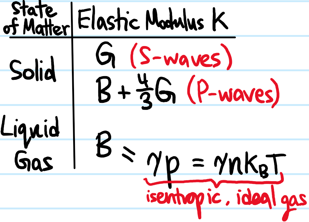
Problem: Define the specific acoustic impedance \(Z\) of a sound wave \(X(x,t)\) propagating in a non-dispersive medium (solid/liquid/gas) of density \(\rho\) with speed \(v\).
Solution: Similar to mechanical impedance except force is mapped to a pressure \(F\mapsto p\) to avoid dealing with the extensive nature of \(F\) depending on the area of application.
The pressure is \(p=-\rho c^2X’\) and the speed of the wave is \(\dot X\), so:
\[\dot X=\frac{-\rho c^2X’}{Z}\]
Either plug the travelling wave ansatz again \(X(x,t)=X(x-ct)\), or (equivalently) work in Fourier space:
\[-i\omega=\frac{-\rho c^2ik}{Z}\Rightarrow Z=\rho c\]
To make it look more like the violin string, one can write:
\[c=\frac{\rho c^2}{Z}=\sqrt{\frac{K}{\rho}}\]
where \(K\) is a suitable elastic modulus that depends on the type of wave and medium:
Problem: Define the electromagnetic impedance \(Z\) of a propagating EM wave in some medium (free space, dielectric, conductor, etc.)
Solution: The general definition is:
\[H=\frac{E}{Z}\]
where of course \(E:=|\textbf E|\) and \(H:=|\textbf H\) are the orthogonal \(\textbf E\) and \(\textbf H\)-fields. Invoking the constitutive relation \(E=v\times \mu H\) in a linear dielectric gives:
\[Z=\sqrt{\frac{\mu}{\varepsilon}}\]
Of course this applies to a conductor where \(\varepsilon\mapsto\varepsilon_{\text{eff}}=\varepsilon+i\sigma/\omega\).
Problem: Define the electrical impedance \(Z\) of a lumped element in an electric circuit.
Solution: This is Ohm’s law:
\[I=\frac{V}{Z}\]
(the connection with waves is a bit hazy here?)
Problem: Define the characteristic impedance of a transmission line with inductance per unit length \(\hat L\) and capacitance per unit length \(\hat C\), series resistance per unit length \(\hat R\), and parallel conductance per unit length \(\hat G\).
Solution:
\[Z=\sqrt{\hat R+i\omega\hat L}{\hat G+i\omega\hat C}\]
In the lossless case \(\hat R=\hat G=0\), this simplifies to:
\[Z=\sqrt{\frac{\hat L}{\hat C}}\]
Problem: Now that the notion of an impedance has been defined for a bunch of scenarios,
Problem: Explain why, in all the cases considered, the notion of a wave impedance \(Z\)
Impedance helps with steady-state calculations, comes from a linear constitutive law/equation of state/is intrinsic to a medium.
Problem:
Solution: Don’t memorize:
\[r=\frac{Z-Z’}{Z+Z’}\]
\[t=\frac{2Z}{Z+Z’}\]
One option is to memorize directly the interface matching conditions:
\[1+r=t\]
\[Z-Zr=Z’t\]
they are logically equivalent, but the latter makes it clear where it comes from. Furthermore, multiplying the latter \(2\) equations together yields the power flow/energy conservation equation:
\[Z(1-r^2)=Z’t^2\]
ensuring that \(R:=r^2\) and \(T:=\frac{Z’}{Z}t^2\) obey \(R+T=1\).
Alternatively, in direct analogy with “conservation of momentum” and “conservation of kinetic energy” from the context of elastic collisions, one can also remember the pair of equations:
\[Z=Zr+Z’t\]
\[\frac{1}{2}Z=\frac{1}{2}Zr^2+\frac{1}{2}Z’t^2\]
and similarly, the equation \(v+v’=V\) from that context directly translates to the continuity condition \(1+r=t\).
Problem: Explain why in some contexts (notably optics) the impedance looks “swapped”
Solution: Because of the mathematical identity:
\[\frac{Z’-Z}{Z+Z’}=\frac{\frac{1}{Z}-\frac{1}{Z’}}{\frac{1}{Z}+\frac{1}{Z’}}=\frac{Y-Y’}{Y+Y’}\]
in other words, it would have been more natural to work with the admittances.
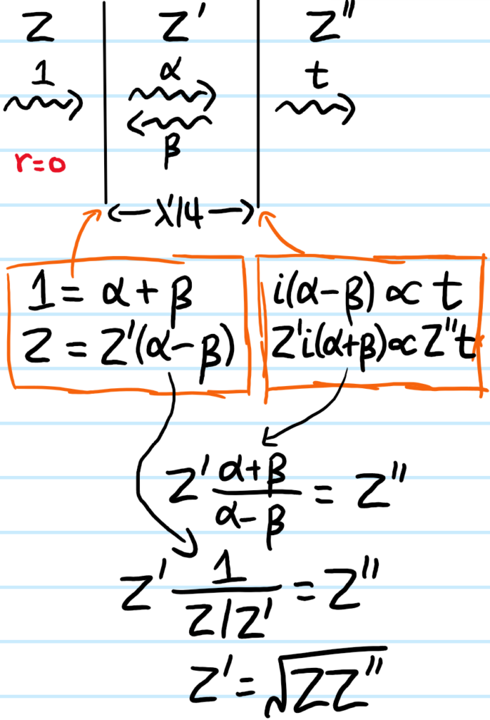
Problem: Impedance matching \(Z’=Z\) is desirable because it ensures that there are no reflections \(r=R=0\), i.e. perfect transmission \(t=T=1\). However, even if \(Z”\neq Z\), show that by inserting a length \(\lambda’/4\) of an intermediate medium with impedance \(Z’=\sqrt{ZZ”}\) the geometric mean, this acts to effectively impedance match anyways.
Solution: It is useful to first gain a heuristic understanding of this. Basically, the idea is that initially one has \(2\) media with mismatched impedances \(Z\neq Z^{\prime\prime}\); left like that, there would be reflections at the interface. So the idea is to insert an intermediate medium between the \(2\), where here the word “intermediate” not only means it’s literally intermediate between the \(2\) media, but also that its impedance \(Z’\) should be intermediate between the \(2\) (which will turn out to be the geometric mean). In other words, one is dealing with either a monotonically increasing or decreasing impedance “staircase”:
Then, when a wave is incident from the left, some of it will be reflected at the \(Z\neq Z’\) interface while some is transmitted. This transmitted light will then be incident on the \(Z’\neq Z^{\prime\prime}\) interface, and some of that will be reflected back towards the source, and get transmitted again through the original \(Z\neq Z’\) interface. Now, in order to eliminate any net back-reflection, one would like for \(2\) things to be true:
- The \(2\) reflections should interfere destructively, i.e. be \(\pi\) out of phase.
- Their amplitudes should also match up, so that one does indeed achieve complete destructive interference, rather than merely partial destructive interference.
Since there is a staircase setup, either both reflections got a \(\pi\)-phase shift or neither of them did. So in any case, this is basically nothing more than an application of thin film interference; the phase shift due to bouncing back and forth at normal incidence inside the intermediate medium of length \(L\) is:
\[\Delta\phi=k’2L=\pi+2\pi n\Rightarrow L=\left(\frac{1}{4}+\frac{n}{2}\right)\lambda’\]
with \(n=0\) being a common choice. As for the amplitude matching, unfortunately it doesn’t seem as straightforward to show that \(Z’=\sqrt{ZZ^{\prime\prime}\), since that does not imply:
\[\frac{Z-Z’}{Z+Z’}\neq\frac{2Z}{Z+Z’}\frac{Z’-Z^{\prime\prime}}{Z+Z^{\prime\prime}}\frac{2Z’}{Z+Z’}\]
(so it seems the tedious approach from matching boundary conditions is necessary? this is the quickest way I can think of for doing it with boundary conditions:)
Problem: Explain why megaphones are shaped like so:

Solution: