
Problem: What does it mean for \(N=2\) particles to be identical?
Solution: \(N=2\) particles are identical iff their intrinsic properties are all identical; in classical mechanics this typically means mass \(m\), charge \(q\), etc. while in quantum mechanics this typically means mass \(m\), charge \(q\), and spin \(s\) (and other intrinsic quantum numbers). The word intrinsic is important here. For example, \(2\) electrons are considered identical classical particles even if they are at different positions \(\textbf x_1\neq\textbf x_2\), or travelling with different velocities \(\dot{\textbf x}_1\neq\dot{\textbf x}_2\), and likewise are considered identical quantum particles even if they are in different quantum states \(|n,\ell,m_{\ell},m_s\rangle\neq |n’,\ell’,m_{\ell’},m_{s’}\rangle\) for instance (although exactly what properties qualify as “intrinsic” isn’t obvious a priori…)
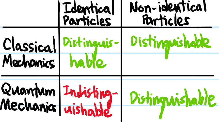
Problem: Fill in the \(4\) entries of the following \(2\times 2\) matrix with either the word distinguishable or indistinguishable.
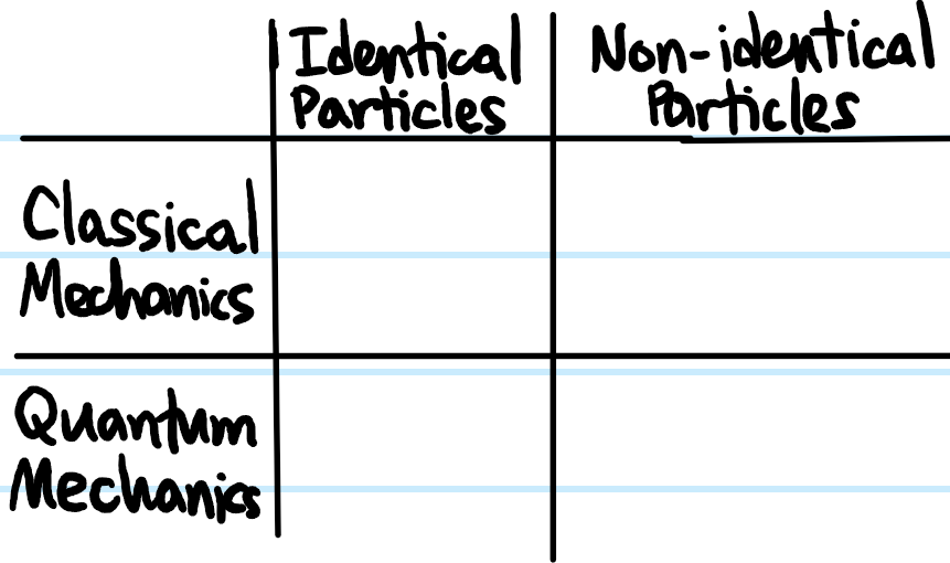
Solution:
Problem: Consider \(N=2\) identical quantum particles, thus described by a state in \(\mathcal H^{\otimes 2}\), where \(\mathcal H\) is each of their (identical) single-particle state space. Define the exchange operator \((12):\mathcal H^{\otimes 2}\to \mathcal H^{\otimes 2}\).
Solution: For some reason the term “exchange” is conventional in the QM literature even though the term “transposition” is usually used to describe this (e.g. in group theory). For unentangled states, the exchange operator is defined by:
\[(12)|\psi\rangle\otimes|\phi\rangle:=|\phi\rangle\otimes |\psi\rangle\]
where \(|\psi\rangle,|\phi\rangle\in\mathcal H\) are arbitrary single-particle states, and extended to the rest of \(\mathcal H^{\otimes 2}\) by linearity. In particular, transposition is manifestly independent of one’s choice of \(\mathcal H\)-basis because this definition doesn’t mention any \(\mathcal H\)-basis.
Problem: Show that \((12)\) is both unitary and Hermitian; hence what are the eigenvalues of \((12)\) and give an example of an eigenstate with each eigenvalue.
Solution:
The eigenvalues of \((12)\) are thus \(\text{spec}(12)=\{-1,1\}\). For example, \((12)|\psi\rangle\otimes|\psi\rangle=|\psi\rangle\otimes|\psi\rangle\) has eigenvalue \(1\) for any \(|\psi\rangle\in\mathcal H\). By contrast, \((12)(|\psi\rangle\otimes|\phi\rangle-|\phi\rangle\otimes|\psi\rangle)=-(|\psi\rangle\otimes|\phi\rangle-|\phi\rangle\otimes|\psi\rangle)\) has eigenvalue \(-1\) for any \(|\psi\rangle,|\phi\rangle\in\mathcal H\)
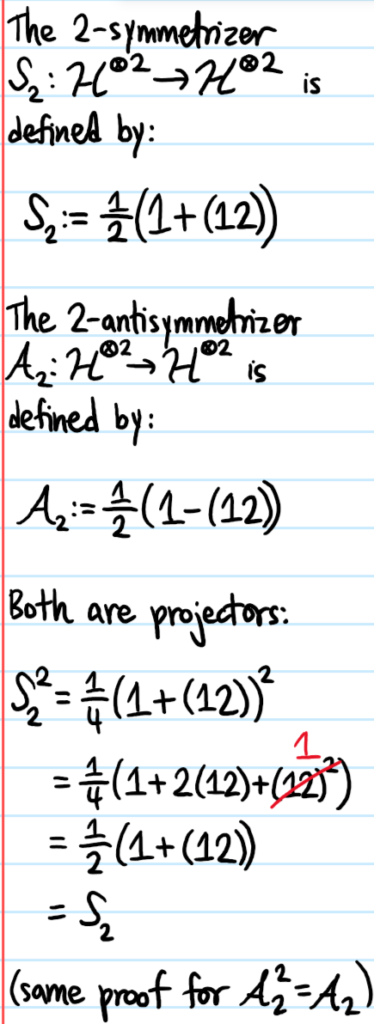
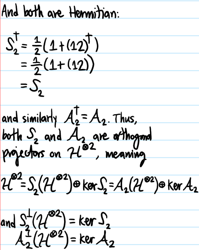
Problem: Define the \(2\)-symmetrizer \(\mathcal S_2\) and the \(2\)-antisymmetrizer \(\mathcal A_2\) and show that both are orthogonal projectors.
Solution:
Problem: Let \(A,B:\mathcal H\to\mathcal H\) each be arbitrary linear operators on the single-particle state space \(\mathcal H\). The exchange operator acts on states by a unitary \((12)\) which swaps \(|\psi\rangle\otimes|\phi\rangle\mapsto|\psi\rangle\otimes|\phi\rangle\). If one wished to achieve an analogous result at the level of operators, specifically \(A\otimes B\mapsto B\otimes A\), how can this be accomplished?
Solution:

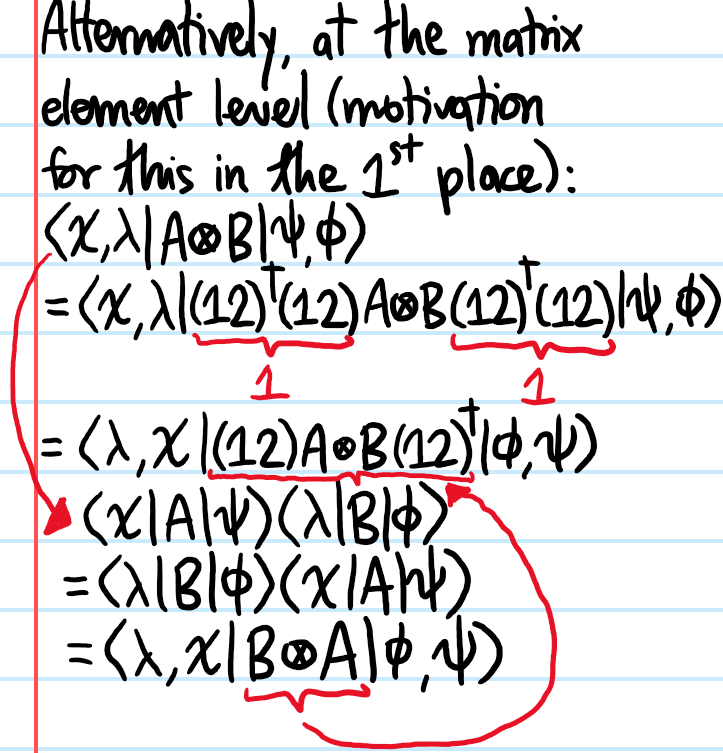
Problem: Generalizing the above slightly, given arbitrarily many compositions of operators on \(\mathcal H^{\otimes 2}\), e.g. \((A\otimes B)(C\otimes D)(E\otimes F)…\), how can one obtain the operator \((B\otimes A)(D\otimes C)(F\otimes E)…\)?
Solution: Do exactly what was done above:
\[(12)(A\otimes B)(C\otimes D)(E\otimes F)…(12)^{-1}\]
\[=(12)(A\otimes B)(12)^{-1}(12)(C\otimes D)(12)^{-1}(12)(E\otimes F)(12)^{-1}(12)…(12)^{-1}\]
\[=(B\otimes A)(D\otimes C)(F\otimes E)…\]
Problem: Show that an operator \(\mathcal O:\mathcal H^{\otimes 2}\to\mathcal H^{\otimes 2}\) is exchange-symmetric iff \([\mathcal O,(12)]=0\).
Solution: In light of the above, an exchange-symmetric operator is reasonably defined to obey:
\[(12)\mathcal O(12)^{-1}=\mathcal O\]
and hence the result follows.
(aside: all of the above discussion also holds for \(2\) non-identical quantum particles provided one assumes they are each described by the same single-particle state space \(\mathcal H\)).
Now, generalize the prior discussion to an arbitrary number \(N\) of identical quantum particles.
Problem: Define the \(N\)-symmetrizer \(\mathcal S_N\) and the \(N\)-antisymmetrizer \(\mathcal A_N\) operators on the space \(\mathcal H^{\otimes N}\) of \(N\) identical particles (where \(\mathcal H\) as before is the single-particle state space).
Solution: The \(N\)-symmetrizer is defined by:
\[\mathcal S_N:=\frac{1}{\#S_N}\sum_{\sigma\in S_N}\sigma\]
And the \(N\)-antisymmetrizer is defined by:
\[\mathcal A_N:=\frac{1}{\#S_N}\sum_{\sigma\in S_N}\text{sgn}(\sigma)\sigma=\frac{1}{\#S_N}\left(\sum_{\sigma\in A_N}\sigma-\sum_{\sigma\in S_N-A_N}\sigma\right)\]
where \(\#S_N=N!\), and note this is consistent with the earlier definitions for \(N=2\). Strictly speaking each permutation \(\sigma\in S_N\) is an abstract group element for which there is no notion of “group addition”, rather this is a faithful unitary representation of \(S_N\) on \(\mathcal H^{\otimes N}\) (a more pedantic notation could be \(\hat{\sigma}\) for the permutation operator associated to \(\sigma\)).
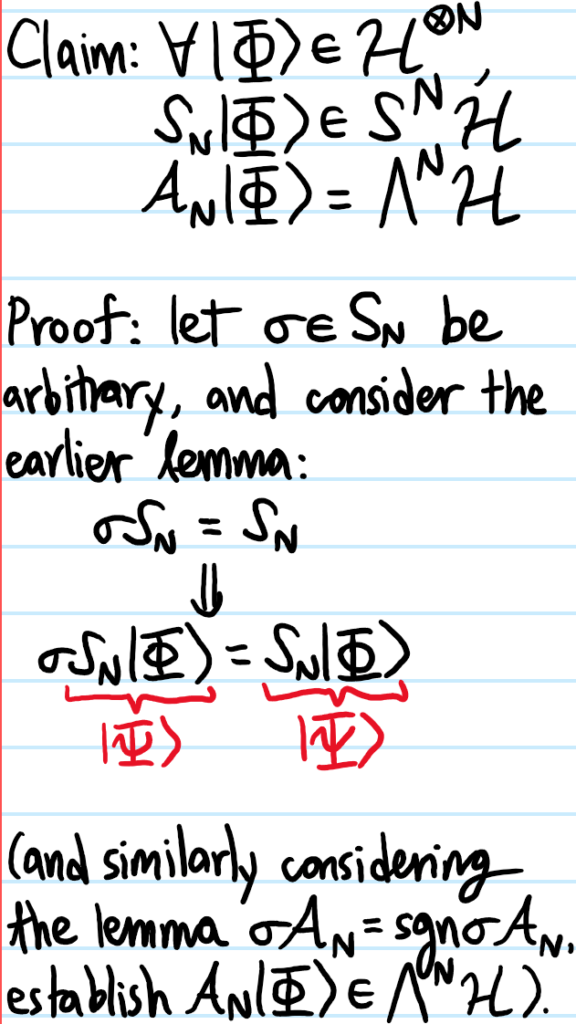
Problem: Establish the following properties of \(\mathcal S_N\) and \(\mathcal A_N\):
i) (Useful lemma) \[\sigma\mathcal S_N=\mathcal S_N\sigma=\mathcal S_N\] and \[\sigma\mathcal A_N=\mathcal A_N\sigma=\text{sgn}(\sigma)\mathcal A_N\] for any \(\sigma\in S_N\).
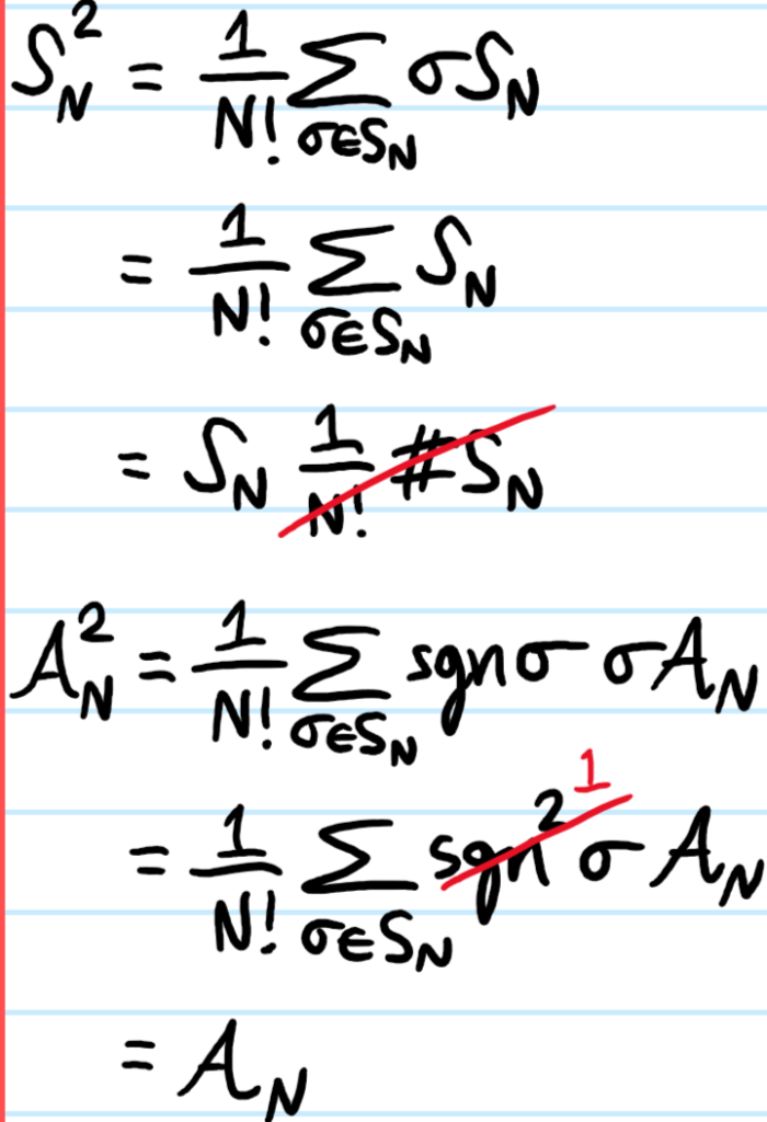
ii) (Orthogonal projectors) \(\mathcal S^2_N=\mathcal S_N\) and \(\mathcal A^2_N=\mathcal A_N\) are both idempotent projections, and \(\mathcal S^{\dagger}_N=\mathcal S_N\) and \(\mathcal A^{\dagger}_N=\mathcal A_N\) are both Hermitian observables.
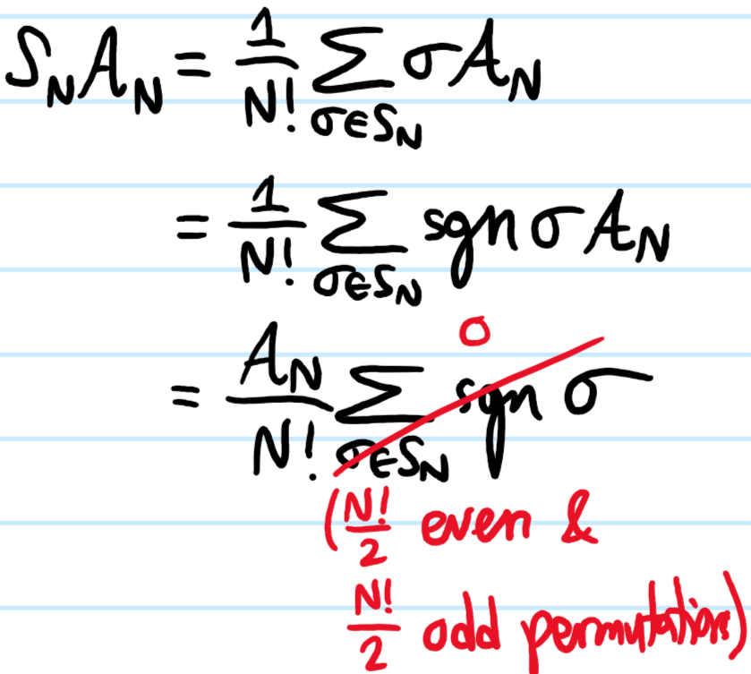
iii) (Orthogonal images) \(\mathcal S_N\mathcal A_N=\mathcal A_N\mathcal S_N=0\) (but note this is in general not a full orthogonal complement, i.e. \((\mathcal S^{\perp}_N(\mathcal H^{\otimes N})\neq\mathcal A_N(\mathcal H^{\otimes N})\) unless \(N=2\); in other words, for \(N\geq 3\), there exist states that are neither symmetric nor antisymmetric, but have mixed symmetries, see Young tableaux).
Solution:
i) Since \(S_N\) is a normal subgroup of itself, its left/right cosets coincide and indeed, all simply return \(S_N\) trivially. For \(\mathcal A_N\), one can write:
\[\sigma\mathcal A_N=\frac{1}{N!}\sum_{\hat{\sigma}\in S_N}\text{sgn}(\hat{\sigma})\sigma\hat{\sigma}\]
\[=\frac{1}{N!}\sum_{\hat{\sigma}\in S_N}\text{sgn}(\hat{\sigma})\text{sgn}^2(\sigma)\sigma\hat{\sigma}\]
\[=\frac{\text{sgn}(\sigma)}{N!}\sum_{\hat{\sigma}\in S_N}\text{sgn}(\hat{\sigma})\text{sgn}(\sigma)\sigma\hat{\sigma}\]
and since \(\text{sgn}:S_N\to\{-1,1\}\) is a homomorphism, this simplifies to the claimed result.
ii) First, note that (as mentioned above), all permutations \(\sigma\in S_N\) are unitary (this follows because all permutations can be built from transpositions alone, each of which was proven to be unitary from the \(N=2\) analysis earlier). Thus, taking the adjoint is the same as the inverse. So:
\[\mathcal S^{\dagger}_N=\frac{1}{N!}\sum_{\sigma\in S_N}\sigma^{\dagger}\]
\[=\frac{1}{N!}\sum_{\sigma\in S_N}\sigma^{-1}\]
but \(S_N\) is a group, so inversion is a group bijection, and the sum is invariant. For \(\mathcal A_N\), the proof of Hermiticity is almost identical with the additional insight that inversion also preserves the sign \(\text{sgn}(\sigma^{-1})=\text{sgn}(\sigma)\) since any decomposition into transpositions would just be reversed, but the number of transpositions (even/odd) would be invariant. Regarding projection:
iii) For example:
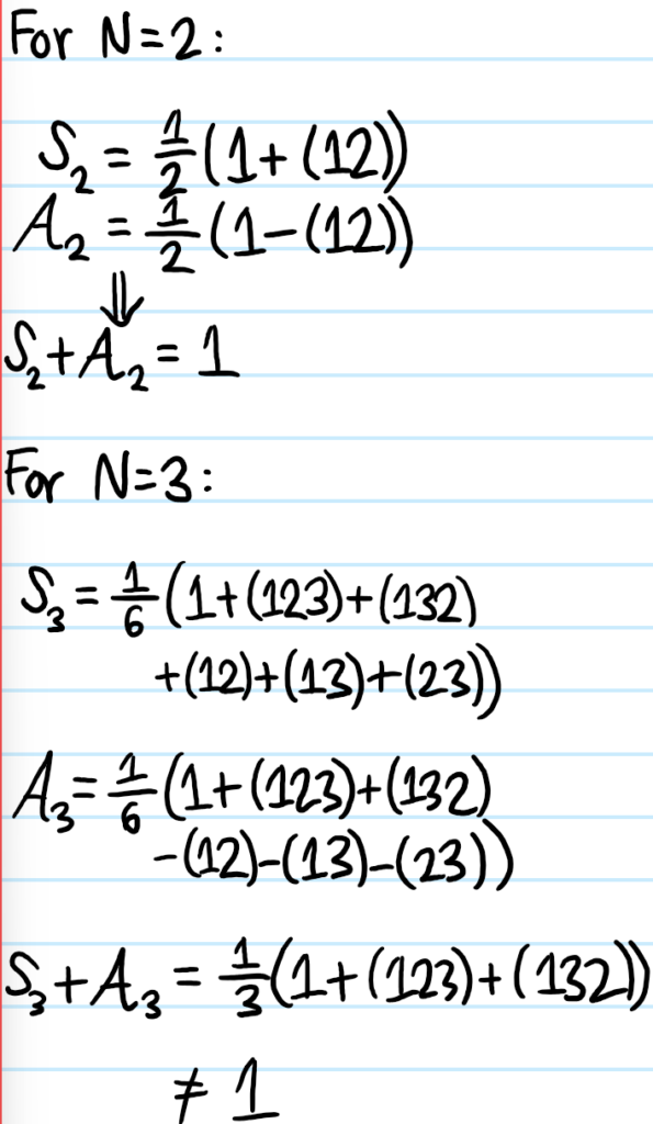
Problem: Following up on the above iii), show explicitly that for \(N=2\) identical particles, \(S_2+A_2=1\) partitions the space \(\mathcal H^{\otimes 2}\) but for \(N=3\) identical particles \(S_3+A_3\neq 1\).
Solution: (it seems the reason it breaks down is basically because for \(N\geq 3\), the identity permutation is no longer the only even permutation)
Problem: Define the totally symmetric state subspace \(S^N\mathcal H\) and the totally antisymmetric state subspace \(\bigwedge^N\mathcal H\) of the full \(N\)-particle state space \(\mathcal H^{\otimes N}\) and hence explain why the \(N\)-symmetrizer \(\mathcal S_N:\mathcal H^{\otimes N}\to S^N\mathcal H\) and the \(N\)-antisymmetrizer \(\mathcal A_N:\mathcal H^{\otimes N}\to \bigwedge^N\mathcal H\) may be viewed thus.
Solution: The totally symmetric state subspace is essentially the intersection of the eigenspaces of all permutation operators with eigenvalue \(1\) (or in group-theoretic language, the set of all states whose stabilizer subgroup is \(S_N\) itself):
\[S^N\mathcal H:=\{|\Psi\rangle\in\mathcal H^{\otimes N}:\sigma|\Psi\rangle=|\Psi\rangle\text{ for all }\sigma\in S_N\}\]
(permutation operators do not commute as one can see from the conjugacy classes of \(S_N\), so they cannot all be simultaneously diagonalized, but nevertheless it turns out to still be possible to find special symmetric states that are eigenstates of all of them). The totally antisymmetric state subspace is defined by:
\[\bigwedge^N\mathcal H:=\{|\Psi\rangle\in\mathcal H^{\otimes N}:\sigma|\Psi\rangle=\text{sgn}(\sigma)|\Psi\rangle\text{ for all }\sigma\in S_N\}\]
Problem: State the symmetrization postulate of quantum mechanics.
Solution: For a system of \(N\) identical quantum particles, not all states in \(\mathcal H^{\otimes N}\) are physical states, even though they may be valid “mathematical states”. Instead, only states in \(S^N\mathcal H\) xor states in \(\bigwedge^N\mathcal H\) can be physical states, corresponding respectively to identical bosons vs. identical fermions.
Problem: Show that for any \(N\)-body state \(|\Psi\rangle\in\mathcal H^{\otimes N}\), the symmetrization of \(|\Psi\rangle\) obtained by acting with the \(N\)-symmetrizer \(\mathcal S_N|\Psi\rangle\) is unique in the projective totally symmetric state subspace \(PS^N\mathcal H\), and similarly the antisymmetrization of \(|\Psi\rangle\) obtained by acting with the \(N\)-antisymmetrizer \(\mathcal A_N|\Psi\rangle\) is unique in \(P\bigwedge^N\mathcal H\).
Solution: One can proceed by demonstrating that:
\[\text{span}_{\textbf C}S_N|\Psi\rangle\cap S^N\mathcal H=\text{span}_{\textbf C}\mathcal S_N|\Psi\rangle\]
\[\text{span}_{\textbf C}S_N|\Psi\rangle\cap \bigwedge^N\mathcal H=\text{span}_{\textbf C}\mathcal A_N|\Psi\rangle\]
For example, for the \(2^{\text{nd}}\) assertion above:
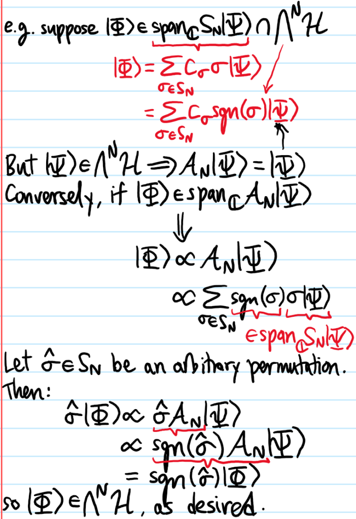
and the proof the first one is similar. Intuitively, any linear combination of permutations which is symmetric must in fact give uniform weight to all permutations (which is what \(\mathcal S_N\) prescribes), and similarly if the linear combination is antisymmetric, then each permutation is weighted by its sign instead (as per \(\mathcal A_N\)).
Problem: Let \(\{|1\rangle,|2\rangle,…\}\subseteq\mathcal H\) be an orthonormal basis of the single-particle state space \(\mathcal H\), and consider \(N\) identical particles living collectively in \(\mathcal H^{\otimes N}\). Explain why it is useful to introduce the notation \(|N_1,N_2,…,\rangle\) (called the occupation number representation) to denote that there are \(N_i\in\textbf N\) particles in single-particle state \(|i\rangle\in\mathcal H\).
Solution: Because the particles are identical, it is highly inefficient to be asking “which state is which particle in” since the notion of “which particle” is meaningless. Instead, common sense dictates that the more efficient question to ask is “how many particles are in each state?” as this doesn’t care about which particle is which.
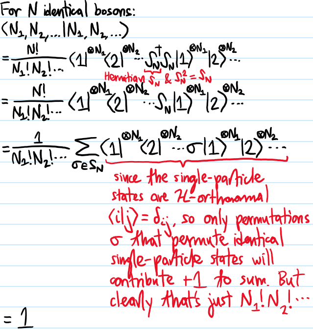
Problem: If one demands \(\langle N_1,N_2,…|N_1,N_2,…\rangle=1\) to be normalized, then write down a single unified formula for \(|N_1,N_2,…\rangle\) in the language of first quantization that works regardless of whether the particles are identical bosons or identical fermions.
Solution: A little bit of thought shows that one possibility is:
\[|N_1,N_2,…\rangle=\frac{1}{\sqrt{N!N_1!N_2!…}}\sum_{\sigma\in S_N}(\pm)^{(1-\text{sgn}(\sigma))/2}\sigma|1\rangle^{\otimes N_1}|2\rangle^{\otimes N_2}…\]
where \(N=N_1+N_2+…\), and the \(\pm\) should be taken as \(+\) for bosons and \(-\) for fermions. If it’s for \(N\) identical bosons, one can write it in terms of the \(N\)-symmetrizer:
\[|N_1,N_2,…\rangle=\sqrt{\frac{N!}{N_1!N_2!…}}\mathcal S_N|1\rangle^{\otimes N_1}|2\rangle^{\otimes N_2}…\]
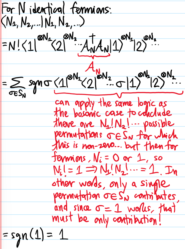
while for \(N\) identical fermions, the Pauli exclusion principle enforces \(N_i\in\{0,1\}\) for all single-particle states \(|i\rangle\), and thus \(N_i!=1\). Thus, in this case:
\[|N_1,N_2,…\rangle=\sqrt{N!}\mathcal A_N|1\rangle^{\otimes N_1}|2\rangle^{\otimes N_2}…\]
One can explicitly check the normalization of the state written in this manner:
Problem: Consider a system of \(3\) hydrogen atoms, \(2\) of which are in a single-particle ground state \(|0\rangle\) and \(1\) of them is in some single-particle excited state \(|1\rangle\); write down the \(3\)-body collective state of this system in first quantization.
Solution: Phrases like “ground state” and “excited state” are simply particular eigenstates of the single-particle Hamiltonian \(H\); in particular, because \(H\) is Hermitian, these single-particle states may be taken orthonormal. With this in mind, because hydrogen atoms are bosons (assuming the usual protium isotope without neutrons), the occupation number state \(|N_{|0\rangle}=2,N_{|1\rangle}=1\rangle\) is given in first quantization by:
\[|N_{|0\rangle}=2,N_{|1\rangle}=1\rangle=\frac{1}{\sqrt{3!2!1!}}(|001\rangle+|001\rangle+|010\rangle+|010\rangle+|100\rangle+|100\rangle)\]
\[=\frac{|001\rangle+|010\rangle+|100\rangle}{\sqrt 3}\]
where of course the shorthand \(|001\rangle:=|0\rangle\otimes |0\rangle\otimes |1\rangle\), etc. is being used.
Problem: All of the above discussion is always prefaced by fixing the number of identical quantum particles \(N\); in other words, all of the physics happens inside the \(N\)-particle sector of the Fock space \(\mathcal F_{\mathcal H}\) generated by the single-particle state space \(\mathcal H\). Define the Fock space \(\mathcal F_{\mathcal H}\) for identical bosons, and separately for identical fermions.
Solution: For both bosons and fermions, one can write:
\[\mathcal F_{\mathcal H}:=\bigoplus_{N=0}^{\infty}\text{span}_{\textbf C}\{|N_1,N_2,…\rangle:N_1+N_2+…=N\}\]
But it is clearer to distinguish between the bosonic Fock space:
\[\mathcal F_{\mathcal H}=\bigoplus_{N=0}^{\infty}S^N\mathcal H\]
and the fermionic Fock space:
\[\mathcal F_{\mathcal H}=\bigoplus_{N=0}^{\infty}\bigwedge^N\mathcal H\]
(in fact the fermionic Fock space can also be written \(\mathcal F_{\mathcal H}=\bigoplus_{N=0}^{\dim\mathcal H}\bigwedge^N\mathcal H\) since for \(N>\dim\mathcal H\), the totally antisymmetric state space \(\bigwedge^N\mathcal H=\{0\}\) is trivial).
Problem: Explain why the Fock space \(\mathcal F_{\mathcal H}\) needs to be formed by a direct sum \(\oplus_{N=0}^{\infty}\) rather than just a union \(\bigcup_{N=0}^{\infty}\). Furthermore, explain how to complete Fock space \(\mathcal F_{\mathcal H}\) into a Hilbert space by explicitly stating the inner product placed on \(\mathcal F_{\mathcal H}\).
Solution: Simply put, the union \(\bigcup_{N=0}^{\infty}\) doesn’t preserve the vector space structure, hence the need for the direct sum \(\oplus_{N=0}^{\infty}\). The canonical inner product on \(\mathcal F_{\mathcal H}\) is defined by summing the inner product between respective components in the \(N\)-particle sectors (this statement is just a general property of direct sums in linear algebra).
Problem: Clarify by the above discussion by working through the example of electrons fixed in space, so that \(\mathcal H\cong\textbf C^2\). Let \(|0\rangle,|1\rangle\) be an orthonormal basis for \(\mathcal H\). What is the electron Fock space \(\mathcal F_{\mathcal H}\)? What is its dimension \(\dim(\mathcal F_{\mathcal H})\)? What is a basis for \(\mathcal F_{\mathcal H}\)? Hence, show that distinct \(N\)-particle sectors are orthogonal.
Solution:
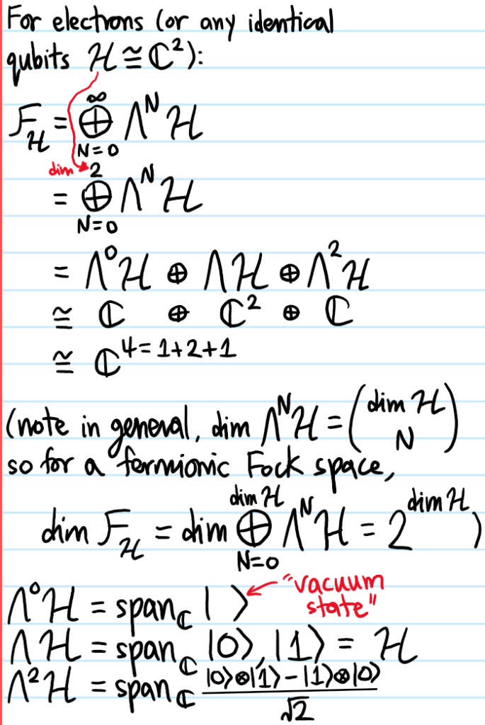
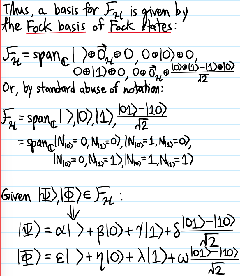
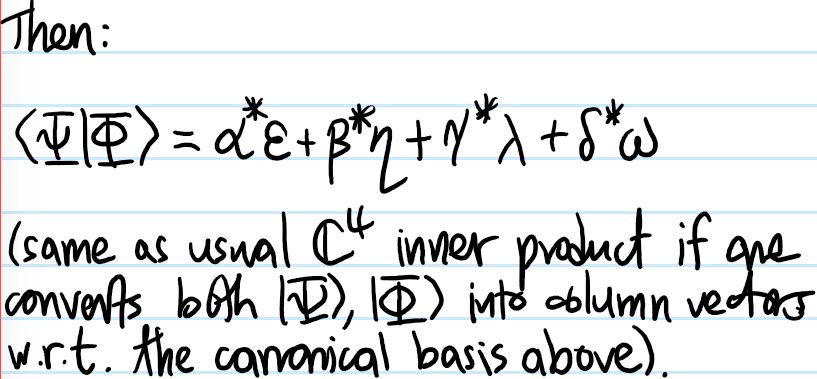
in particular, it is clear that distinct \(N\)-particle sectors are orthogonal because the Fock states here \(|\space\rangle,|0\rangle,|1\rangle,\frac{|01\rangle-|10\rangle}{\sqrt{2}}\) form an orthonormal basis for \(\mathcal F_{\mathcal H}\cong\textbf C^4\). Note that both \(|\Psi\rangle,|\Phi\rangle\) will (in general) not be called Fock states because they do not contain a fixed number of particles \(N\), but rather are said to be in a superposition of Fock states, each of which by definition only deals with a fixed number \(N\) of particles in some \(N\)-particle sector (which is why it could be written using a single occupation number ket).
Problem: Outside of QFT, particles are conserved \(\dot N=0\), so it’s not obvious why one would ever want to somehow “tamper” with the number of particles \(N\) in the system. Nevertheless, it turns out to be very useful, like a magician waving their magic wand to make rabbits appear or disappear from their hat. Explain how the creation and annihilation operators for bosons and fermions are defined respectively on the bosonic and fermionic Fock spaces \(\mathcal F_{\mathcal H}\).
Solution: For a given single-particle basis \(\{|i\rangle\}\subset\mathcal H\) of the single-particle state space \(\mathcal H\), to each single-particle basis ket \(|i\rangle\), one associates a creation operator \(a^{\dagger}_i:\mathcal F_{\mathcal H}\to\mathcal F_{\mathcal H}\) and similarly an annihilation operator \(a_i:\mathcal F_{\mathcal H}\to\mathcal F_{\mathcal H}\). Since Fock states \(|N_1,N_2,…,\rangle\) form a basis for the Fock space \(\mathcal F_{\mathcal H}\), to define the action of each \(a^{\dagger}_i,a_i\) on the full Fock space \(\mathcal F_{\mathcal H}\), it suffices to define their actions on each Fock state, and extend to the rest of \(\mathcal F_{\mathcal H}\) by linearity. Hence, they are defined to act on Fock states via:
\[a^{\dagger}_i|N_1,N_2,…,N_i,…\rangle=\sqrt{N_i+1}|N_1,N_2,…,N_i+1,…\rangle\]
\[a_i|N_1,N_2,…,N_i,…\rangle=\sqrt{N_i}|N_1,N_2,…,N_i-1,…\rangle\]
However, one should check that these \(2\) definitions are compatible in the sense that the claimed adjoint relation between \(a^{\dagger}_i\) and \(a_i\) is really correct w.r.t. the Fock space inner product. To this end, one has to check that for arbitrary \(|\Psi\rangle,|\Phi\rangle\in\mathcal F_{\mathcal H}\):
\[\langle\Psi|a^{\dagger}_i|\Phi\rangle=\langle\Phi|a_i|\Psi\rangle^*\]
but bilinearity of the inner product means it suffices to check this when \(|\Psi\rangle=|N_1,N_2,…,N_i,…\rangle\) and \(|\Phi\rangle=|N’_1,N’_2,…,N’_i,…\rangle\) are both Fock states:
\[\langle N_1,N_2,…,N_i,…|a^{\dagger}_i|N’_1,N’_2,…,N’_i,…\rangle\]
\[=\sqrt{N’_i+1}\langle N_1,N_2,…,N_i,…|N’_1,N’_2,…,N’_i+1,…\rangle\]
\[=\sqrt{N’_i+1}\delta_{N_1,N’_1}\delta_{N_2,N’_2}…\delta_{N_i,N’_i+1}…\]
On the other hand:
\[\langle N’_1,N’_2,…,N’_i,…|a_i|N_1,N_2,…,N_i,…\rangle^*\]
\[=\sqrt{N_i}\langle N’_1,N’_2,…,N’_i,…|N_1,N_2,…,N_i-1,…\rangle^*\]
\[=\sqrt{N_i}\delta_{N’_1,N_1}\delta_{N’_2,N_2}…\delta_{N’_i,N_i-1}…\]
which are clearly the same expression.
Problem: Complete the following tasks:
i) Write down a formula for a generic Fock state \(|N_1,N_2,…,\rangle\) in terms of creation operators acting on the vacuum \(|\space\rangle=|N_1=0,N_2=0,…\rangle\).
ii) Explain why, for any single-particle state \(|i\rangle\in\mathcal H\), the \(\alpha=0\) coherent state is given by:
\[\text{ker}a_i=\text{span}_{\textbf C}\{|N_1,N_2,…,N_i=0,…\rangle\in\mathcal F_{\mathcal H}\}\]
iii) Evaluate for bosons the commutators \([a_i,a_j],[a^{\dagger}_i,a^{\dagger}_j],[a_i,a^{\dagger}_j]\) and for fermions the anticommutators \(\{c_i,c_j\},\{c^{\dagger}_i,c^{\dagger}_j\},\{c_i,c^{\dagger}_j\}\) (for fermions it is conventional to use the letter “\(c\)” in lieu of “\(a\)”).
iv) Given \(2\) single-particle bases \(\{|i\rangle\}\) and \(\{|\tilde i\rangle\}\) for the single-particle state space \(\mathcal H\), explain how to relate \(a^{\dagger}_i\) with \(a^{\dagger}_{\tilde i}\) and similarly how to relate \(a_i\) with \(a_{\tilde i}\). Verify that these transformations preserve the commutation/anticommutation relations.
v) Define the number operator \(\hat N_i\) and show that when acting on a Fock state, it counts the number of identical particles in the single-particle state \(|i\rangle\) (in fact, a good way to think about Fock states is that they are eigenstates of the total number operator \(\hat N:=\sum_i\hat N_i\)).
Solution:
i) In second quantization, the Fock state is given by:
\[|N_1,N_2,…,\rangle=\]
ii)
iii)
iv) Although it is tempting to think of this as a “change of basis” from linear algebra, this is actually not what’s going on…(or is it?)
v)
Problem: For \(\mathcal H=L^2(\textbf R^3\to\textbf C)\), one can use either the orthonormal \(\textbf X\)-eigenbasis \(\{|\textbf x\rangle\}\) or the orthonormal\(\textbf P\)-eigenbasis \(\{|\textbf k\rangle\). Show that the corresponding creation and annihilation operator fields for each are related by a Fourier transform:
\[\psi^{\dagger}(\textbf x):=a^{\dagger}_{\textbf x}\]
\[\]
where the notation \(\psi(\textbf x):=a_{\textbf x}\) and \(\psi_{\textbf k}:=a_{\textbf k}\) is being used (unambiguous with the wavefunction because this is \(2^{\text{nd}}\) quantization now! No more \(1^{\text{st}}\) quantization).
Problem: Consider a system of \(N=2\) identical non-interacting spin \(s=1/2\) fermions in an infinite potential well of width \(L\) (nodes at \(x=0,L\)). Write down the general \(2\)-body wavefunction \(\Psi(1,2)\) for the system’s ground state, \(1^{\text{st}}\) excited state, and \(2^{\text{nd}}\) excited state by calculating Slater determinants of the single-fermion spin-orbitals.
Solution: Use the notation \(\chi_{n,m_s}\) for the spin-orbital (note the word “orbital” here isn’t really meant in the sense of e.g. orbital angular momentum \(\textbf L\), but rather in the chemist sense of “atomic orbital” though the \(2\) notions aren’t entirely disjoint):
\[\chi_{n,m_s}=|\psi_n\rangle\otimes|m_s\rangle\]
where \(\psi_n(x)=\sqrt{\frac{2}{L}}\sin\frac{n\pi x}{L}\) is the position space wavefunction of the \(n^{\text{th}}\) excited single-particle state. Use the notation \(\chi_{n,m_s}(i)\) to refer to placing the (arbitrarily labelled) \(i^{\text{th}}\) fermion (\(i\in\{1,2\}\)) into the spin-orbital \(\chi_{n,m_s}\):
\[\chi_{7,\uparrow}(2)\cong \sqrt{\frac{2}{L}}\sin\frac{7\pi x_2}{L}|\uparrow\rangle_2\]
In this case, a general Slater determinant of spin-orbitals is of the form:
\[\Psi(1,2)=\frac{1}{\sqrt{2!}}\det\begin{pmatrix}\chi_{n_1,m^{(1)}_s}(1)&\chi_{n_2,m^{(2)}_s}(1)\\\chi_{n_1,m^{(1)}_s}(2)&\chi_{n_2,m^{(2)}_s}(2)\end{pmatrix}\]
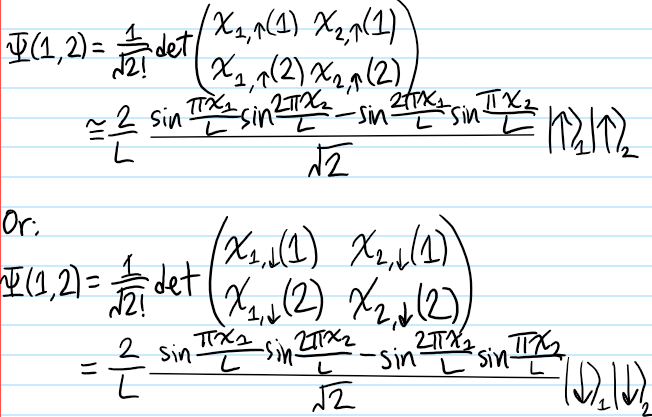
Now consider the ground state. Because the fermions are non-interacting, this amounts to the requirement \(n_1=n_2=1\), thus fixing the spatial part of the allowed spin-orbitals. In particular, since the spatial parts are identical, the spin parts cannot be \(m^{(1)}_s\neq m^{(2)}_s\) otherwise \(\Psi(1,2)=0\); this is just the Pauli exclusion principle. Arbitrarily letting \(m^{(1)}_s=-m^{(2)}_s=1/2\), it follows that the ground state manifold is one-dimensional, and spanned by the ground state:
\[\Psi(1,2)=\frac{1}{\sqrt{2!}}\det\begin{pmatrix}\chi_{1,\uparrow}(1)&\chi_{1,\downarrow}(1)\\\chi_{1,\uparrow}(2)&\chi_{1,\downarrow}(2)\end{pmatrix}\cong\frac{2}{L}\sin\frac{\pi x_1}{L}\sin\frac{\pi x_2}{L}\frac{|\uparrow\rangle_1|\downarrow\rangle_2-|\downarrow\rangle_1|\uparrow\rangle_2}{\sqrt{2}}\]
So the spatial part of the \(2\)-body wavefunction is clearly \(1\leftrightarrow 2\) symmetric while the singlet spin part is \(1\leftrightarrow 2\) antisymmetric, ensuring total antisymmetry \(\Psi(2,1)=-\Psi(1,2)\).
Meanwhile, for the system’s \(1^{\text{st}}\) excited state:
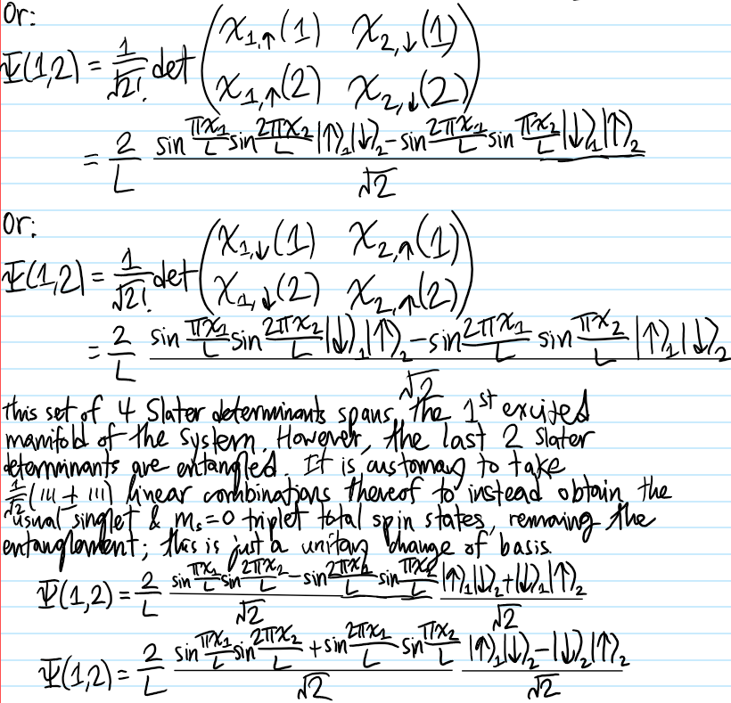
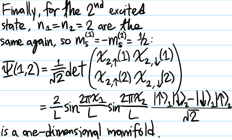
Problem: Briefly describe how the results above would be affected if instead it were \(N=2\) identical non-interacting spin \(s=1\) bosons.
Solution: Instead of Slater determinants, one would use “Slater permanents”, or just “permanents” for short. These are basically calculated in the same way as a determinant except all minus signs become plus signs. This implicitly enforces total symmetry \(\Psi(2,1)=\Psi(1,2)\) of the wavefunction. In addition, because \(2s+1=3\) now, the degeneracies of each manifold would be enhanced.
Problem: What is the explicit connection between the Slater permanents/determinants and the symmetrizer/antisymmetrizer?
Solution: The idea is to symmetrize/antisymmetrize the Hartree product ansatz, essentially providing the bridge to Hartree-Fock. This immediately yields Slater permanents/determinants respectively (up to a normalization):
\[\sqrt{N!}\mathcal S_N\chi_1(1)\chi_2(2)…\chi_N(N)=\frac{1}{\sqrt{N!}}\text{perm}\begin{pmatrix}\chi_1(1)\end{pmatrix}\]
(FILL IN THE PERM)
\[\sqrt{N!}\mathcal A_N\chi_1(1)\chi_2(2)…\chi_N(N)=\frac{1}{\sqrt{N!}}\text{det}\begin{pmatrix}\chi_1(1)\end{pmatrix}\]
(FILL IN THE DET)
Problem: The purpose of the previous problems wasn’t so much to actually compute all those \(N\)-body wavefunctions \(\Psi(1,…,N)\), but rather to force one to compute them in order to realize how tedious and redundant the whole business is.
A warning: second quantization is only really useful for systems of identical particles; if the \(N\) particles were all distinguishable then in principle one can still use the second quantization framework, but in that case it doesn’t offer any advantage over just plain wavefunction language (aka first quantization).
Problem: Derive the commutation relations for the bosonic creation/annihilation operators and similarly derive the anticommutation relations for the fermionic creation/annihilation operators, starting from … . This shows that commutation and anticommutation relations completely encode the permutation symmetries of the bosonic and fermionic states.
Problem: What does it mean for a linear operator \(H\) to be an \(N\)-body operator?
Solution: An operator \(H\) is said to be an \(N\)-body operator iff there exists a decomposition of \(H\) in the form:
\[H=\sum_i H_i\]
where each operator \(H_i\) acts only on \(N\) particles at a time, acting as the identity operator on all other particles. For instance, the kinetic energy operator for an arbitrary system of particles (whether identical or not) is a \(1\)-body operator, as are most external potentials. By contrast, common \(2\)-body operators include interaction potentials between particles.
Problem: Given a system of \(N\) identical particles (fermions or bosons), and a \(1\)-body operator \(H\), and a basis \(\{|i\rangle\}\) of the single-particle Hilbert space, explain why the second quantization functor acting on \(H\) is given by the “dictionary”:
\[|i\rangle\mapsto c^{\dagger}_{|i\rangle}|\space\rangle\]
\[H\mapsto\sum_{|i\rangle,|j\rangle}\langle i|H|j\rangle c^{\dagger}_{|i\rangle}c_{|j\rangle}\]
Solution: Because the matrix elements are preserved under this homomorphism, so the functor is sort of “unitary” in a way? More precisely, matrix elements between any \(2\) Fock states are unchanged.
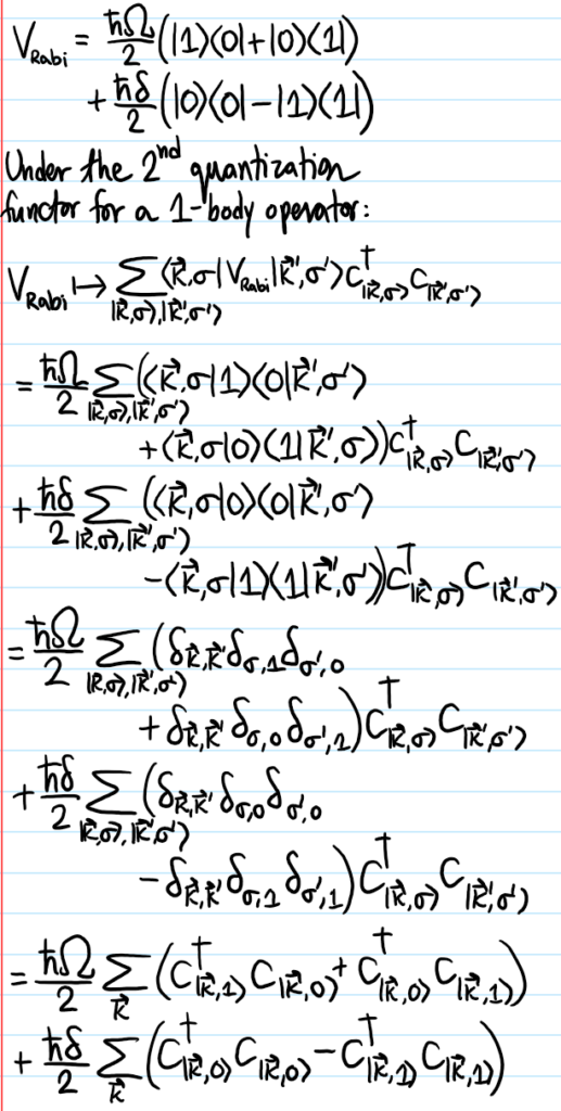
Problem: Write the one-body Rabi drive operator \(V_{\text{Rabi}}=\frac{\hbar}{2}\tilde{\boldsymbol{\Omega}}\cdot\boldsymbol{\sigma}\) in \(2^{\text{nd}}\) quantization.
Solution: Since the states \(\{|\textbf k,\sigma\rangle\}\) are a basis for the single-particle Hilbert space:
Problem: Write the \(2\)-body scattering contact pseudopotential operator \(V:=g\delta^3(\textbf X-\textbf X’)\) in \(2^{\text{nd}}\) quantization.