Problem: Given a linear operator \(H\) on some vector space, define the resolvent operator \(G_H(E)\) associated to \(H\).
Solution: The resolvent \(G_H(E)\) of \(H\) is the operator-valued Mobius transformation of a complex variable \(E\in\textbf C\) defined by the inverse:
\[G_H(E):=\frac{1}{E1-H}\]
(this notation \(A/B\) is only unambiguous when \([A,B^{-1}]=0\) which it is in this case).
Problem: What is the domain for \(E\in\textbf C\) of the resolvent \(G_H(E)\)?
Solution: Any value of \(E\in\textbf C\) for which the matrix \(E1-H\) is invertible leads to a well-defined resolvent. But invertibility is equivalent to a non-vanishing determinant \(\det(E1-H)\neq 0\). However, when \(\det(E1-H)=0\), then \(E\) is an eigenvalue of \(H\). So the domain of \(G_H(E)\) is \(E\in\textbf C-\text{spec}(H)\).
Problem: To see the conclusion of Solution #\(2\) another way, assume \(H\) is Hermitian so that it admits a real orthonormal eigenbasis \(H|n\rangle=E_n|n\rangle\). Show that the resolvent \(G_H(E)\) of \(H\) may be expressed as a linear combination of projectors onto its eigenspaces:
\[\frac{1}{E1-H}=\sum_n\frac{|n\rangle\langle n|}{E-E_n}\]
Solution: Insert \(2\) resolutions of the identity:
\[\frac{1}{E1-H}=\sum_n|n\rangle\langle n|\frac{1}{E1-H}\sum_m|m\rangle\langle m|\]
where the matrix element is \(\langle n|\frac{1}{E1-H}|m\rangle=\frac{\delta_{nm}}{E-E_n}\). Thus, the resolvent has a simple pole whenever \(E=E_n\) for some \(H\)-eigenstate \(|n\rangle\), and its residue at that simple pole is given by the corresponding projector \(|n\rangle\langle n|\).
Problem: Define the retarded resolvent \(G_H^+(E)\) and the advanced resolvent \(G_H^-(E)\).
Solution: Killing \(2\) birds with \(1\) stone:
\[G_H^{\pm}(E):=G_H(E\pm i0^+)\]
so if \(H\) were Hermitian, then normally the poles of \(G_H(E)\) would all lie on the real axis; the retarded and advanced resolvents therefore exist to shift these poles slightly above or below the real axis.
Problem: Define the Fourier transform of the time evolution operator \(U_H(t)=e^{-iHt/\hbar}\) to a new operator-valued function of \(E\) given by the convention:
\[U_H(E):=\int_{-\infty}^{\infty}\frac{dt}{2\pi\hbar} e^{iEt/\hbar}U_H(t)\]
Show that \(U_H(E)=-\frac{1}{\pi}\Im G_H^+(E)=\frac{1}{\pi}\Im G_H^-(E)\), where the imaginary part of an operator is defined in the obvious manner.
Solution: One way is to proceed by direct evaluation, which gives \(U_H(E)=\delta(E1-H)\). On the other hand, any delta function can be written via a partial fraction expansion of a nascent delta given by eliminating the principal value of the Sokhotski-Plemelj theorem:
\[\delta(E1-H)=\frac{1}{2\pi i}\left(\frac{1}{E1-H-i0^+}-\frac{1}{E1-H+i0^+}\right)=\frac{G_H^-(E)-G_H^+(E)}{2\pi i}\]
Noticing that \((G_H^{\pm}(E))^{\dagger}=G_H^{\mp}(E)\), it follows that
\[-\Im G_H^+(E)=\Im G_H^-(E)=\frac{G_H^-(E)-G_H^+(E)}{2i}\]
and the claim follows.
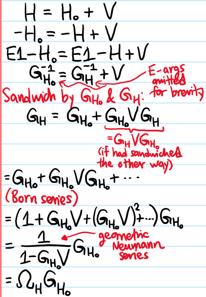
Problem: Starting from the decomposition \(H=H_0+V\), conclude that the resolvents \(G_H,G_{H_0}\) of \(H\) and \(H_0\) are related by:
\[G_H=\Omega_HG_{H_0}\]
where the Moller scattering operator \(\Omega_H\) of \(H\) depends on the choice of decomposition \(H=H_0+V\):
\[\Omega_H:=\frac{1}{1-G_{H_0}V}\]
Solution:
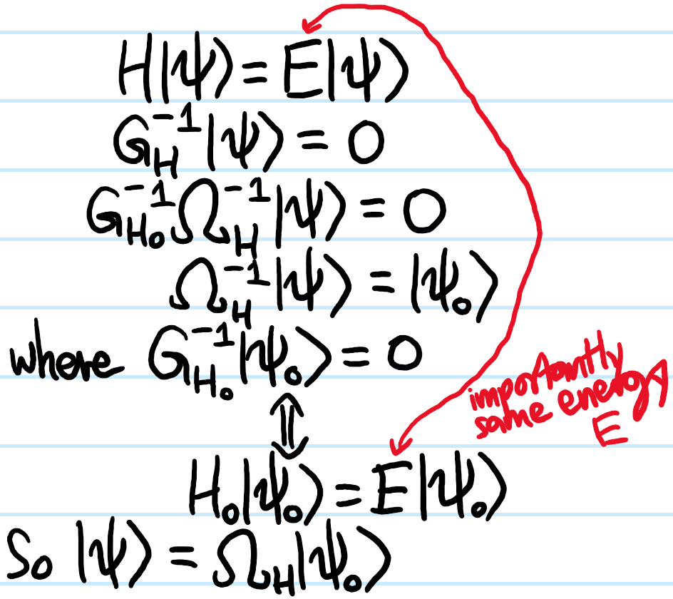
Problem: Starting from the Schrodinger equation \(H|\psi\rangle=E|\psi\rangle\) in the unusual form:
\[G^{-1}_H(E)|\psi\rangle=0\]
Use the result above to deduce the Lippman-Schwinger equation:
\[|\psi\rangle=\Omega_H|\psi_0\rangle\]
where \(H=H_0+V\) can be decomposed in any way one pleases, so long as this is reflected in the Moller scattering operator \(\Omega_H\) and the “free state” \(|\psi_0\rangle\) with commensurate energy \(H_0|\psi_0\rangle=E|\psi_0\rangle\) (thus, \(\Omega_H\) is “energy-conserving”).
Solution:
Problem: How is this form of the Lippman-Schwinger equation typically applied to quantum mechanical scattering?
Solution: The decomposition is chosen such that \(H_0=|\textbf P|^2/2\mu\) is a purely kinetic Hamiltonian and \(V\) is a corresponding \(2\)-body scattering potential for two particles of reduced mass \(\mu\) (working in the ZMF). In this case, one typically takes \(|\psi_0\rangle:=|\textbf k\rangle\) to be a plane wave \(H_0\)-eigenstate with energy \(E_{\textbf k}=\hbar^2|\textbf k|^2/2\mu\). Furthermore, one typically chooses the retarded Moller scattering operator \(\Omega_H^+(E_{\textbf k})=\frac{1}{1-G_{H_0}^+(E_{\textbf k})V}\) as an ad hoc way of cherrypicking the physical, outward-propagating solution \(|\psi\rangle:=|\psi^+_{\textbf k}\rangle\). Finally, it is convenient to work in a specific basis, typically the \(\textbf X\)-eigenbasis. Altogether then, the useful form of the Lippman-Schwinger equation for scattering theory is:
\[\psi_{\textbf k}^+(\textbf x)=\langle\textbf x|\Omega^+_H(E_{\textbf k})|\textbf k\rangle\]
To actually evaluate this, one ultimately has to unwrap the earlier geometric Neumann series for \(\Omega^+_H(E_{\textbf k})=1+G^+_{H_0}(E_{\textbf k})V+…\) and perhaps truncate at some partial sum to yield a Born approximation to \(\psi_{\textbf k}^+(\textbf x)\):
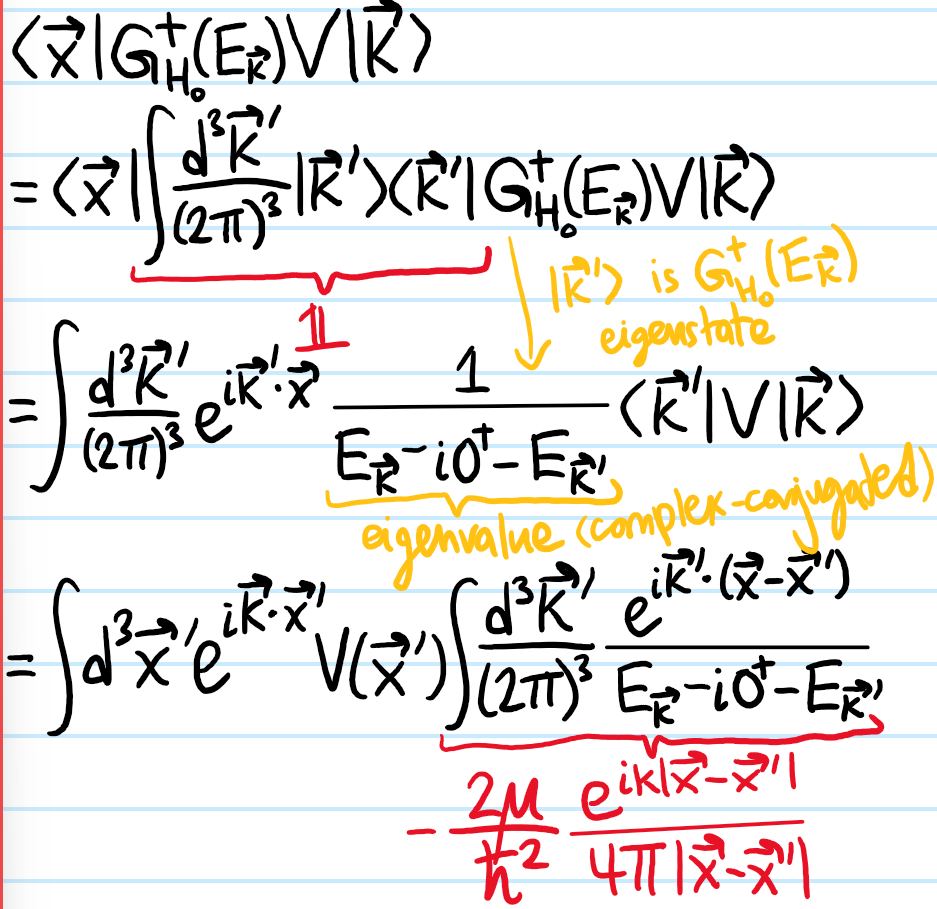
\[\psi_{\textbf k}^+(\textbf x)=e^{i\textbf k\cdot\textbf x}+\langle\textbf x|G^+_{H_0}(E_{\textbf k})V|\textbf k\rangle+…\]
Gauge-fixing the \(\textbf X\)-eigenstates to be an orthonormal basis in the sense that \(\langle\textbf x|\textbf x’\rangle=\delta^3(\textbf x-\textbf x’)\) and \(\int d^3\textbf x|\textbf x\rangle\langle\textbf x|=1\), and having implicitly assumed the normalization \(\langle\textbf x|\textbf k\rangle = e^{i\textbf k\cdot\textbf x}\), then one has \(\langle\textbf k|\textbf k’\rangle=(2\pi)^3\delta^3(\textbf k-\textbf k’)\) and \(\int\frac{d^3\textbf k}{(2\pi)^3}|\textbf k\rangle\langle\textbf k|=1\). Hence:
Problem: Is this perturbation theory?
Solution: It’s not really perturbation theory in the sense that the energies are just taken to be \(E=\hbar^2|\textbf k|^2/2m\), rather one is much more interested in the eigenstates (asymptotically especially!) from which other kinds of data like scattering amplitudes and cross sections, etc. are more interesting. So the goals of the \(2\) programs are different.
Problem: Consider some \(H_0\)-eigenstate \(|0\rangle\) with energy \(H_0|0\rangle=E_0|0\rangle\). Evaluate the expectation \(\langle 0|G_{H_0}(E)|0\rangle\). Hence, for \(H=H_0+V\), show that \(\langle 0|G_H(E)|0\rangle\) looks the same as \(\langle 0|G_{H_0}(E)|0\rangle\) except with \(E_0\mapsto E_0+\Sigma_H(E;|0\rangle)\) where the self-energy \(\Sigma_{|0\rangle,V}(E)\in\textbf C\) of the \(H_0\)-eigenstate \(|0\rangle\) due to the perturbation \(V\) is given by the usual:
\[\Sigma_{|0\rangle,V}(E)=V_{00}+\sum_{n\neq 0}V_{0n}\frac{1}{E-E_n}V_{n0}+\sum_{n,m\neq 0}V_{0n}\frac{1}{E-E_n}V_{nm}\frac{1}{E-E_m}V_{m0}+…\]
where \(V_{nm}:=\langle n|V|m\rangle\) are the matrix elements of the perturbation \(V\) in the unperturbed \(H_0\)-eigenbasis.
Problem: What are the interpretations of \(\Re\Sigma_{|0\rangle,V}(E)\) and \(\Im\Sigma_{|0\rangle,V}(E)\)?
Solution:
By tracking the movement of a simple pole \(E_n\) of \(G_H(E)\) in the complex \(E\)-plane, one can recover the eigenvalue and eigenstate corrections of perturbation theory.
Solution: Shine the spotlight on some eigenstate \(|n\rangle\) and its associated energy \(E_n\) by separating the unperturbed resolvent as:
\[G_{H_0}(E)=\frac{|n\rangle\langle n|}{E-E_n}+\sum_{m\neq n}\frac{|m\rangle\langle m|}{E-E_m}\]
and substitute it into the geometric series for \(G_H=G_H(E)\):
\[G_H=G_{H_0}+G_{H_0}VG_{H_0}+G_{H_0}VG_{H_0}VG_{H_0}+…\]
for instance:
\[G_{H_0}VG_{H_0}=\frac{|n\rangle\langle n|V|n\rangle\langle n|}{(E-E_n)^2}+\sum_{m\neq n}\frac{|n\rangle\langle n|V|m\rangle\langle m|+h.c.}{(E-E_n)(E-E_m)}+\sum_{m,\ell\neq n}\frac{|m\rangle\langle m|V|\ell\rangle\langle\ell|}{(E-E_m)(E-E_{\ell})}\]
The first term in the sum turns \(E=E_n\) from a simple pole into a double pole. It turns out this is what’s responsible for shifting the location of the pole away from \(E=E_n\), in other words, perturbing the eigenvalue. Meanwhile the series in the middle contributes to the residue at \(E=E_n\) because \(m\neq n\). Clearly they must be responsible for perturbing the eigenstate. Finally, because \(m,\ell\neq n\) in the last sum, it will be analytic in a neighbourhood of \(E=E_n\), in other words: crap.
Strictly speaking, after including the \(G_{H_0}VG_{H_0}\) term from the geometric Neumann-Born-Laurent series, the pole still sits at \(E=E_n\), just that its order has increased from \(1\to 2\). But consider as an example the geometric series \(1+1/x+1/x^2+…\). For any finite partial sum truncation, the pole sits at \(x=0\). But for \(|x|>1\) this converges absolutely to \(x/(x-1)\) where now the pole has been displaced to \(x=1\). Or just take any function like \(\tan(x)\) and Taylor expand it around \(x=0\) say; although all the terms in that Taylor series are analytic, the limiting behavior must be non-analytic at \(x=\pm\pi/2\). It’s basically a more extreme version of a phase transition, since singularities are more extreme than discontinuities.
Anyways, the fact that its the expectation \(\langle n|V|n\rangle\) which is sitting in the numerator of the double pole term means that this is the \(1^{\text{st}}\)-order correction to the energy. Similarly, decomposing into partial fractions:
\[\frac{1}{(E-E_n)(E-E_m)}=\frac{1}{E_n-E_m}\left(\frac{1}{E-E_n}-\frac{1}{E-E_m}\right)\]
only the first term \(\sim(E-E_n)^{-1}\) contributes to the residue at \(E=E_n\), and moreover this eigenstate contribution is just \(\sum_{m\neq n}\frac{\langle m|V|n\rangle}{E_n-E_m}|m\rangle\). Continuing to higher-order terms in the expansion reproduces the next formulas.
Problem #\(6\): Let \(H=H(\lambda)\) be a non-degenerate Hamiltonian depending on a parameter \(\lambda\) (not necessarily infinitesimal), and let \(|n\rangle=|n(\lambda)\rangle\) be a normalized \(H\)-eigenstate with energy \(E_n=E_n(\lambda)\). By differentiating the spectral equation:
\[H|n\rangle=E_n|n\rangle\]
with respect to \(\lambda\), prove the Hellman-Feynman theorems for the rate of change of the eigenvalue \(E_n\) and the \(H\)-eigenstate \(|n\rangle\):
\[\frac{\partial E_n}{\partial\lambda}=\biggr\langle n\biggr|\frac{\partial H}{\partial\lambda}\biggr|n\biggr\rangle\]
\[\frac{\partial|n\rangle}{\partial\lambda}=\sum_{m\neq n}\frac{\biggr\langle m\biggr|\frac{\partial H}{\partial\lambda}\biggr|n\biggr\rangle}{E_n-E_m}|m\rangle\]
(for the latter, one also has to fix the global \(U(1)\) gauge via \(\langle n|\frac{\partial|n\rangle}{\partial\lambda}\in\textbf R\)).
Solution #\(6\): The product rule gives:
\[\frac{\partial H}{\partial\lambda}|n\rangle+H\frac{\partial|n\rangle}{\partial\lambda}=\frac{\partial E_n}{\partial\lambda}|n\rangle+E_n\frac{\partial |n\rangle}{\partial\lambda}\]
This is like having \(2\) vectors \((a,b,c)=(d,e,f)\); naturally one’s instinct would be to equate components \(a=d,b=e,c=f\). In this context, what that looks like is projecting both sides onto an arbitrary \(H\)-eigenstate \(|m\rangle\) to equate the scalar components of all vectors:
\[\biggr\langle m\biggr|\frac{\partial H}{\partial\lambda}\biggr|n\biggr\rangle+E_m\langle m|\frac{\partial|n\rangle}{\partial\lambda}=\frac{\partial E_n}{\partial\lambda}\delta_{nm}+E_n\langle m|\frac{\partial|n\rangle}{\partial\lambda}\]
the Hellman-Feynman theorems then arise by considering the \(2\) cases \(m=n\) and \(m\neq n\). There is a priori also a component of the rate of change \(\partial|n\rangle/\partial\lambda\) of the \(H\)-eigenstate \(|n\rangle\) along itself with amplitude \(\langle n|\frac{\partial|n\rangle}{\partial\lambda}\), but due to normalization \(\langle n|n\rangle=1\Rightarrow\frac{\partial\langle n|}{\partial\lambda}|n\rangle+\langle n|\frac{\partial|n\rangle}{\partial\lambda}=0\Rightarrow\Re\langle n|\frac{\partial|n\rangle}{\partial\lambda}=0\Rightarrow\langle n|\frac{\partial|n\rangle}{\partial\lambda}=0\); this is like saying that an ant crawling on a sphere \(|\textbf x|^2=\text{const}\) must have orthogonal position and velocity \(\textbf x\cdot\dot{\textbf x}=0\).
The Hellman-Feynman theorems are reminiscent of formulas such as:
\[i\hbar\frac{d}{dt}\langle\phi|A|\psi\rangle=\langle\phi|[A,H]|\psi\rangle+i\hbar\biggr\langle\phi\biggr|\frac{\partial H}{\partial t}\biggr|\psi\biggr\rangle\]
in which one takes \(A=H\) and \(\lambda=t\), as well as the special case \(\phi=\psi\) of Ehrenfest’s theorem.
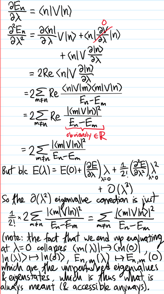
Problem #\(7\): Hence, by applying the Hellman-Feynman theorems to a linearly perturbed Hamiltonian \(H=H_0+\lambda V\), deduce the \(O(\lambda^2)\) corrections to both the eigenvalues \(E_n\) and eigenstates \(|n\rangle\) of the unperturbed Hamiltonian \(H_0\) in the presence of a perturbation \(V\).
Solution #\(7\): Specialized to the case of this particular linearly perturbed Hamiltonian, one has trivially \(\frac{\partial H}{\partial\lambda}=V\). With this in mind, one simply takes the Hellman-Feynman formulas and differentiate them again with respect to \(\lambda\):
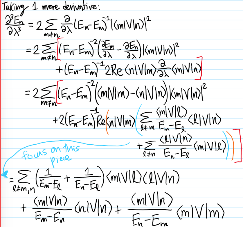
For fun, here is a (failed!) attempt to compute the \(O(\lambda^3)\) eigenvalue correction (what’s the mistake?):

And for the \(O(\lambda^2)\) eigenstate correction, refer to this document.
TO DO: extend/generalize all the above discussion to degenerate and time dependent perturbation theory! Also find where to put the following snippets:
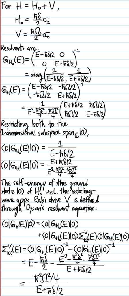
Problem: In the rotating frame of a Rabi drive \((\omega,\Omega)\) detuned by a small amount \(\delta:=\omega-\omega_0\) from a bare resonance, within the rotating wave approximation one has \(H=H_0+V\) with \(H_0=\frac{\hbar\delta}{2}\sigma_z\) and \(V=\frac{\hbar\Omega}{2}\sigma_x\). Evaluate the self-energy \(\Sigma^V_{|0\rangle}(E)\) in the one-dimensional subspace spanned by the ground state \(|0\rangle\), and show that it reproduces the \(2^{nd}\)-order AC Stark shift when evaluated on-shell (i.e. for \(E=-\hbar\delta/2\)).
Solution: