
A qubit is any quantum system with a two-dimensional state space \(\mathcal H\cong\textbf C^2\). In particular because the state space is two-dimensional \(\dim\textbf C^2=2\), the Gram-Schmidt orthogonalization algorithm guarantees the existence of an orthonormal basis \(|0\rangle,|1\rangle\in\mathcal H\) of state vectors spanning \(\text{span}_{\textbf C}|0\rangle,|1\rangle=\mathcal H\) the entire state space \(\mathcal H\) of the qubit. For a larger system of \(N\in\textbf Z^+\) qubits, the corresponding state space \(\mathcal H_N\) is the \(N\)-fold tensor product \(\mathcal H_N\cong\left(\textbf C^2\right)^{\otimes N}\cong\textbf C^{2^N}\) of each qubit’s individual two-dimensional state space, with the dimension \(\dim\mathcal H_N\) of this composite Hilbert space \(\mathcal H_N\) growing exponentially \(\dim\mathcal H_N=2^N\) in the number \(N\) of qubits.
Bloch Sphere Representation of Physical Qubit States
One useful way to visualize physical qubit states \(|\psi\rangle\in P(\textbf C^2)\) (of an individual qubit) is via the Bloch sphere. The idea is to think of the qubit as being concretely realized by the spin angular momentum degree of freedom of a spin \(s=1/2\) isolated electron \(e^-\) whose position is fixed in an inertial frame in \(\textbf R^3\). Suppose one were to then make a measurement (e.g. with a suitable Stern-Gerlach filter) of the electron’s spin angular momentum \(\textbf S\) along some arbitrary direction \(\hat{\textbf n}\in S^2\) of one’s liking given in spherical coordinates by \(\hat{\textbf n}=\cos\phi\sin\theta\hat{\textbf i}+\sin\phi\sin\theta\hat{\textbf j}+\cos\theta\hat{\textbf k}\). Then for spin \(s=1/2\) quantum particles, there are precisely two possible (though not necessarily equiprobable) outcomes of such a measurement, namely \(m_s=\pm 1/2\) corresponding to an electron \(e^-\) either “spinning” aligned or anti-aligned with the direction \(\hat{\textbf n}\) of measurement. In particular, the electron’s spin state then collapses non-unitarily to the corresponding \(\hat{\textbf n}\cdot\textbf S\)-eigenstate which one can check are given by \(|m_s=1/2\rangle=\cos(\theta/2)|0\rangle+e^{i\phi}\sin(\theta/2)|1\rangle\) and \(|m_s=-1/2\rangle=-e^{-i\phi}\sin(\theta/2)|0\rangle+\cos(\theta/2)|1\rangle\) where \(|0\rangle,|1\rangle\) is the \(S_3\)-eigenbasis. In particular, the \(\hat{\textbf n}\)-aligned spin angular momentum eigenstate \(|m_s=1/2\rangle\) of \(\hat{\textbf n}\cdot\textbf S\) provides a general parameterization of an arbitrary electron spin state in \(\textbf C^2\) simply because the electron \(e^-\) has to be “spinning” along some direction \(\hat{\textbf n}\in S^2\) at all times (of course the same is true of the \(\hat{\textbf n}\)-antialigned spin angular momentum eigenstate \(|m_s=-1/2\rangle\), but it’s just more intuitive to work with the former). The map \(|m_s=1/2\rangle\mapsto\hat{\textbf n}\) is then the essence of the Bloch sphere \(S^2\) representation of physical qubit states.
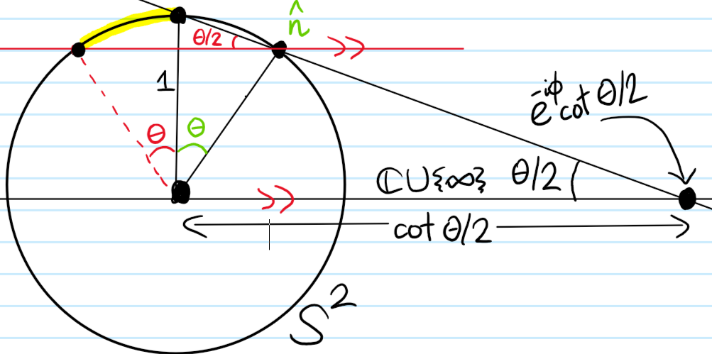
As an aside, there is another nice way to visualize the Bloch mapping \(|m_s=1/2\rangle\mapsto\hat{\textbf n}\), which is a map from \(\textbf C^2\to S^2\). The idea is to decompose it as the composition of a Hopf fibration \(\textbf C^2\to\textbf C\cup\{\infty\}\) onto the extended complex plane \(\textbf C\cup\{\infty\}\), followed by an (inverse) stereographic projection onto an equatorial Riemann sphere \(\textbf C\cup\{\infty\}\to S^2\). Specifically, the Hopf fibration exploits the projective nature of \(P(\textbf C^2)\) by computing the ratio of probability amplitudes \(|\psi\rangle\mapsto\frac{\langle 0|\psi\rangle}{\langle 1|\psi\rangle}\) so in particular \(\cos(\theta/2)|0\rangle+e^{i\phi}\sin(\theta/2)|1\rangle\mapsto e^{-i\phi}\cot(\theta/2)\), and the rest is summarized in this picture:
This discussion has been implicitly focused on the pure quantum states of the qubit, although one could also allow more general mixed ensembles of pure states described by a density operator \(\rho\). In that case, it turns out points inside the Bloch sphere (called the Bloch ball \(|\hat{\textbf n}|<1\)) correspond precisely to such mixed ensembles.
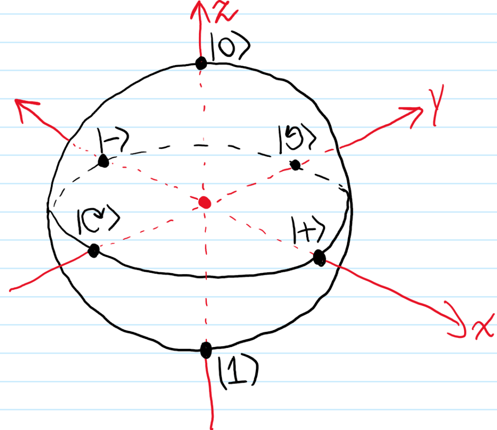
where one can clearly see by setting \(\theta=\pi/2\) in the formula and \(\phi=0,\pi/2,\pi,3\pi/2\) that those cardinal points on the Bloch sphere correspond to the physical qubit states \(|+\rangle=\frac{1}{\sqrt 2}|0\rangle+\frac{1}{\sqrt 2}|1\rangle\), \(|-\rangle=\frac{1}{\sqrt 2}|0\rangle-\frac{1}{\sqrt 2}|1\rangle)\), \(|⟲\rangle=\frac{1}{\sqrt 2}|0\rangle+\frac{i}{\sqrt 2}|1\rangle\), and \(|⟳\rangle=\frac{1}{\sqrt 2}|0\rangle-\frac{i}{\sqrt 2}|1\rangle\) (here, the swirly-arrow notation ⟲,⟳ is actually more of a nod to thinking of the qubit states as photon \(\gamma\) polarization states, specifically as circularly polarized light).
“Qubit Strings” and Quantum Logic Gates
Given a classical bit string \(\xi=b_1b_2b_3…b_N\in\{0,1\}^N\) of length \(|\xi|=N\), the “qubit string” analog of it is given by the obvious isomorphism \(\{0,1\}^N\to\mathcal H_N\) into the state space \(\mathcal H_N\) of an \(N\)-qubit system defined by \(b_1b_2b_3…b_N\mapsto|b_1\rangle\otimes|b_2\rangle\otimes|b_3\rangle\otimes…\otimes|b_N\rangle\). Since there are of course \(2^N\) bit strings \(\xi\in\{0,1\}^N\) of length \(N\), this is indeed an isomorphism with its image defining the canonical unentangled basis \(\text{span}_{\textbf C}\left\{\otimes_{i=1}^N|b_i\rangle:b_i=0\text{ or }1\text{ for all }1\leq i\leq N\right\}=\mathcal H_N\) for \(\mathcal H_N\). In practice, it will often be convenient for “side quantum computations” to “pad” several additional qubits whose states are all initialized “spin-up” \(|0\rangle\) on the Bloch sphere, thus \(|b_1\rangle\otimes|b_2\rangle\otimes|b_3\rangle\otimes…\otimes|b_N\rangle\mapsto |b_1\rangle\otimes|b_2\rangle\otimes|b_3\rangle\otimes…\otimes|b_N\rangle\otimes|0\rangle\otimes|0\rangle\otimes…\otimes|0\rangle\).
Recall that in the circuit model \(\mathcal M_{\text{circuit}}\) of classical computation, the computational steps \(\Gamma_i:\{0,1\}^*\to\{0,1\}^*\) that might comprise a classical algorithm for computing some function \(f:\{0,1\}^*\to\{0,1\}^*\) were a universal set of logic gates like \(\text{AND},\text{OR},\text{NOT}\), etc. Earlier, we just saw that quantumly, we should replace \(N\)-bit strings by their analogous \(N\)-qubit states. What becomes the analog of the logic gates that form the backbone of classical computation in the circuit model? Well, now we just promote them to quantum logic gates acting on multi-qubit states in what should now be thought of as the circuit model of quantum computation. More precisely, an \(N\)-qubit quantum logic gate is any unitary operator in \(U\left(\textbf C^{2^N}\right)\) acting on \(N\)-qubit states.
For \(N=1\) qubit, continuing with the earlier example of a qubit realized via the spin angular momentum degree of freedom \(\textbf S\) of an electron \(e^-\), any unitary operator in \(U(\textbf C^2)\) must look like an intrinsic rotation \(e^{-i\Delta{\boldsymbol{\phi}}\cdot\textbf S/\hbar}\in U(\textbf C^2)\) of the electron \(e^-\) (which includes its “spin” axis \(\hat{\textbf n}\)) by an angular displacement \(\Delta{\boldsymbol{\phi}}\in\textbf R^3\). More precisely, for spin \(s=1/2\) quantum particles, we have \([\textbf S]_{|0\rangle,|1\rangle}^{|0\rangle,|1\rangle}=\frac{\hbar}{2}\boldsymbol{\sigma}\), so in the \(S_3\)-eigenbasis \(|0\rangle,|1\rangle\) we have the \(SU(2)\)-analog of Euler’s formula:
\[\left[e^{-i\Delta{\boldsymbol{\phi}}\cdot\textbf S/\hbar}\right]_{|0\rangle,|1\rangle}^{|0\rangle,|1\rangle}=e^{-i\Delta{\boldsymbol{\phi}}\cdot\boldsymbol{\sigma}/2}=\cos\left(\frac{\Delta\phi}{2}\right)1-i\sin\left(\frac{\Delta\phi}{2}\right)(\Delta\hat{\boldsymbol{\phi}}\cdot\boldsymbol{\sigma})\]
where \(\Delta{\boldsymbol{\phi}}=\Delta{\phi}\Delta\hat{\boldsymbol{\phi}}\). In particular, we have the following standard single-qubit quantum logic gates:

where as a special case of Euler’s \(SU(2)\)-formula we have for \(j=0,1,2,3\) that \(\sigma_j=ie^{-i\pi\sigma_j/2}\). However, the \(i\) in front is merely a global \(U(1)\) phase factor which is explicitly ignored in the Bloch \(S^2\) representation of physical qubit states. This is why it is accurate to think of both the Pauli and Hadamard quantum logic gates as encoding \(180^{\circ}=\pi\text{ rad}\) rotations of the qubit state on the Bloch sphere about different axes. Note of course that the Pauli gates are exactly identical to the usual \(\frak{su}\)\((2)\) Pauli matrices. In particular, the Pauli \(X\)-gate is the quantum analog of the classical \(\text{NOT}\) logic gate since when acting on the \(S_3\)-eigenbasis it swaps \(|0\rangle\leftrightarrow|1\rangle\) (of course \(X\) also acts on arbitrary \(\textbf C^2\) superpositions of \(|0\rangle\) and \(|1\rangle\) too on the Bloch \(S^2\) which is the novelty of quantum computing!). And the phase shift gate \(P_{\Delta\phi}\) is really a one-parameter subgroup of quantum logic gates parameterized by the azimuth \(\Delta\phi\in\textbf R\), for instance \(P_{\Delta\phi=\pi}=Z\) and one sometimes also sees the quantum logic gates \(S=P_{\Delta\phi=\pi/2}\) and \(T=P_{\Delta\phi=\pi/4}\). Note that a lot of this notation does clash with standard quantum mechanics notation on \(\textbf R^3\) where \(X,Y,Z\) are often used to denote the Cartesian components of the position observable \(\textbf X\) (although this is partially amended by the existence of the alternative notation \(X_1,X_2,X_3\)). However, an irreparable notational conflict lies in the Hadamard gate \(H=(X+Z)/\sqrt{2}\) where \(H\) is conventionally reserved for the Hamiltonian of a quantum system. For each of these quantum logic gates, there exists a corresponding circuit schematic symbol which (usually) consists simply of enclosing the letter of the gate into a rectangular box and adding an appropriate number of input and output qubit feeds, for example the Hadamard gate:

Just as the classical \(\text{AND}\) and \(\text{OR}\) logic gates accept input bit strings \(\xi\in\{0,1\}^2\) of length \(|\xi|=2\), so there are also two-qubit quantum logic gates in \(U(\textbf C^2\otimes\textbf C^2)\). Here we list a few standard ones:
- CX Gate: just as the Pauli \(X\)-gate can be thought of as a quantum NOT gate, the CX gate (called the controlled NOT gate) is a controlled version of the Pauli \(X\)-gate. More precisely, when acting on the unentangled \(2\)-qubit basis \(|0\rangle\otimes|0\rangle, |0\rangle\otimes|1\rangle, |1\rangle\otimes|0\rangle, |1\rangle\otimes|1\rangle\) (also called “the” computational basis for \(2\)-qubit systems), the input state \(|b_1\rangle\) of a control qubit is acted upon by the identity \(1\) (i.e. nothing happens to it) whereas the input state \(|b_2\rangle\) of a second target qubit may or may not be acted upon by the Pauli \(X\)-gate \(|b_2\rangle\mapsto X|b_2\rangle\) depending on the control qubit’s input state \(|b_1\rangle\). Such a “truth table” can be expressed as \(CX|b_1\rangle\otimes|b_2\rangle:=|b_1\rangle\otimes X^{b_1}|b_2\rangle=|b_1\rangle\otimes|b_1\text{ XOR } b_2\rangle\) for \(b_1,b_2\in\{0,1\}\), thus showing that the controlled NOT gate \(CX\) can also be viewed as a sort of quantum analog of the classical exclusive or (XOR) logic gate. Note that the action of the controlled NOT gate \(CX\) on arbitrary states in \(\textbf C^{2}\otimes\textbf C^2\) follows from the above truth table by linearity. The controlled NOT gate \(CX\) thus also has matrix representation:
\[[CX]_{|0\rangle\otimes|0\rangle, |0\rangle\otimes|1\rangle, |1\rangle\otimes|0\rangle, |1\rangle\otimes|1\rangle}^{|0\rangle\otimes|0\rangle, |0\rangle\otimes|1\rangle, |1\rangle\otimes|0\rangle, |1\rangle\otimes|1\rangle}=\text{diag}(1_{2\times 2},[X]_{|0\rangle,|1\rangle}^{|0\rangle,|1\rangle})=\begin{pmatrix}1&0&0&0\\0&1&0&0\\0&0&0&1\\0&0&1&0\end{pmatrix}\]
Viewed as a rotation on some kind of entangled Bloch sphere, one also has \(CX=e^{\pm i\frac{\pi}{4}(1-Z_1)\otimes(1-X_2)}\); this can be checked by a direct computation but I still don’t feel I have a strong intuition for why this is right, in particular why it should involve the Pauli \(Z\)-gate of the control qubit?
- CY Gate: The controlled Pauli \(Y\)-gate is conceptually identical to the definition of the controlled NOT gate (also called the controlled Pauli \(X\)-gate) just with \(X\mapsto Y\) everywhere in the discussion. The upshot is that \(CY|b_1\rangle\otimes|b_2\rangle=|b_1\rangle\otimes Y^{b_1}|b_2\rangle\) or equivalently:
\[[CY]_{|0\rangle\otimes|0\rangle, |0\rangle\otimes|1\rangle, |1\rangle\otimes|0\rangle, |1\rangle\otimes|1\rangle}^{|0\rangle\otimes|0\rangle, |0\rangle\otimes|1\rangle, |1\rangle\otimes|0\rangle, |1\rangle\otimes|1\rangle}=\text{diag}(1_{2\times 2},[Y]_{|0\rangle,|1\rangle}^{|0\rangle,|1\rangle})=\begin{pmatrix}1&0&0&0\\0&1&0&0\\0&0&0&-i\\0&0&i&0\end{pmatrix}\]
The controlled Pauli \(Y\)-gate also has a Bloch sphere representation.
- CZ Gate: The controlled Pauli \(Z\)-gate is again the same idea (i.e. the idea of having a control qubit to control whether or not a target qubit is acted on by the Pauli \(Z\)-gate), i.e. \(CZ|b_1\rangle\otimes|b_2\rangle=|b_1\rangle\otimes Z^{b_1}|b_2\rangle\) or:
\[[CZ]_{|0\rangle\otimes|0\rangle, |0\rangle\otimes|1\rangle, |1\rangle\otimes|0\rangle, |1\rangle\otimes|1\rangle}^{|0\rangle\otimes|0\rangle, |0\rangle\otimes|1\rangle, |1\rangle\otimes|0\rangle, |1\rangle\otimes|1\rangle}=\text{diag}(1_{2\times 2},[Z]_{|0\rangle,|1\rangle}^{|0\rangle,|1\rangle})=\begin{pmatrix}1&0&0&0\\0&1&0&0\\0&0&1&0\\0&0&0&-1\end{pmatrix}\]
The controlled Pauli \(Z\)-gate also has a Bloch sphere representation.
Measurement
Recall that in quantum mechanics, given an observable \(\textbf X\) (e.g. position) with spectrum \(\textbf x_1,\textbf x_2,…\) and a quantum system in some arbitrary state \(|\psi\rangle\), the Born rule asserts that each \(\textbf x_j\) has probability \(|\langle\textbf x_j|\psi\rangle|^2\) of being the outcome of an \(\textbf X\)-measurement. Specific to the Copenhagen interpretation of quantum measurement is that the state \(|\psi\rangle\) also collapses \(|\psi\rangle\mapsto|\textbf x_j\rangle\) to the \(\textbf X\)-eigenstate \(|\textbf x_j\rangle\) associated to the measured value \(\textbf x_j\). In other words, the measurement of the state \(|\psi\rangle\) randomly projects \(|\psi\rangle\) onto one of the eigenstates of \(\textbf X=\textbf x_1|\textbf x_1\rangle\langle\textbf x_1|+\textbf x_2|\textbf x_2\rangle\langle \textbf x_2|+…\) (this is \(|\psi\rangle\mapsto|\textbf x_j\rangle\langle\textbf x_j|\psi\rangle\cong|\textbf x_j\rangle\)) . However, regardless of the outcome, this measurement process is non-unitary \(\notin U(\mathcal H)\) because a projection \(P^2=P\Rightarrow\det P=0\), being irreversible/non-invertible, must be non-unitary (with the \(\det P=1\) exception that if a quantum system already happens to be in some \(\textbf X\)-eigenstate \(|\textbf x_j\rangle\), then in that case an \(\textbf X\)-measurement simply collapses the state via the identity \(|\textbf x_j\rangle\mapsto|\textbf x_j\rangle\) which is trivially unitary). Another way to convince yourself why measurement is non-unitary is that the inner products \(\langle\psi_1|\psi_2\rangle\mapsto\langle \textbf x_1|\textbf x_2\rangle=\delta_{\textbf x_1,\textbf x_2}\) are not necessarily \(1\) after the measurement (the particular pair of states only has probability \(\text{Tr}()=\sum_{\textbf x\in\Lambda_{\textbf X}}|\langle\textbf x|\psi_1\rangle|^2|\langle\textbf x|\psi_2\rangle|^2\) of being unitary in this sense, assuming they’re unentangled).
Despite being non-unitary, whereas we defined quantum logic gates to be unitary, nothing says we can’t still exploit measurements to our advantage in quantum computation so that in a way they sort of are like just another kind of quantum logic gate (albeit non-unitary and non-deterministic). More precisely, since the measurement will essentially give some concrete bit string, it is common to perform classical computations with the results of measurements; however, note that this doesn’t actually add any novel computational power to quantum computing.
In analogy to the notion of a universal set of logic gates in the circuit model of classical computation, one has the notion of an approximately universal set of quantum logic gates; we want to only consider some finite collection of quantum logic gates as somehow “generating” via compositions all possible quantum logic gates in \(\bigcup_{N\in\textbf N}U\left(\textbf C^{2^N}\right)\), but the group \(\bigcup_{N\in\textbf N}U\left(\textbf C^{2^N}\right)\) has uncountably infinite order whereas any finite collection of quantum logic gates in \(\bigcup_{N\in\textbf N}U\left(\textbf C^{2^N}\right)\) clearly can only generate a countably infinite subgroup (this is similar to how the cyclic subgroup \(C_{\infty}=\{R^n:n\in\textbf N\}\) of \(SO(2)\) generated by some rotation matrix \(R\in SO(2)\) does not actually generate \(SO(2)\) itself, i.e. \(C_{\infty}\neq SO(2)\) again on order grounds \(|C_{\infty}|=\aleph_0<|SO(2)|\) though \(C_{\infty}\) will be dense in \(SO(2)\) provided the generator \(R=\begin{pmatrix}\cos\theta&-\sin\theta\\\sin\theta&\cos\theta\end{pmatrix}\) rotates \(\textbf R^2\) through an irrational angle \(\theta\in\textbf R-\textbf Q\)).
Definition (Approximate Universality): A collection of quantum logic gates \(\mathcal G\subseteq\bigcup_{N\in\textbf N}U\left(\textbf C^{2^N}\right)\) is said to be approximately universal iff for arbitrarily small \(\varepsilon>0\) and any quantum logic gate \(\Gamma\in\bigcup_{N\in\textbf N}U\left(\textbf C^{2^N}\right)\), there exists some quantum logic circuit \(\Gamma_1\circ\Gamma_2\circ…\) with each \(\Gamma_i\in\mathcal G\) such that \(|\Gamma-\Gamma_1\circ\Gamma_2\circ…|<\varepsilon\) in the operator norm, or equivalently \(\sup_{\langle\psi|\psi\rangle=1}|\Gamma|\psi\rangle-\Gamma_1\circ\Gamma_2\circ…|\psi\rangle|<\varepsilon\).
For instance, it can be checked that the collections \(\{\text{CX}\}\cup U(\textbf C^2)\) and \(\{CX,H,T\}\) are approximately universal sets of quantum logic gates. In fact, the former, being uncountably infinite, is actually an exactly universal set of quantum logic gates which means what it sounds like (i.e. \(\varepsilon=0\)).
Mechanical Model of Measurement
I wonder if one can build a mechanical model to illustrate this, e.g. a flashlight mounted on a spinner for an \(\textbf S\)-measurement of a qubit.
Quantum Complexity Classes
Recall that \(\textbf{BPP}\), called the bounded error probabilistic polynomial time complexity class, is the classical complexity class of all decision problems (or equivalently their binary languages \(\mathcal L\subseteq\{0,1\}^*\)) for which there exists a randomized polynomial-time algorithm with “better-than-random” probability of correctly computing the indicator function \(\in_{\mathcal L}:\{0,1\}^*\to\{0,1\}\) on each input bit string \(\xi\in\{0,1\}^*\). The quantum complexity class analog of the classical \(\textbf{BPP}\) complexity class is called \(\textbf{BQP}\), standing for bounded error quantum polynomial time, representing the set of all decision problems for which there exists a polynomial-time quantum circuit/algorithm using some particular approximately universal collection of quantum logic gates that correctly computes the answer to the decision problem at least \(2/3\) of the time (again, the \(2/3\) is sort of arbitrary).
One can check that \(\textbf{BQP}\) is independent of which particular collection of approximately universal quantum logic gates one uses. Just as classically, we have the quantum analog of Cobham’s thesis that \(\textbf{BQP}\) is the class of all “feasible quantum decision problems”. Indeed, there is a simple connection known between \(\textbf{BPP}\) and \(\textbf{BQP}\), namely that \(\textbf{BPP}\subseteq\textbf{BQP}\). The question of whether or not quantum computing is strictly more powerful than classical computing can be phrased roughly as the question: “is \(\textbf{BPP}=\textbf{BQP}\)”? If true, this would mean the answer is “no”.