Reciprocal Space

Problem: What is a lattice $\Lambda$? What does it mean to say that a lattice is Bravais? Give an example of a Bravais lattice and a non-Bravais lattice.

Solution: A lattice $\Lambda$ is any periodic set of lattice points in $\textbf R^d$ for some dimension $d$ (usually $d=2$ or $d=3$). More precisely, a lattice is said to be Bravais iff either of the following $2$ (logically equivalent) statements are true:

i) There exist $d$ linearly independent vectors $\textbf x_1,\textbf x_2,…,\textbf x_d\in\textbf R^d$ such that $\Lambda=\text{span}_{\textbf Z}(\textbf x_1,\textbf x_2,…,\textbf x_d)$ (aside: of course such a $\textbf Z$-basis certainly need not be unique).

ii) Begin at any lattice point $\textbf x\in\Lambda$, then close one’s eyes and walk to any other lattice point $\textbf x’\in\Lambda$ without turning one’s head. After opening one’s eyes, it looks as if one hasn’t moved at all (i.e. as if $\textbf x’=\textbf x$ even though that need not be true)!

An example of a $2$D Bravais lattice is the triangular lattice which is $\textbf Z$-spanned by the vectors $\textbf x_1=a\hat{\textbf x}$ and $\textbf x_2=\frac{\sqrt{3}}{2}\hat{\textbf x}+\frac{1}{2}\hat{\textbf y}$. An example of a $2$D lattice which is non-Bravais (but still a legitimate lattice) is a hexagonal honeycomb lattice.

Problem: Given a Bravais lattice $\Lambda$ and a volume $V\subseteq\textbf R^d$, what does it mean to say that $V$ is a unit cell of $\Lambda$? What does it mean if such a unit cell is primitive? What does it mean if such a unit cell is conventional? Give an example of a Bravais lattice $\Lambda$ and unit cell thereof which is conventional but non-primitive.

Solution: $V$ is said to be a unit cell of $\Lambda$ iff arbitrary $\Lambda$-translations tessellate the whole space $\textbf R^d$, i.e.

\[\bigcup_{\textbf x\in\Lambda} V+\textbf x=\textbf R^d\]

(in particular, a corollary of this definition is that $V$ is a unit cell of $\Lambda$ iff $V+\Delta\textbf x$ is a unit cell of $\Lambda$ for all $\Delta\textbf x\in\textbf R^d$ so the exact “location” of $V$ is irrelevant, only its shape matters).

A unit cell $V$ is said to be primitive iff it contains a single lattice point of $\Lambda$. Loosely speaking, this means $\#(V\cap\Lambda)=1$. More precisely, the volume $|V|$ of $V$ should coincide with the (positive) volume $|\det(\textbf x_1,\textbf x_2,…,\textbf x_d)|$ of the parallelepiped formed from an arbitrary $\textbf Z$-basis $\textbf x_1,\textbf x_2,…,\textbf x_d$ for $\Lambda$:

\[|V|=|\det(\textbf x_1,\textbf x_2,…,\textbf x_d)|\]

(aside: it is intuitively clear, and not hard to show, that because of the presence of the integer field $\textbf Z$, although the $\textbf Z$-basis itself is not unique, the (positive) volume $|\det(\textbf x_1,\textbf x_2,…,\textbf x_d)|$ is invariant with respect to all possible choices).

A unit cell $V$ for $\Lambda$ is said to be conventional iff some crystallographer arbitrarily decided they like that particular unit cell for $\Lambda$. Usually this is motivated by the unit cell being simpler to conceptualize than a primitive unit cell, or because it is more faithful representation of the symmetries of $\Lambda$.

For example, for a face-centered cubic Bravais lattice:

\[\Lambda_{\text{fcc}}=\text{span}_{\textbf Z}\left(\frac{a}{2}\hat{\textbf x}+\frac{a}{2}\hat{\textbf y},\frac{a}{2}\hat{\textbf x}+\frac{a}{2}\hat{\textbf z},\frac{a}{2}\hat{\textbf y}+\frac{a}{2}\hat{\textbf z}\right)\]

(aside: the basis vectors $\textbf x_i$ for $i=1,…,d$ are also called primitive lattice vectors or primitive translation vectors, the word “primitive” being a reference to the fact that one possible unit cell for any Bravais lattice $\Lambda$ is always the parallelepiped $V$ formed by the $\textbf x_i$ which trivially has $|V|=|\det\{\textbf x_i\}|$ and so is primitive).

Although the $\textbf x$-notation here is suggestive of the Bravais lattice $\Lambda$ residing in real space $\textbf R^d$, in fact all the discussion hitherto also applies to reciprocal space.

Problem: Define the reciprocal Bravais lattice $\Lambda^*$ associated to a given real space Bravais lattice $\Lambda$.

Solution: There are several logically equivalent formulations:

i) \[\textbf k\in\Lambda^*\Leftrightarrow\textbf k\cdot\textbf x\equiv 0\pmod 2\pi\] for all $\textbf x\in\Lambda$.

ii) If $(\textbf x_1,…,\textbf x_d)$ is any $\textbf Z$-basis for $\Lambda$, then any set of vectors $\textbf k_1,…,\textbf k_d$ obeying $\textbf k_i\cdot\textbf x_j=2\pi\delta_{ij}$ will $\textbf Z$-span $\Lambda^*$:

\[\Lambda^*=\text{span}_{\textbf Z}(\textbf k_1,…,\textbf k_d)\]

(for $d=3$ only, one has the explicit formulas:

\[\textbf k_1=2\pi\frac{\textbf x_2\times\textbf x_3}{V}\]

\[\textbf k_2=2\pi\frac{\textbf x_2\times\textbf x_3}{V}\]

\[\textbf k_3=2\pi\frac{\textbf x_1\times\textbf x_2}{V}\]

where $V:=\textbf x_1\cdot(\textbf x_2\times\textbf x_3)$ is the primitive unit cell volume in real space.

iii) If $\Lambda$ is associated to the Dirac comb $\sum_{\textbf x’\in\Lambda}\delta^d(\textbf x-\textbf x’)$, then the Fourier transform of $\Lambda$ is the Dirac comb $\sum_{\textbf k’\in\Lambda}\delta^d(\textbf k-\textbf k’)$ which may be associated to the reciprocal lattice $\Lambda^*$ itself (thus, x-ray crystallography (in the Fraunhofer limit) is simply the art of photographing reciprocal space!). More generally, for any $\Lambda$-periodic function $\psi(\textbf x)$, the Fourier transform $\psi(\textbf k):=\int\frac{d^d\textbf k}{(2\pi)^d}e^{-i\textbf k\cdot\textbf x}\psi(\textbf x)$ is given by:

\[\]

Introduce the Wigner-Seitz primitive unit cell of a Bravais lattice; in reciprocal space called the Brillouin zone of $\Lambda^*$, perpendicular bisector construction.

Problem: Although the Bravais lattices $\Lambda$ considered so far have been, strictly speaking, infinite in extent, in practice all solids are finite in size, containing a finite number $|\Lambda|<\infty$ of lattice points. Given this consideration, how many quantum $\textbf k$-states are available in each Brillouin zone (in the extended zone scheme; equivalently, in the reduced zone scheme this would be phrased as a question of how many $\textbf k$-states are available in each band).

In $\textbf R^3$, there is a standard classification of 3D Bravais lattices into $14$ disjoint buckets based on how symmetric the conventional unit cell is (most symmetric is the primitive cubic 3D Bravais lattice, most asymmetric is the primitive triclinic 3D Bravais lattice, all the other 3D Bravais lattices lie on a spectrum somewhere in between).
A crystal $\Gamma$ is the convolution of a 3D Bravais lattice $\Lambda$ with a motif $M$ of atoms or molecules: $\Gamma=\Lambda*M$.
A lattice plane is any 2D affine subspace of the crystal $\Gamma$, denoted by Miller indices $(hkl)$ where the reciprocal lattice vector $h\textbf a^*+k\textbf b^*+l\textbf c^*$ is the normal vector the lattice plane. In other words, this yields the Weiss zone law $(U\textbf a+V\textbf b+W\textbf c)\cdot(h\textbf a^*+k\textbf b^*+l\textbf c^*)=hU+kV+lW=0$.
The multiplicity of a lattice plane $(hkl)$ is $|\{hkl\}|$ and is at most $|\{hkl\}|\leq 2^3\times 3!=48$.
There are $2$ distinct solutions to achieving close packing of identical spheres in $\textbf R^3$ (i.e. saturating the maximum packing efficiency of $\eta=\frac{\pi}{3\sqrt{2}}\approx 74\%$), namely the cubic close-packed crystal $\Gamma_{\text{ccp}}$ and the hexagonal close-packed crystal $\Gamma_{\text{hcp}}$ (this mathematical theorem is fundamentally why these two particular crystals are so important). Each of these crystals can be “deconvolved” into their conventional unit cell and motif $\Gamma_{\text{ccp}}=\Lambda_{\text{fcc}}*\{(0,0,0)\}$ and $\Gamma_{\text{hcp}}=\Lambda_{\text{ph}}*\{(0,0,0),(2/3,1/3,1/2)\}$.
Having said that both $\Gamma_{\text{ccp}}$ and $\Gamma_{\text{hcp}}$ are a close packing of identical spheres, they have associated close-packed
Both $\Gamma_{\text{ccp}}$ and $\Gamma_{\text{hcp}}$ also contain tetrahedral and octahedral interstices/voids which is typically where atoms/molecules of a second smaller element might go.
There are also several standard symmetries/point groups of 3D crystals $\Gamma$: rotational symmetry (only $4$ possible: diads, triads, tetrads, hexads due to the crystallographic restriction theorem), glide plane symmetry (glide planes not necessarily lattice planes), screw axis symmetry, and centrosymmetry $\Gamma(-\textbf x)=\Gamma(\textbf x)$. Some of these are specific compositions of other symmetry elements.

Materials For Devices

Dielectric materials are electric insulators ($\rho_f=0$) and so are polarized by an external electric field $\textbf E^{\text{ext}}$, leading to an induced polarization density $\textbf P^{\text{ind}}=\varepsilon_0\chi_e\textbf E^{\text{ext}}$ reflecting the density of induced electric dipoles. Microscopic mechanisms of dielectric polarization are electronic polarization (any dielectric), ionic polarization (ionic crystals), and orientational polarization (e.g. water).
Centrosymmetric crystals $\Gamma$ with $\rho_b(-\textbf x)=\rho_b(\textbf x)$ are non-polar $\textbf P=\textbf 0$.
Among non-centrosymmetric crystals, some are polar and some are non-polar.
Piezoelectric materials are dielectrics where application of an external stress $\boldsymbol{\sigma}^{\text{ext}}$ leads to an induced polarization $\textbf P^{\text{ind}}$, with constant of proportionality the piezoelectric coefficient $\textbf P^{\text{ind}}=d\boldsymbol{\sigma}^{\text{ext}}$. This piezoelectric effect can also be run in reverse, whereby application of an external voltage $V^{\text{ext}}$ leads to an induced strain $\varepsilon^{\text{ind}}$ (not to be confused with the polarizability $\varepsilon$) where now $\varepsilon^{\text{ind}}=V^{\text{ext}}$.
All polar materials are pyroelectric materials and vice versa (due to thermal expansion). This means an externally initiated temperature change $\Delta T^{\text{ext}}$ induces a polarization $\textbf P^{\text{ind}}$ via another proportionality constant called the pyroelectric coefficient $|\textbf P^{\text{ind}}=p\Delta T^{\text{ext}}$ where $p<0$.
Ferroelectrics are dielectrics exhibiting ferroelectric hysteresis (and hence have a spontaneous/remanent polarization $\textbf P_0$ below their Curie temperature $T_C$ (thus, any ferroelectric hysteresis loop should be viewed as a cross-section for some fixed temperature $T<T_C$).
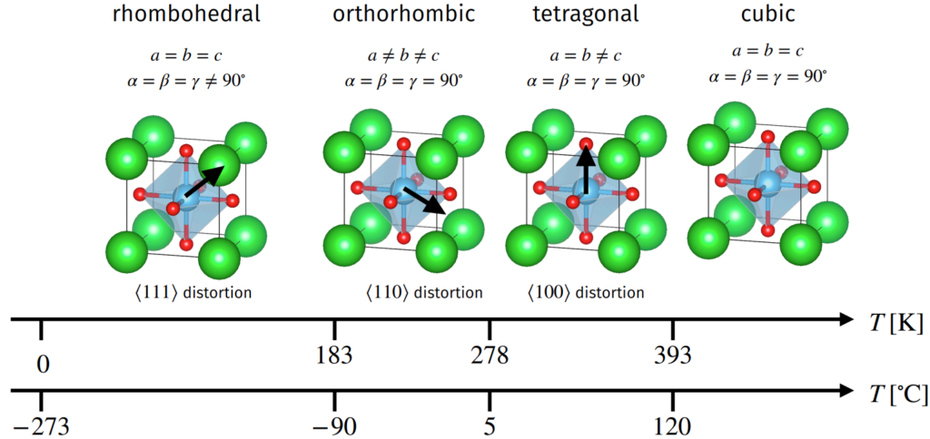
Perovskites are crystals with stoichiometry $\text{ABX}_3$ for $\text{A,B}$ metal cations and $\text X$ an anion. The Goldschmidt tolerance factor measures how distorted from a cubic crystal structure the perovskite is, $\Delta_{\text{cubic}}=\frac{R_A+R_X}{\sqrt{2}(R_B+R_X)}$.
Barium titanate $\text{BaTiO}_3$ is a ferroelectric perovskite with $\Delta_{\text{cubic}}\approx 1.07$ so $\text{Ba}^{2+}$ cations too large, lot of space for $\text{Ti}^{4+}$ cation to polarize in the octahedral interstice. As a result, at temperatures $T<T_C=120^{\circ}\text{C}$ such as room temperature $T=20^{\circ}\text C$ it exhibits ferroelectric hysteresis. Specifically, cooling from $T=T_C$, it undergoes a paraelectric-to-ferroelectric first-order phase transition in its 3D Bravais lattice $\Lambda_{\text{pc}}\mapsto\Lambda_{\text{bct}}$ (and goes into other ferroelectric phases at lower temperatures still).

Landau theory can be used to explain semi-quantitatively the phenomenology of phase transitions. The idea is to postulate an ansatz for the Helmholtz free energy $F:=U-TS$ and to then seek to minimize it (why not Gibbs free energy instead?) with respect to temperature $T$ and an order parameter $P$ (the induced polarization in this case).
Ferroelectrics are not necessarily monodomain (unless $|\textbf E^{\text{ext}}|$ is sufficiently strong), but more commonly have many polarization domains separated by polarization domain walls due to an energetic competition between $V_{\text{dipoles}}$ and $V_{\text{stray}}$ (and it is the pinning of polarization domain walls by defects that gives rise to the irreversibility of ferroelectric hysteresis in the first place).
Ferroelectrics are useful for $2$ main reasons: they have large polarizability $\varepsilon$ so are used as dielectrics in capacitors, and because of their ferroelectric hysteresis properties for ferroelectric RAM, etc.
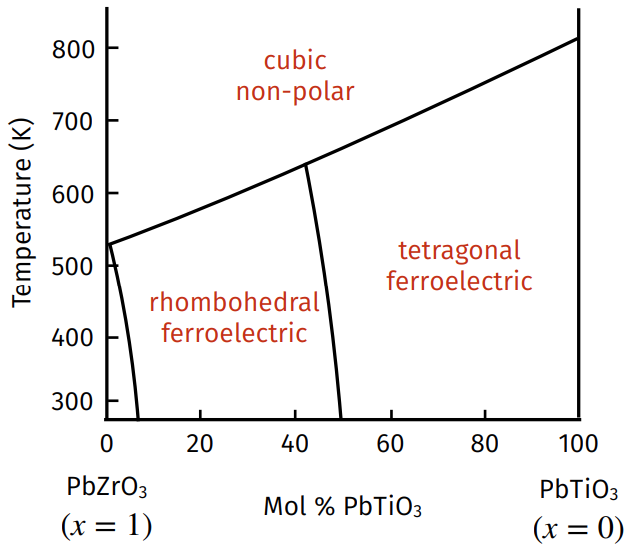
Another ferroelectric “perovskite” is lead zirconate titanate (PZT) $\text{PbZr}_x\text{Ti}_{1-x}\text O_3$ where $x\in[0,1]$, with the important composition being around $x\approx 0.5$ at room temperature due to the presence of a morphotropic phase boundary there (the central $\text{Ti}^{4+}$ cation can be polarized in a total of $|\{100\}|+|\{110\}|=6+8=14$ distinct directions).

The magnetization field $\textbf M:=n\boldsymbol{\mu}$ is the density of magnetic dipoles (analogous to the polarization density $\textbf P:=n\textbf p$ as the density of electric dipoles).
Magnetic susceptibility is defined by $\textbf M^{\text{ind}}=\chi_m\textbf H^{\text{ext}}$.
Using $\textbf M$, magnetic properties of materials can be classified into $5$ buckets: diamagnetic, paramagnetic, ferromagnetic, antiferromagnetic, and ferrimagnetic, where both ferromagnetic and ferrimagnetic materials have hysteresis loops:

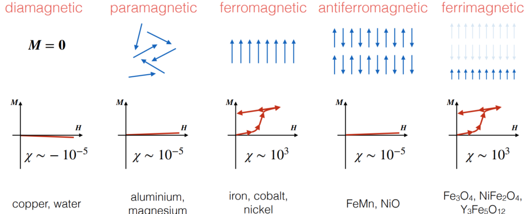
For example, magnetite (where magnetism was discovered) is a ferrimagnetic material adopting an inverse spinel crystal structure.
Fundamentally, the origin of magnetism in matter is due to the exchange interaction energy and the Pauli exclusion principle (so parallel spins are energetically favorable to minimize exchange interaction energy, but this is in competition with thermal energy/entropic considerations that wants to randomize magnetic moments) hence existence of a Curie temperature $T_C$ such that for $T>T_C$, magnetization vanishes via a ferromagnetic-to-paramagnetic phase transition.
Ferromagnets have easy and hard axes due to magnetocrystalline anisotropy, and these easy and hard axes also give rise to shape anisotropy (e.g. explains why bar magnets and not “fat magnets”).
Ferromagnets exhibit magnetostriction.
For analogous energy competition reasons as ferroelectrics, ferromagnets also have magnetization domains separated by domain walls, and the reason for irreversible ferromagnetic hysteresis (domain wall pinning) is identical.
Ferromagnets subdivide into soft and hard ferromagnets, soft ferromagnets are important for transformers (need to be able to easily switch magnetization back and forth) whereas hard ferromagnets have microstructure engineered to deliberately pin domain wall motion (e.g. neodymium magnets).
Ionic conductors are described in the steady state by the Fick-Ohm-Boltzmann equation (called Nernst-Einstein equation for some reason) $\frac{\sigma_{\infty}}{D_{\infty}}=\frac{nq^2}{kT}$.
Two important stochiometric defects are Schottky defects (simultaneous cation and anion vacancies) and Frenkel defects (an ion moves into an interstice, leaving behind a vacancy). The presence of such vacancies allows small ions to jump, mediating conduction. However, the jump is thermally activated (need enough thermal energy, described by Arrhenius equation $D=D_0e^{-\Delta E_a/RT}$, so ionic conduction works best when served hot!
Doping zirconia (zirconium dioxide) $\text{ZrO}_2$ with yttrium $\text Y^{3+}$ cations forces creation of $\text{O}^{2-}$ vacancies for charge neutrality. These vacancies mean that yttria-stabilized zirconia (YSZ) is an ionic conductor (called “stabilized” because the yttrium also stabilizes the otherwise unstable high-temperature cubic phase of zirconia).
Bismuth oxide $\text{Bi}_2\text O_3$ in its cubic ($\delta$) phase is also an ionic conductor.
Ionic conductors are useful electrolytes in oxygen concentration cells for $\lambda$-sensors as vehicle exhaust control systems, and hydrogen fuel cells for the hydrogen economy.
Expected end-to-end distance in an $N$-monomer polymer chain is $\sqrt{N}\ell_K$, where $\ell_K$ is the Kuhn length of the polymer chain.
Polymers have an inherent anisotropy to them, this leads to their birefringence $\Delta n:=n_{\text{slow}}-n_{\text{fast}}$ (and remember $n=\sqrt{\hat{\mu}\hat{\varepsilon}}$). Rotation angle of birefringence is $\Delta\theta=k\Delta_{\gamma}x=2\pi\Delta n\Delta x/\lambda$. Typically studied under crossed polarizers, for white light source, the color blocked is complementary of color observed (as given on a Michel-Levy chart). For crossed polarizers, irradiance of all wavelengths also varies as $\cos^2(\theta)$ (get extinction positions), enabling determination of fast and slow axes. To determine exactly which is which, use a compensator.
Polymers are examples of liquid crystals, formed at intermediate temperatures and classified by a unit director field $\textbf D$ (don’t confuse with electric displacement field) and order parameter $Q=\overline{P_2(\cos(\theta))}$ into nematic, smectic A/C, and chiral nematic (pitched/helical) liquid crystals. As with alignment of polarization domains in ferroelectrics or magnetization domains in ferromagnets, the same energy competition (alignment vs. thermal) drives the phase transitions (similarly get domain walls as seen in Schlieren textures, but these are now called disclinations where get Schlieren brushes). Unit director field $\textbf D$ also defines slow and fast axes for birefringence of liquid crystals.
A chiral nematic liquid crystal can be enforced using Dirichlet boundary conditions on the unit director field $\textbf D$, and an external $\textbf E^{\text{ext}}$-field can be applied to such a chiral nematic liquid crystal pixel to induce a Freedericksz ON/OFF phase transition, the key buzzword behind liquid crystal displays (LCDs).

Diffraction

X-rays are arguably the most important experimental tool in crystallography (and other fields of science such as chemistry and biology). The reason is that their wavelengths $\lambda\sim 1 A$ just happens to coincide with the typical length scale of most of these crystal structures and molecules, etc. that one is interested in understanding the structure of so that they will indeed be resolvable. Typical source of x-rays include $\text{Cu}$ $K_{\alpha}$ with $\bar{\lambda}\approx 1.542 A$.
For single crystals $\Gamma$, the rule is that the lattice plane $(hkl)$ will usually diffract x-rays incident on the plane (in accordance with the Bragg equation $\lambda=2d_{hkl}\sin(\theta_{hkl})$) unless the structure factor $\psi_{hkl}=0$ vanishes (in which case $(hkl)$ is said to be systematically absent, and different 3D Bravais lattices $\Lambda$ have different selection rules about which lattice planes should or shouldn’t be systematically absent).
For polycrystals, typically have a powder of the polycrystalline material, hence called x-ray powder diffraction. Due to randomness of grain orientations, get both front and back reflections via Debye-Scherrer cones and irradiance $I\propto |\{hkl\}||\psi_{hkl}|^2$ as in the Born rule. Can be imaged using a Debye-Scherrer camera on photographic film or using an electronic detector.
In general, any kind of photographic film or “sampling” of an interference pattern should be thought of as a slice through the reciprocal lattice $\Lambda^*$ of the original 3D Bravais lattice $\Lambda$. Bragg’s law has a nice interpretation in $\Lambda^*$ via the Ewald sphere construction.
Transmission electron microscopy and scanning electron microscopy take advantage of the even finer de Broglie wavelength of electrons to image at even higher resolutions.

Microstructure

To image the microstructure of a material, can use reflected light microscopy (need a chemical etchant like Nital first to etch different phases at different rates), or for greater resolution, use SEM or atomic force microscopy (AFM).
Gibbs free energy $G:=H-TS$ is minimized at constant $p$ and $T$. Thus, there is often an enthalpic ($H$) and entropic ($-TS$) competition that determines the equilibrium phases of a material at given conditions, with the general theme being that in the hot limit $T\to\infty$, entropic effects dominate whereas in the cold limit $T\to 0$ enthalpic effects dominate.
Since $dG=Vdp-SdT$, it follows that the slope $\left(\frac{\partial G}{\partial T}\right)_p=-S<0$ is always negative. For two phases, the temperature $T_{12}$ at which $G_1=G_2$ is the phase transition temperature between those phases (although this is for equilibrium only; phase diagrams only show equilibrium phases of globally minimum $G$, but metastable phases of locally minimum $G$ can persist if there is sufficient activation energy barrier).
For any solution of two atomic species $A,B$, the Gibbs free energy of mixing is $\Delta G_{\text{mix}}=\Delta H_{\text{mix}}-T\Delta S_{\text{mix}}$. Assuming only nearest-neighbor interactions matter, then $\Delta H_{\text{mix}}=H_{\text{sol}}-H_{\text{mech mix}}=\lambda_{AB}x_Ax_B$ where $x_A=n_A/n,x_B=n_B/n$ are mole fractions and $\lambda_{AB}\sim nC(2H_{AB}-H_{AA}-H_{BB})$ is the $AB$-interaction parameter and $C$ is a coordination number. Meanwhile, ignoring thermal contributions to entropy, $\Delta S_{\text{mix}}=S_{\text{sol}}-S_{\text{mech mix}}=-nR(x_A\ln(x_A)+x_B\ln(x_B))$ is just a linear combination. The solution is ideal iff $\Delta H_{\text{mix}}=\lambda_{AB}=0$ (meaning that $A$ and $B$ are probably quite similar) and regular otherwise. Thus, the regular solution model “Lagrangian” is: $$\Delta G_{\text{mix}}=\lambda_{AB}x_Ax_B+nRT(x_A\ln(x_A)+x_B\ln(x_B))$$
If $\lambda_{AB}\leq 0$, then $\Delta G_{\text{mix}}<0$ always, and
The more interesting case is $\lambda_{AB}>0$ since then at low $T$ the enthalpic term dominates and segregation of phases occurs whereas at high $T$ the entropic term dominates again and get a uniform solution once more.
Regular solution model is only an approximation, has many assumptions built into it.
In practice, determine compositions by using a phase diagram and proportions using tie lines and lever rule.
Eutectic phase transitions are of the form $L\to\alpha+\beta$, and generally have a lamellar microstructure/intergrowth due to cooperative diffusive growth. Are important in solder, where a low melting point is desirable (melting point of eutectic alloy of solder is lower than either of the pure metals).
Experimentally, phase diagrams can be mapped out by measuring cooling curves $T(t)$ for a given composition of two atomic species. Changes in the cooling rate $\dot T$ suggest phase transitions, and $\dot T=0$ is a hallmark of eutectic solidification $L\to\alpha+\beta$.
Rapid/non-equilibrium solidification leads to coring of the solid that is solidified. Such solids may also be dendritic in nature.
So far have just considered thermodynamics, need consider kinetics too. Homogeneous nucleation of a solid phase $\alpha$ in a liquid $L$ (both of the same composition), the driving force $\Delta G_V$ for a supercooling of $\Delta T<0$ is $\Delta G_V=\Delta T\Delta S_V$ (assuming the heat capacity $C_p$ is independent of $T$), and so spherical nucleation is governed by a “Lagrangian” $\Delta G(r)=\frac{4}{3}\pi r^3\Delta G_V+4\pi r^2\gamma$ with the work of nucleation being $\Delta G^*=16\pi\gamma^3/(3\Delta G_V^2)$ (note the essential proportionalities) and $r^*=-2\gamma/\Delta G_V$ (again, the proportionalities should make sense).
Nucleation rate (nucleations per unit volume per unit time) varies with temperature $T$ as: $\dot{N}(T)\propto N_Se^{-\Delta G^*(T)/RT}e^{-E_a/RT}$, where the notation $\Delta G^*(T)$ emphasizes that the driving force also depends on $T$ via the supercooling $\Delta T=T-T_m$.
Heterogeneous nucleation substantially smaller energetic barrier and therefore faster $\dot N$.
When a solid phase $\alpha$ nucleates inside another solid phase $\beta$ (not liquid), no longer a sphere (as it was for a liquid), instead need consider coherency of interfaces. Incoherent interfaces have high surface energy $V_{\gamma}\propto\gamma$, so tend to try and minimize incoherent surface area and therefore (counterintuitively) want to grow in the direction of incoherent interfaces.
$\Gamma_{\text{Widmanstatten}}$ is a crystal structure found in certain $\text{Fe}$-$\text{Ni}$ meteorites with sufficiently slow cooling rate $\dot T$, shows how $\Lambda_{bcc}$ and $\Lambda_{fcc}$ iron-rich phases can have coherent interface.
Isothermal Transformation (TTT) Diagrams are for a fixed composition.
Displacive phase transitions (e.g. austenitic fcc steel undergoing a martensitic bct phase transition) are in contrast to reconstructive phase transitions.
The standard phase diagram for the $\text{Fe}$-$\text{C}$ alloy system is actually only a quasi-equilibrium phase diagram. Cast irons have $2%<w_{\text{C}}<4\%$ whereas steels have $0.1%<w_{\text{C}}<1.5\%$ and the latter are dominated by a eutectoid phase transition to form pearlite = ferrite + cementite.
With steels however, there is a lot of metallurgical wisdom that has been gathered over the years on ways to manipulate the steel to get more properties out of it.
To harden a steel, the standard 3-step recipe is: anneal, quench, temper. First, anneal the steel up into the austenitic $\gamma$ phase and wait until it equilibrates. Then quench it rapidly in water. This prevents the interstitial carbon $\text C$ atoms from diffusing to form the lamellar eutectoid microstructure and instead results in them occupying octahedral interstices in a bct $\text{Fe}$ matrix. This $\Lambda_{\text{bct}}$ is thus considerably strained, impeding dislocation motion (so hard) but also brittle. To reduce brittleness while maintaining hardness, tempering is used (hold at some sub-eutectoid $T$) to introduce small cementite precipitates in ferrite matrix (very different from how it would look for eutectoid phase transition).

Al-Cu alloy system is important in aerospace engineering applications.
In general, strength $\sigma_y$ increases with smaller grains $d$ via the Hall-Petch equation $\sigma_y=\sigma_0+k/\sqrt{d}$ (grains impede dislocation glide), hence the fuss about finer microstructure.
Al-Cu alloys undergo the same 3-step processing to harden them: anneal, quench, temper. In this third tempering step, the incoherent tetragonal structure of the $\theta$ phase means that several intermediate metastable phases form first: GP zones, $\theta”$, $\theta’$ and finally $\theta$, becoming more and more incoherent.

Mechanical Behavior of Materials

For uniaxial loading along some lattice direction in a crystal, can experimentally measure a stress-strain curve or $\sigma^{\text{ext}}$-$\varepsilon^{\text{ind}}$ curve. In fact, in the elastic deformation regime defined by small external stress $\sigma^{\text{ext}}$, the strain increases linearly in accordance with Hooke’s law $\varepsilon^{\text{ind}}=\frac{\sigma^{\text{ext}}}{E}$ where $E$ is Young’s modulus. Atomic origin of this linearity can be attributed to quadratic nature of Lennard-Jones potential energy at the equilibrium distance $r_0$, and pursuing this line of reasoning fully, one even estimates $E\sim\frac{1}{r_0}\frac{d^2V}{dr^2}(r_0)$ so that sharper potential wells and closer-packed lattice planes mean stiffer materials.
Beyond the yield stress $\sigma^{\text{ext}}_y$, materials undergo irreversible plastic deformation (cf. so many of the other irreversible phenomena in this course notably ferroelectric and ferromagnetic hysteresis). Fundamental insight is that the origin of such plastic deformation turns out to be due to dislocation glide on close-packed lattice planes and in close-packed lattice directions in crystals, providing low-energy-cost way for whole a** lattice planes to effectively glide and thereby leading to plastic deformation.
Poisson’s ratio is roughly speaking $\nu:=-\frac{\varepsilon_{\rho}^{\text{ind}}}{\varepsilon_{z}^{\text{ext}}}$ in the limit of small external strains (really external stresses). Metals usually have $\nu\approx 0.3$, and $nu=0.5$ is the condition for incompressibility (e.g. rubbers).
Ductility is measured by the failure strain $\varepsilon_f$. Ductile materials have large $\varepsilon_f$ whereas brittle materials have low $\varepsilon_f$.
Analogous relation for shear stresses and their induced shear strains: $\gamma^{\text{ind}}=\frac{\tau^{\text{ext}}}{G}$ where $G$ is the shear modulus.
Note that $E=2G(1+\nu)$ so the $3$ are not independent of each other.
Total strain energy density is $u=\frac{1}{2}E\varepsilon^2+\frac{1}{2}G\gamma^2$.
In many materials, Young’s modulus $E$ (and I would imagine shear modulus $G$) is a tensor field due to anisotropy, for instance in fiber composites. Can use the Voigt or Reuss models to estimate the Young’s moduli parallel and perpendicular to the fibers based on volume fractions of fiber and matrix (although not super accurate).
Phenomenon of thermal expansion (and its linear nature over most temperature ranges) can be rationalized via the asymmetry of the LJ potential (think of as a ball rolling back and forth down the potential well). Leads to thermal stresses in bimetallic strips and any interface of two different metals joined together.
Euler-Bernoulli beam theory.
Important: Experimentally, plastically deformed materials appeared to have parallel stripes on their surfaces when loaded axially $\sigma^{\text{ext}}$.

Closer examination showed that each stripe was like a little stair on a staircase (will turn out to be of magnitude $|\textbf b|$); lattice planes of that specific orientation had seemed to glide ever so slightly, and this was what caused the plastic deformation. But if one naively adapts a block-slip model of calculating the critical shear stress $\tau^*$ needed to move a lattice plane over another lattice plane, one obtains values that far exceed experimental observations. Turns out there is a loophole, a way to make it seem as if an entire lattice plane had slid across another one, but requiring far less stress (Peierls-Nabarro stress $\sim Ge^{-2\pi w/|\textbf b|}$). Dislocations (ruck through carpet analogy)! Most materials contain dislocations (and indeed, very pure materials with no dislocations can approach the block-slip $\tau^*$).

Dislocations $:=$ 1D (line) defects (cf. vacancies as 0D defects, cracks as 2D defects?). Thus, dislocations are a subset of defects.
Edge dislocations have line vector $\boldsymbol{\ell}$ along the bottom of the extra half-plane of atoms, and Burgers vector $\textbf b\in\Lambda$ orthogonal to it (complete the Burgers circuit).
Also have screw dislocations where $\boldsymbol{\ell}$ is along the helical “screw axis” and Burgers vector $\textbf b$ now parallel to $\boldsymbol{\ell}$ by the magnitude of the dislocation.
Most dislocations have both edge character and screw character (cf. hybrid atomic orbitals having $s$ character and $p$ character). However all dislocations, regardless of their exact edge/screw character give the same net effect of making lattice planes glide (ruck in the carpet again!) and glide on the glide plane $\text{span}_{\textbf R}(\textbf b,\textbf{\ell})$ provided there is sufficient shear stress (much less than the block-slip model, but still non-zero as determined by projecting the external tensile stress $\sigma^{\text{ext}}$ onto the lattice plane to obtain a resolved shear stress $\tau^{\text{ind}}=\sigma^{\text{ext}}\cos(\phi)\cos(\lambda)$). Note that $\lambda$ and $\phi$ are not in general complementary angles, rather I believe $90^{\circ}\leq\lambda+\phi\leq 180^{\circ}$.
Dislocation loops can either be vacancy loops or interstitial loops.
A dislocation can be thought of as having a free body diagram consisting of a fictitious “glide force” (not fictitious in the sense of non-inertial but just actually fictitious because dislocations are not actual objects) and some resistive drag force. The glide force $\textbf f$ is a force per unit length (makes sense, dislocations are 1D defects) and is $\textbf f=\tau^{\text{ind}}\textbf b$.
Shear strain energy (per unit line vector length) stored in a screw dislocation is $V\approx \frac{1}{2}G|\textbf b|^2$. Edge dislocations have similar formula, and are more energetically costly than screw dislocations (per unit length).
For a given stress $\boldsymbol{\sigma}^{\text{ext}}$, the close-packed slip system to activate first will have the largest Schmid factor (i.e. closest to $\cos^(45^{\circ})=1/2$). For crystals $\Gamma$ admitting $\Lambda_{\text{bcc}}$ or $\Lambda_{\text{fcc}}$ 3D Bravais lattices, these are given conveniently by the OILS rule (why does it work?).
During loading, the slip direction rotates towards the tensile axis $\lambda\to 0$.
From the frame of the sample however, one can think of the tensile axis rotating towards the slip direction instead, and this is made explicit by adding multiples of the slip direction to the tensile axis until two of the indices of the rotated tensile axis have same components (at which point duplex slip is initiated on the two lattice planes with equal Schmid factor), and the tensile axis starts rotating toward the sum of their slip directions. Since number of lattice planes and interplanar spacing is assumed conserved during plastic deformation, it follows that one has the Heisenberg quantities $L\cos(\lambda)=\text{constant}$ and therefore by complementarity $L\sin(\phi)=\text{constant}$ (just think intuitively about these are referring to!).
Basically, to explain plastic deformation to a 5-year old, put your hands (lattice planes) together and show one “crawling” over the other (dislocation propagating like ruck in carpet).
For $\Gamma_{\text{hcp}}$, there may be geometric softening in the plastic deformation regime.
For $\Gamma_{\text{fcc}}$, there are $3$ stages of plastic deformation: constant $\sigma$ (easy glide), followed by work hardening, followed by cross slip (occurs earlier for higher stacking fault energies because partial dislocations are less separated and need to combine since they are not pure screw character). In polycrystals, the average Schmid factor is called the Taylor factor, and is $\overline{\cos(\phi)\cos(\lambda)}=\frac{1}{3}$ but this does not yield an accurate prediction of yield stress $\sigma_y$ due to grain boundary influence (Hall-Petch).
For $\Gamma_{\text{polycrystalline}}$, duplex slip (and thus work hardening) initiates at different stresses in different grains of the polycrystal, so get continuous work hardening.
In a nutshell, work hardening is associated with duplex slip and is when dislocations react to become sessile, impeding other dislocations and therefore strengthening the material.
Dislocations are like stress dipoles—>form dislocation arrays.
When dislocations meet, they either cut/intersect (i.e. make a jog of length $J_1=|\textbf b_2|$ which may or may not be glissile) or combine. Combination occurs iff Frank’s rule $\textbf b_1\cdot\textbf b_2<0$ is satisfied (i.e. energetically favorable, minimizes the total amount of “dislocation”). Intuitively, $\textbf b=\textbf b_1+\textbf b_2$ and $\boldsymbol{\ell}$ must lie on the intersection of the two slip planes (use Weiss zone law or just cross product). If the new $\text{span}_{\textbf R}(\textbf b,\boldsymbol{\ell})$ is not a close-packed lattice plane, then get a sessile/forest Lomer lock. This then impedes other dislocations on same plane—>work hardening.
Dislocations are generated by Frank-Read sources (Discord symbol).
Edge dislocations can bypass obstacles by dislocation climb (sinking and sourcing vacancies). (Perfect) screw dislocations can bypass obstacles by cross slip (because $\textbf b\times\boldsymbol{\ell}=\textbf 0$ for screw dislocations, can glide on any crystallographically equivalent lattice planes provided sufficient external stress).
Strengthen = increase $\sigma_y$ (super duper important for engineering b/c want stuff to operate in the linear elastic regime; in some sense, all this stuff about plastic deformation we’ve been learning is just a whole lot of shit that an engineer would want to avoid by keeping everything nice and simple and elastic).
Dislocation density $\rho$ is meters of dislocation line (again dislocations are 1D defects!) per meter cubed.
Grain boundaries obviously inhibit dislocation glide (get pile up). Smaller grains have shorter pile-up, so stronger (Hall-Petch).
Another way to strengthen a material is by alloying with solute/impurity atoms. This is solid solution strengthening. For substitutional solute atoms, their stress field symmetrically sucks in dislocations, but the strengthening is modest. For interstitial solute atoms, strain field can be asymmetric (e.g. $\text{C}$ solute atoms in octahedral interstices of $\alpha$-$\text{Fe}$ matrix of a low-carbon steel, asymmetry allows interaction with both edge and screw dislocations). Furthermore, interstitial diffusion much faster than substitutional diffusion. Thus, interstitial solid solution strengthening $\gg$ substitutional solid solution strengthening.
For low-carbon steels specifically, the rapid interstitial diffusion of $\text{C}$ atoms to dislocations forms Cottrell atmospheres. For low-carbon steels, also get a phenomenon of Luders bands which are boundaries separating yielded (near ends, where dislocations have escaped from Cottrell atmospheres) and unyielded (near middle, where they haven’t yet) regions which merge toward each other, requiring reduced yield stress.
At low $T$ (e.g. room temperature), the Cottrell atmosphere effect with Luders bands was described. At high $T$, carbons are so mobile they just move along with dislocations so no strengthening (get a vanilla stress-strain curve). At intermediate $T$, get Portevin-Le Chatelier effect (trap-escape cycle of dislocations from Cottrell atmospheres—>serrations in stress-strain curve).
Precipitate strengthening means using a whole other phase (not just solute atoms like C in steel, but a whole fricking other phase). For small precipitates, dislocations have to cut through them, increasing strengthening by $\Delta\sigma_y\propto\sqrt{r}$. For large precipitates, dislocations can get away by Orowan bowing around them $\Delta\sigma_y\propto \frac{1}{r}$, leaving two dislocation loops (thus increasing dislocation debris). For a dislocation of Burgers vector $\textbf b$ in a material of shear modulus $G$, $\tau_{\text{bow}}\propto\frac{G|\textbf b|}{L}$ so farther spaced precipitates require less stress to bow across.
When tempering martensite to nucleate $\text{Fe}_3\text C$ precipitates in $\alpha$, one has $\Delta\sigma_y(t_{\text{aging}})$, first solid solution strengthening, then coherency strains, then cutting, and finally bowing (at which point the material would be considered overaged).
Dissociation (opposite of combining!) of (perfect) dislocation into partial dislocations in $\Lambda_{\text{fcc}}$ is favorable due to Frank’s rule. They will normally have a repulsive interaction between each other, but also their separation is limited by the stacking fault energy of the stacking fault between them, so that higher stacking fault energy means earlier stage-III cross slip in their plastic deformation.
Order hardening is a functor from disordered solid solutions to ordered solid solutions below a certain temperature $T$, where the ordered, low-$T$ phase is much stronger (hence the name) due to formation of anti-phase boundaries and the associated energy cost of that.
So…I’ve been emphasizing how plastic deformation is mainly driven by dislocation glide…yes, that’s true, a more minor way it could happen is via deformation twinning (simultaneous shearing of successive lattice planes with mirror symmetry about twin boundaries). For example, for $\Lambda_{\text{fcc}}$, deformation twinning happens along $\{111\}$ close-packed lattice planes by a downward amount $\frac{a}{6}\langle 11\bar{2}\rangle$ from a B position to a C position sort of thing (identical as in dissociation into partial dislocations).
There are also annealing twins.
Toughness = Ductility (opposite of brittle)
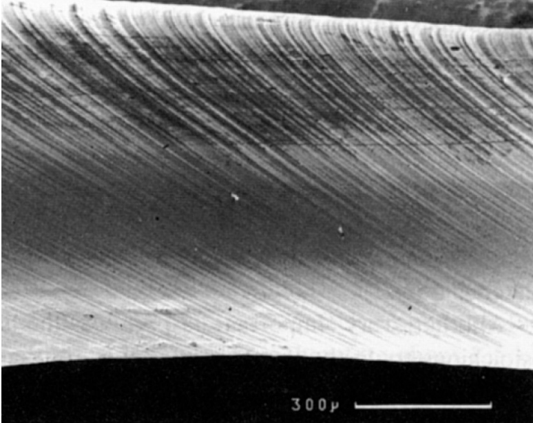
Just as block slip model overestimates stress needed to plastically deform, so naive breaking-plane-of-bonds model overestimates stress needed to fracture. For former, the loophole was dislocations (1D defects). For the latter, it is cracks (2D defects).
Griffith criterion for energy balance, propagation of crack favorable. Griffith criterion is easiest to apply for brittle materials, where $G\geq G_C= 2\gamma$. For ductile materials, there is a zone plasticity ahead of crack tip, blunting it, but therefore requiring extra work to be done (larger strain energy release rate $G$ needed).
Plotting impact energy (a proxy for toughness) $E_{\text{impact}}(T)$ as a function of temperature $T$, see that for metals with $\Lambda_{\text{bcc}}$, get a ductile-to-brittle transition temperature $T_{d\to b}$ (think steels and the Titanic in those cold arctic waters where the steel was brittle).
Fiber-matrix composites may paradoxically have both the fibers and matrix individually being brittle yet the composite being tough (sum of parts is not whole!). This is due to strengthening effect from the fiber pull-out mechanism.
In a pressurized pipe, the hoop stress is twice the axial stress, so pipes burst longitudinally.

Leave a Reply Cancel reply

Archives

Meta