The purpose of this post is to explain the \(2\) key models of classical optics, namely geometrical optics (also known as ray optics) and physical optics (also known as wave optics). Although historically geometrical optics came before physical optics, and indeed this is also usually the order in which they are conventionally taught, this post will take the more unconventional approach of presenting physical optics first, and then showing how it reduces to geometrical optics in the \(\lambda\to 0\) limit.
Physical Optics
Maxwell’s equations assert that the electric and magnetic field \(\textbf E,\textbf B\) satisfy vector wave equations in vacuum:
\[\biggr|\frac{\partial}{\partial\textbf x}\biggr|^2\textbf E-\frac{1}{c^2}\ddot{\textbf E}=\textbf 0\]
\[\biggr|\frac{\partial}{\partial\textbf x}\biggr|^2\textbf B-\frac{1}{c^2}\ddot{\textbf B}=\textbf 0\]
Any of their \(6\) components (denoted \(\psi\)) thus satisfy the scalar wave equation \(|\frac{\partial}{\partial\textbf x}|^2\psi+\frac{1}{c^2}\ddot{\psi}=0\). The spacetime Fourier transform yields the trivial dispersion relation \(\omega=ck\) from which it is evident that performing just a temporal Fourier transform (to avoid the minutiae of \(t\)-dependence) leads to the scalar Helmholtz equation for \(\psi(\textbf x)\):
\[\left(\biggr|\frac{\partial}{\partial\textbf x}\biggr|^2+k^2\right)\psi=\textbf 0\]
In other words, one is looking for eigenfunctions of the Laplacian \(\biggr|\frac{\partial}{\partial\textbf x}\biggr|^2\) with eigenvalue \(-k^2\). To begin, consider one of Green’s identities, valid for arbitrary scalar fields \(\psi(\textbf x’),\tilde{\psi}(\textbf x’)\) which are \(C^2\) everywhere in the volume \(V\):
\[\iint_{\textbf x’\in\partial V}\left(\psi\frac{\partial\tilde{\psi}}{\partial\textbf x’}-\tilde{\psi}\frac{\partial\psi}{\partial\textbf x’}\right)\cdot d^2\textbf x’=\iiint_{\textbf x’\in V}\left(\psi\biggr|\frac{\partial}{\partial\textbf x’}\biggr|^2\tilde{\psi}-\tilde{\psi}\biggr|\frac{\partial}{\partial\textbf x’}\biggr|^2\psi\right)d^3\textbf x’\]
(it’s just the divergence theorem applied to the vector field \(\psi\frac{\partial\tilde{\psi}}{\partial\textbf x’}-\tilde{\psi}\frac{\partial\psi}{\partial\textbf x’}\)). It is now obvious that the volume integral will vanish if one then imposes that both \(\psi(\textbf x’)\) and \(\tilde{\psi}(\textbf x’)\) also satisfy the scalar Helmholtz equation. Given any point \(\textbf x\in\textbf R^3\), it is physically clear that the spherical wave Green’s function \(\tilde{\psi}(\textbf x’|\textbf x)=e^{ik|\textbf x-\textbf x’|}/|\textbf x-\textbf x’|\) is one possible (though certainly not a unique) solution to the scalar Helmholtz equation, provided one stays away from the singularity at \(\textbf x’=\textbf x\). This motivates the choice of volume \(V\) to be some arbitrary region but with an \(\varepsilon\)-ball cut around \(\textbf x\), in which case the volume integral can legitimately be taken to vanish over this choice of \(V\). In that case, the surface \(\partial V=S^2_{\varepsilon}\cup S\) can be partitioned into an inner surface \(S^2_{\varepsilon}\) and an outer surface \(S\):
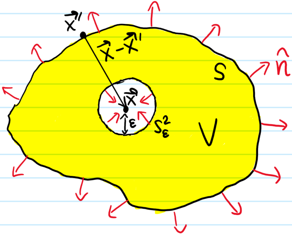
The flux through these two surfaces \(S^2_{\varepsilon},S\) must thus be equal:
\[\iint_{\textbf x’\in S^2_{\varepsilon}}\left(\psi\frac{\partial\tilde{\psi}}{\partial\textbf x’}-\tilde{\psi}\frac{\partial\psi}{\partial\textbf x’}\right)\cdot d^2\textbf x’=\iint_{\textbf x’\in S}\left(\tilde{\psi}\frac{\partial\psi}{\partial\textbf x’}-\psi\frac{\partial\tilde{\psi}}{\partial\textbf x’}\right)\cdot d^2\textbf x’\]
The integral over \(S^2_{\varepsilon}=\{\textbf x’\in\textbf R^3:|\textbf x’-\textbf x|=\varepsilon\}\) is straightforward in the limit \(\varepsilon\to 0\):
\[\iint_{\textbf x’\in S^2_{\varepsilon}}\left(\psi\frac{\partial\tilde{\psi}}{\partial\textbf x’}-\tilde{\psi}\frac{\partial\psi}{\partial\textbf x’}\right)\cdot d^2\textbf x’=\psi(\textbf x)\lim_{\varepsilon\to 0}4\pi\varepsilon^2\frac{1-ik\varepsilon}{\varepsilon^2}e^{ik\varepsilon}+\hat{\textbf n}\cdot\frac{\partial\psi}{\partial\textbf x’}(\textbf x)\lim_{\varepsilon\to 0}4\pi\varepsilon^2\frac{e^{ik\varepsilon}}{\varepsilon}=4\pi\psi(\textbf x)\]
One thus obtains Kirchoff’s integral formula for the scalar Helmholtz equation:
\[\psi(\textbf x)=\frac{1}{4\pi}\iint_{\textbf x’\in S:\textbf x\in V}\left(\frac{e^{ik|\textbf x-\textbf x’|}}{|\textbf x-\textbf x’|}\frac{\partial\psi}{\partial\textbf x’}-\psi(\textbf x’)\frac{\partial}{\partial\textbf x’}\frac{e^{ik|\textbf x-\textbf x’|}}{|\textbf x-\textbf x’|}\right)\cdot d^2\textbf x’\]
where as above:
\[\frac{\partial}{\partial\textbf x’}\frac{e^{ik|\textbf x-\textbf x’|}}{|\textbf x-\textbf x’|}=\frac{ik|\textbf x-\textbf x’|-1}{|\textbf x-\textbf x’|^3}e^{ik|\textbf x-\textbf x’|}(\textbf x’-\textbf x)\]
As an aside, Kirchoff’s integral formula is very similar in spirit to another more well-known integral formula, namely the Cauchy integral formula \(f(z_0)=\frac{1}{2\pi i}\oint_{z\in\gamma:z_0\in\text{int}(\gamma)}\frac{f(z)}{z-z_0}dz\) from complex analysis; the constraint of complex analyticity is analogous to constraining \(\psi\) to obey the Helmholtz equation; if one specifies both Dirichlet and Neumann boundary conditions for \(\psi(\textbf x’)\) everywhere on \(\textbf x’\in S\), then in principle this is enough to uniquely determine \(\psi(\textbf x)\) everywhere in the interior \(V\) of the enclosing surface \(S\).
Now consider the following standard diffraction setup:
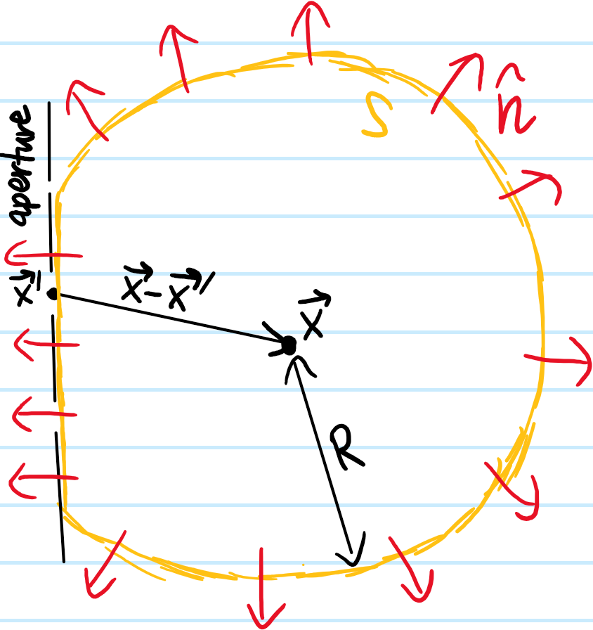
Here the surface \(S\) is chosen to be a sphere of radius \(R\) centered at \(\textbf x\), except where it flattens along the aperture with some distribution of slits. As one takes \(R\to\infty\), then in analogy to Jordan’s lemma from complex analysis, one can argue that the flux through this spherical cap portion of \(S\) in Kirchoff’s integral formula vanishes like \(\sim 1/R\to 0\) (this is admittedly still a bit handwavy, for a rigorous argument see the Sommerfeld radiation condition). Thus, the behavior of \(\psi\) on the aperture alone is sufficient to determine its value \(\psi(\textbf x)\) at an arbitrary “screen location” \(\textbf x\) beyond the aperture. Supposing a monochromatic plane wave \(\psi(\textbf x’)=\psi(x’,y’,0)e^{ikz’}\) of momentum \(k\) (hence solving the scalar Helmholtz equation) is normally incident on the aperture \(z’=0\) and that \(k|\textbf x-\textbf x’|\gg 1\) (easily true in most cases), this imposes the boundary condition \(-\frac{\partial\psi}{\partial z’}(x’,y’,0)=-ik\psi(x’,y’,0)\) so one can check that Kirchoff’s integral formula simplifies to:
\[\psi(\textbf x)\approx -\frac{ik}{4\pi}\iint_{\textbf x’\in\text{aperture}}\psi(\textbf x’)\frac{e^{ik|\textbf x-\textbf x’|}}{|\textbf x-\textbf x’|}(1+\cos\angle(\textbf x-\textbf x’,\hat{\textbf k}))d^2\textbf x’\]
Or equivalently:
\[\psi(\textbf x)=\frac{1}{i\lambda}\iint_{\textbf x’\in\text{aperture}}\psi(\textbf x’)\frac{e^{ik|\textbf x-\textbf x’|}}{|\textbf x-\textbf x’|}K(\textbf x-\textbf x’)d^2\textbf x’\]
where the obliquity kernel is \(K(\textbf x-\textbf x’):=\frac{1+\cos\angle(\textbf x-\textbf x’,\hat{\textbf k})}{2}=\cos^2\frac{\angle(\textbf x-\textbf x’,\hat{\textbf k})}{2}\). This is nothing more than a mathematical expression of the Huygens-Fresnel principle.
Fresnel vs. Fraunhofer Diffraction
In general the Huygens-Fresnel integral is difficult to evaluate analytically for an arbitrary point \(\textbf x\) on a screen. Thus, one often begins by making the paraxial approximation \(K(\textbf x-\textbf x’)\approx 1\iff |\textbf x-\textbf x’|\approx z\), except in the complex exponential (otherwise all Huygens wavelets would interfere constructively which is silly). Here instead, one implements a less strict version of the paraxial approximation in the form of a \(z^2\gg |\textbf x-\textbf x’|^2-z^2\) binomial expansion:
\[|\textbf x-\textbf x’|=\sqrt{z^2+|\textbf x-\textbf x’|^2-z^2}=z+\frac{|\textbf x-\textbf x’|^2-z^2}{2z}-\frac{(|\textbf x-\textbf x’|^2-z^2)^2}{8z^3}+…\]
In practice the quadratic term is negligible in the paraxial limit, so neglecting it and all higher-order terms yields the Fresnel diffraction integral:
\[\psi(\textbf x)=\frac{e^{ikz}}{i\lambda z}\iint_{\textbf x’\in\text{aperture}}\psi(\textbf x’)e^{ik(|\textbf x-\textbf x’|^2-z^2)/2z}d^2\textbf x’\]
Or equivalently, expanding \(|\textbf x-\textbf x’|^2=|\textbf x|^2+|\textbf x’|^2-2\textbf x\cdot\textbf x’\):
\[\psi(\textbf x)=\frac{e^{ikz}e^{ik(|\textbf x|^2-z^2)/2z}}{i\lambda z}\iint_{\textbf x’\in\text{aperture}}\psi(\textbf x’)e^{ik|\textbf x’|^2/2z}e^{-i\textbf k\cdot\textbf x’}d^2\textbf x’\]
where \(\textbf k=k\textbf x/z\). If in addition one also assumes that \(k|\textbf x’|^2/2z\ll 1\), then one obtains the Fourier optics case of far-field/Fraunhofer diffraction:
\[\psi(\textbf x)=\frac{e^{ikz}e^{ik(|\textbf x|^2-z^2)/2z}}{i\lambda z}\iint_{\textbf x’\in\text{aperture}}\psi(\textbf x’)e^{-i\textbf k\cdot\textbf x’}d^2\textbf x’\]
The reason that Fraunhofer diffraction is only considered to apply in the far-field is that the above condition for its validity can be rewritten as \(z\gg z_R\) where \(z_R:=\rho’^2/\lambda\) is the Rayleigh distance of an aperture of typical length scale \(\rho’\sim\sqrt{x’^2+y’^2}\) when illuminated by monochromatic light of wavelength \(\lambda\). In other words, the precise meaning of “far-field” is “farther than the Rayleigh distance \(z_R\)”. Otherwise, when \(z≲z_R\) then such a term cannot be neglected and one simply refers to it as Fresnel diffraction. Notice that \(z≲z_R\) is not saying the same thing as \(z\ll z_R\); it is often said that Fresnel diffraction is the regime of near-field diffraction but that phrase can be misleading because it suggests that \(z\) can be arbitrarily small, yet clearly at some point if one kept decreasing \(z\) then eventually the higher-order terms in the binomial expansion would also start to matter (moreover, the paraxial approximation would also start to break down). Instead of calling it “near-field diffraction”, a more accurate name for Fresnel diffraction would be “not-far-enough diffraction” \(z≲z_R\). By contrast, Fraunhofer diffraction truly is arbitrarily far-field \(z\gg z_R\). Of course nothing stops one from also considering the case \(z\ll z_R\), there just doesn’t seem to be any special name given to this regime and in practice it’s not as relevant. Finally, sometimes one also encounters the terminology of the Fresnel number \(F(z):=z_R/z\); in this jargon, Fraunhofer diffraction occurs when \(F(z)\ll 1\) whereas Fresnel diffraction occurs when \(F(z)≳1\).
In practice, one typically ignores the pre-factor in front of the aperture integrals since it is the general profile of the irradiance \(|\psi(\textbf x)|^2\) that is mainly of interest. In this case, particular for Fraunhofer diffraction, one can write \(\hat{\psi}(\textbf k)\equiv\psi(\textbf x)\) as just the \(2\)D spatial Fourier transform of the aperture.
Diffraction Through a Single Slit
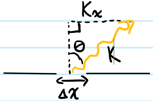
Consider a single \(y\)-invariant slit of width \(\Delta x\) centered at \(x’=0\). Then the Fraunhofer interference pattern has the form:
\[\hat{\psi}(k_x)\sim\int_{-\Delta x/2}^{\Delta x/2}e^{-ik_x x}dx=\frac{1}{ik_x}2i\sin\frac{k_x\Delta x}{2}\sim\Delta x\text{sinc}\frac{k_x\Delta x}{2}\]
where \(k_x=k\sin\theta\):
By contrast, the Fresnel interference pattern is given by:
\[\psi(x)\sim\int_{-\Delta x/2}^{\Delta x/2}e^{ik(x’-x)^2/2z}dx’\]
Although in general such an integral needs to be evaluated numerically, there is a simple geometric way to gain some intuition for how \(\psi(x)\in\textbf C\) behaves at fixed \(z≲z_R\sim\Delta x^2/\lambda\) via the Cornu spiral (also called the Euler spiral in contexts outside of physical optics). The idea is to shift the \(x\)-dependence from the integrand into the limits via the substitution \(\pi t’^2/2:=k(x-x’)^2/2z\iff t’=\sqrt{\frac{2}{\lambda z}}(x-x’)\). Then, ignoring chain rule factors, one has:
\[\psi(x)\sim\int_{t’_1(x)}^{t’_2(x)}e^{i\pi t’^2/2}dt’\]
where the limits are \(t’_1(x)=\sqrt{\frac{2}{\lambda z}}(x+\Delta x/2)\) and \(t’_2(x)=\sqrt{\frac{2}{\lambda z}}(x-\Delta x/2)\). Written in terms of the normalized Fresnel integral \(\text{Fr}(t):=\int_0^{t}e^{i\pi t’^2/2}dt’\):
\[\psi(x)\sim\text{Fr}(t’_2(x))-\text{Fr}(t’_1(x))\]
The object \(\text{Fr}(t)\) is a trajectory in \(\textbf C\) which is the aforementioned Cornu spiral:
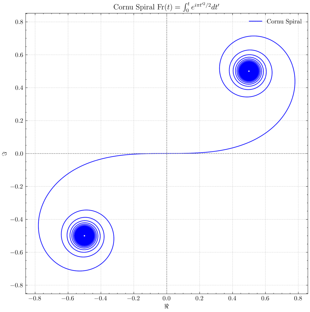
where one can check the limits \(\lim_{t\to\pm\infty}\text{Fr}(t)=\pm(1+i)/2\). Noting that \(\dot{\text{Fr}}(t)=e^{i\pi t^2/2}\), it follows that the speed \(|\dot{\text{Fr}}(t)|=1\) is uniform and thus the distance/arc length traversed in time \(\Delta t\) is always just \(\Delta t\). Moreover, the curvature \(\kappa(t)=\Im(\dot{\text{Fr}}^{\dagger}\ddot{\text{Fr}})/|\dot{\text{Fr}}|^3=\pi t\) increases linearly in the arc length \(t\) (essentially what defines a spiral!). The point is that the irradiance \(|\psi(x)|^2\sim|\text{Fr}(t’_2(x))-\text{Fr}(t’_1(x))|^2\) is now visually just the length (squared) of a vector between the points \(\text{Fr}(t’_1(x))\) and \(\text{Fr}(t’_2(x))\) on the Cornu spiral. The idea is to first trek a distance \(\frac{t’_1(x)+t’_2(x)}{2}=\sqrt{\frac{2}{\lambda z}}x\) from the origin to some central \(x\)-dependent point on the spiral, and then extend around it by the \(x\)-independent amount \(t’_1-t’_2=\sqrt{\frac{2}{\lambda z}}\Delta x\sim\sqrt{F(z)}\) to get a corresponding line segment whose length will be \(|\psi(x)|\).
Diffraction Through a Circular Aperture
Given a circular aperture of radius \(R\), its \(2\)D isotropic nature means that the Fraunhofer interference pattern is just proportional to the Hankel transform of the aperture:
\[\hat{\psi}(k_{\rho})\sim\int_{0}^R\rho’J_0(k_{\rho}\rho’)d\rho’\sim\frac{J_1(k_{\rho}R)}{k_{\rho}}\]
with \(k_{\rho}=k\sin\theta\). This is sometimes called a sombrero or \(\text{jinc}\) function, being the polar analog of the \(\text{sinc}\) function. It has its first zero at \(k_{\rho}R\approx 3.8317\) which defines the boundary of the Airy disk (cf. \(\text{sinc}(k_x\Delta x/2)\) having its first zero at \(k_x\Delta x/2=\pi\approx 3.1415\)). This is often expressed paraxially via the angular radius of the Airy disk \(\theta_{\text{Airy}}\approx 1.22\frac{\lambda}{D}\) with \(D=2R\) the diameter of the aperture (cf. \(\theta_{\text{central max}}\approx\frac{\lambda}{\Delta x}\) for the single slit).
For the same circular aperture setup, one can also ask what happens in the Fresnel regime \(z≲z_R\). In general, the integral is complicated:
\[\psi(\rho,z)\sim\int_0^R e^{ik\rho’^2/2z}\rho’ J_0(k_{\rho}\rho)d\rho’\]
But if one restricts attention to the symmetric case of being on-axis \(\rho=k_{\rho}=0\), then:
\[\psi(0,z)\sim e^{ikR^2/2z}-1\Rightarrow|\psi(0,z)|^2\sim\sin^2\frac{kR^2}{4z}\]
This is essentially the topologist’s favorite pathological sine function, but of course it was already mentioned that this solution is only reliable when the argument \(kR^2/4z\sim F(z)≳1\). For this specific on-axis case, it turns out one can significantly relax the paraxial assumption, namely, although one still assumes the obliquity kernel \(K(\textbf x-\textbf x’)\approx 1\), otherwise one acknowledges that \(r^2=\rho’^2+z^2\):
\[\psi(0,z)\sim\int_{z}^{\sqrt{R^2+z^2}}e^{ikr}dr\Rightarrow |\psi(0,z)|^2\sim\sin^2\frac{k(\sqrt{R^2+z^2}-z)}{2}\]
where if one were to binomial expand \(\sqrt{R^2+z^2}\approx z+R^2/2z\) one would just recover the Fresnel solution. If one fixes a given on-axis observation distance \(z\) and instead views \(|\psi(0,z)|^2\) as a function of the aperture radius \(R\) (and not \(z\)), then clearly it alternates between bright maxima and dark minima at aperture radii \(R\equiv\rho’_n\) given by:
\[\frac{k(\sqrt{{\rho’_n}^2+z^2}-z)}{2}=\frac{n\pi}{2}\iff \rho’_n=\sqrt{n\lambda z+\left(\frac{n\lambda}{2}\right)^2}\approx\sqrt{n\lambda z}\]
Thus, in general for a fixed aperture radius \(R\), there will be \(\sim F(z)\) concentric annuli of the form \(\rho’\in[\rho’_{n-1},\rho’_n]\) that can be made to partition the aperture disk; the annulus \([\rho’_{n-1},\rho’_n]\) is called the \(n\)-th Fresnel half-period zone. Note that the area of each Fresnel half-period zone is a constant \(\pi\lambda z\) in the Fresnel regime thus providing equal but alternating contributions to \(\psi(0,z)\) that lead to the observed oscillatory behavior in \(|\psi(0,z)|^2\). The existence of this Fresnel half-period zone structure motivates the construction of Fresnel zone plates which are vaguely like polar analogs of diffraction gratings, except rather than being regularly spaced, they block alternate Fresnel half-period zones with some opaque material to reinforce constructive interference for a given \(z\) and \(\lambda\) (thus, in order to design such a zone plate, one has to already have in mind a \(z\) and a \(\lambda\) ahead of time in order to compute the radii \(\rho’_n\approx\sqrt{n\lambda z}\) to be etched out). If a given \((z,\lambda)\) zone plate has already been constructed, but one then proceeds to move \(z\mapsto z/m\) for some \(m\in\textbf Z^+\), then in each of the Fresnel half-period zones associated to \(z\), there would now be \(m\) Fresnel half-period zones associated to \(z/m\), and so each transparent region of the \((z,\lambda)\) zone plate would allow through \(m\) of the \(z/m\) Fresnel half-period zones. Thus, if \(m\in 2\textbf Z^+-1\) is odd, then one would still expect a net constructive interference on-axis at \(z/m\), whereas if \(m\in 2\textbf Z^+\) then destructive interference of pairs of adjacent Fresnel half-period zones wins out (this parity argument is easy to remember because if \(m=1\) then nothing happens and the whole point of constructing the zone plate was to amplify the constructive interference at \(z\)). Finally, it is sometimes said that a given \((z,\lambda)\) Fresnel zone plate acts like a lens of focal length \(z\); however, due to the dependence on \(\lambda\), such a lens suffers from chromatic aberration.
Now consider the complimentary problem of calculating \(\tilde{\psi}(0,z)\) for a circular obstruction of radius \(R\), rather than a circular aperture of radius \(R\) carved into an infinitely-extending obstruction. Clearly, the two are related by subtracting the solution \(\psi(0,z)\) of the circular aperture of radius \(R\) from the free, unobstructed plane wave \(e^{ikz}\); this obvious corollary of the linearity of the scalar Helmholtz equation is an instance of Babinet’s principle. This leads to the counterintuitive prediction of Poisson’s spot (also called Arago’s spot):
\[\tilde{\psi}(0,z)=e^{ikz}-\psi(0,z)\sim e^{ik\sqrt{R^2+z^2}}\Rightarrow |\psi(0,z)|^2\sim 1\]
where, taking into account the obliquity kernel \(K(\textbf x-\textbf x’)\), this holds as long as one doesn’t wander too close to the aperture. Note from the earlier case of the circular aperture that there was the complementary (and equally counterintuitive) prediction that one could get a dark on-axis spot at certain \(z\) (i.e. those for which the aperture \(R=\rho’_{2m}\) partitions into an even number \(2m\) of Fresnel half-period zones as evident from the formula \(|\psi(0,z)|^2\sim\sin^2k(\sqrt{R^2+z^2}-z)/2\)).
Talk about how, by working with a scalar \(\psi\), have basically neglected polarization which only comes about from the vectorial nature of the electromagnetic field; forms basis of so-called scalar wave theory or scalar diffraction theory. Connect all this to the Lippman-Schwinger equation in quantum mechanical scattering theory (specifically, this is basically the first-order Born approximation solution to LS equation).
Fraunhofer is taxicab, treats wavefronts as planar, Fresnel is \(\ell^2\), actually considers their curvature. Actually, anywhere that Fraunhofer works, Fresnel also works.
Geometrical Optics
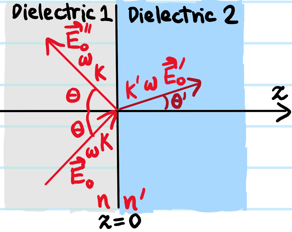
Consider a spherical glass of index \(n’\) and radius \(R>0\) placed in a background of index \(n\), and a paraxial light ray incident at angle \(\theta\) and distance \(\rho\) (where both \(\theta\) and \(\rho\) are measured with respect to some suitable choice of principal \(z\)-axis):
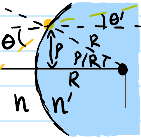
The incident angle of the yellow ray is \(\theta+\rho/R\) while its refracted angle is \(\theta’+\rho/R\) so Snell’s law asserts (paraxially) that:
\[n’\left(\theta’+\frac{\rho}{R}\right)=n\left(\theta+\frac{\rho}{R}\right)\]
This directly yields the paraxial ray transfer matrix for this spherical glass:
\[\begin{pmatrix}\rho’\\\theta’\end{pmatrix}=\begin{pmatrix}1&0\\ (n-n’)/n’R&n/n’\end{pmatrix}\begin{pmatrix}\rho\\\theta\end{pmatrix}\]
There is no need to memorize such a matrix; instead, because it is \(2\times 2\), it can always be quickly rederived by finding two linearly independent vectors on which the action of such a matrix is physically obvious. The natural choice are its eigenvectors, which correspond physically to the following two “eigenrays”:
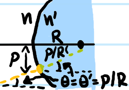
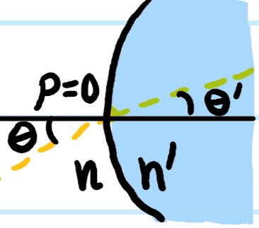
In the limit \(R\to\infty\) of a flat interface (e.g. in a plano-convex lens), the paraxial ray transfer matrix reduces to the diagonal matrix \(\begin{pmatrix}1&0\\ 0&n/n’\end{pmatrix}\).
Welding two such spherical glasses (of the same index \(n’\) and radii \(R>0,R'<0\) in the usual Cartesian sign convention) together back-to-back and assuming the usual thin-lens approximation (otherwise one would also need to include a propagation ray transfer matrix \(\begin{pmatrix}1&\Delta z\\ 0&1\end{pmatrix}\) if the thickness \(\Delta z>0\) were non-negligible), one obtains the paraxial ray transfer matrix of a thin convex lens (indeed any thin lens):
\[\begin{pmatrix}1&0\\ (n’-n)/nR’&n’/n\end{pmatrix}\begin{pmatrix}1&0\\ (n-n’)/n’R&n/n’\end{pmatrix}=\begin{pmatrix}1&0\\-P&1\end{pmatrix}\]
where \(P:=1/f\) is the optical power of the thin convex lens and the focal length \(f>0\) is given by the lensmaker’s equation:
\[\frac{1}{f}=\frac{n’-n}{n}\left(\frac{1}{R}-\frac{1}{R’}\right)\]
As a check of this formula’s self-consistency, consider the special case of a thin plano-convex lens (where the convex side has radius \(R>0\)). According to the lensmaker’s equation, this should have focal length \(1/f=(n’-n)/nR\). On the other hand, if one were to flip this plano-convex lens around (and call the radius of the convex side \(R'<0\)), then the lensmaker’s formula says it should now have focal length \(1/f’=-(n’-n)/nR’\). But, since both plano-convex lenses are thin, if one simply puts them next to each other then one would reform the thin convex lens as before, with effective focal length:
\[\frac{1}{f_{\text{eff}}}=\frac{n’-n}{n}\left(\frac{1}{R}-\frac{1}{R’}\right)=\frac{1}{f}+\frac{1}{f’}\]
In other words, the optical powers are additive \(P_{\text{eff}}=P+P’\). Note that this holds for any \(2\) thin lenses placed next to each other to form an “effective lens”, not just for the example of \(2\) plano-convex lenses given above. More generally, because the group of shears on \(\textbf R^2\) along a given direction is isomorphic to the additive abelian group \(\textbf R\), it holds for any \(N\in\textbf Z^+\) thin lenses arranged in an arbitrary order:
\[\begin{pmatrix}1&0\\-P_N&1\end{pmatrix}…\begin{pmatrix}1&0\\-P_2&1\end{pmatrix}\begin{pmatrix}1&0\\-P_1&1\end{pmatrix}=\begin{pmatrix}1&0\\-(P_1+P_2+…+P_N)&1\end{pmatrix}\]
It’s worth quickly clarifying why these are even thin lenses in the first place and why the claimed \(f\) really is a suitable notion of focal length. One can proceed axiomatically, demanding that a thin lens be any optical element which:
- Focuses all incident light rays parallel to the principal \(z\)-axis to a focal point \(f\) (i.e. \((\rho,0)\mapsto(\rho,-\rho/f)\)).
- Doesn’t affect any light rays that pass through the principal \(z\)-axis (i.e. \((0,\theta)\mapsto(0,\theta)\)).
These are two linearly independent vectors (though only the latter is an eigenvector, as shear transformations are famous for being non-diagonalizable), so these \(2\) axioms are sufficient to fix the form \(\begin{pmatrix}1&0\\-1/f&1\end{pmatrix}\) of the paraxial ray transfer matrix of a thin lens.
Often, one would like to use thin lenses to image various objects. Consider an arbitrary point in space sitting a distance \(\rho\) above the the principal \(z\)-axis and a distance \(z>0\) away from a thin lens. If a light ray is emitted from this point at some angle \(\theta\), and this light ray refracts through the thin lens (of focal length \(f\)), and ends up at some point \(\rho’,z’\) after the lens during its trajectory, then one has:
\[\begin{pmatrix}\rho’\\\theta’\end{pmatrix}=\begin{pmatrix}1&z’\\0&1\end{pmatrix}\begin{pmatrix}1&0\\-1/f&1\end{pmatrix}\begin{pmatrix}1&z\\0&1\end{pmatrix}\begin{pmatrix}\rho\\\theta\end{pmatrix}\]
where the composition of those \(3\) matrices evaluates to \(\begin{pmatrix}1-z’/f&z+z’-zz’/f\\-1/f&1-z/f\end{pmatrix}\). But this has an important corollary; if one were to specifically choose the distance \(z’>0\) such as to make the top-right entry vanish \(z+z’-zz’/f=0\iff f^2=(z-f)(z’-f)\iff 1/f=1/z+1/z’\), then \(\rho’=(1-z’/f)\rho=\rho/(1-z/f)\) would be independent of \(\theta\)! The condition \(1/f=1/z+1/z’\) is sometimes called the (Gaussian) thin lens equation, though a better name would simply be the imaging condition. The corresponding linear transverse magnification is \(M_{\rho}:=\rho’/\rho=-z’/z=1/(1-z/f)\). One sometimes also sees the linear longitudinal magnification \(M_{z}:=\partial z’/\partial z=-1/(1-z/f)^2=-M_{\rho}^2<0\) which is always negative.
A magnifying glass works by placing an object at \(z\approx f\) so as to form a virtual image at a distance \(z’\to -\infty\). In that case, both \(M_{\rho},M_z\to\infty\) exhibit poles at \(z=f\), so what does it mean when a company advertises a magnifying glass as offering e.g. \(\times 40\) magnification? It turns out this is actually a specification of the angular magnification \(M_{\theta}:=\theta’/\theta=(\rho/f)/(\rho/d)=d/f\) of the convex lens when viewed at a distance \(d=25\text{ cm}\) from the object (not from the lens). So the statement that \(M_{\theta}=40\) is really a statement about the focal length \(f=d/M_{\theta}=0.625\text{ cm}\) of the lens. In turn, if the glass of the magnifier has a typical index such as \(n=1.5\) and is intended to be symmetric, then the lensmaker’s equation requires one to use \(R=-R’=0.625\text{ cm}\) in air (coincidentally the same as \(f\)).
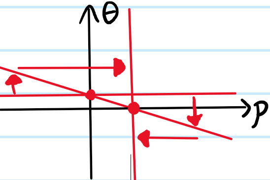
The set of paraxial rays \((\rho,\theta)\) constitute a real, \(2\)-dimensional vector space on which optical elements such as lenses act by linear transformations. For instance, a collection of parallel rays incident on the lens (represented by the horizontal line below) is first sheared vertically by the lens, and subsequently free space propagation by a distance \(f\) shears the resultant line horizontally to the point that it becomes vertical, indicating that all the parallel rays have been focused to the same point (thus, this is an instance of the general identity \(\arctan f+\arctan 1/f=\text{sgn}(f)\pi/2\) for arbitrary \(f\in\textbf R-\{0\}\)).
An important corollary of this is that, if one wishes to observe the Fraunhofer interference pattern of some aperture at any distance \(f\) of interest, not necessarily just in the far-field \(f\gg z_R\), a simple way to achieve this is to just place a thin convex lens of focal length \(f\) into the aperture. Recalling that the Fraunhofer interference pattern arises by the superposition of (essentially) parallel Huygens wavelet contributions from each point on the aperture (parallel because one is working in the far-field), and recalling that a lens focuses all incident parallel rays onto a given point in its back focal plane \(f\), this provides a geometrical optics way of seeing why one can form the Fraunhofer interference pattern at an arbitrary distance \(f\) simply by choosing a suitable convex lens.
There is also a more physical optics way of seeing the same result. Recall that, at the end of the day, a lens is just two spherical caps of radii \(R,R’\) that have been welded together. In Cartesian coordinates, the equations of such caps are \(z=-\sqrt{R^2-x’^2-y’^2}\) and \(z=\sqrt{R’^2-x’^2-y’^2}\), but in the paraxial approximation, these look like the paraboloids \(z\approx -R+(x’^2+y’^2)/2R\) and \(z\approx -R’+(x’^2+y’^2)/2R’\) (where \(R'<0\) for a convex lens, etc.). Here, despite using a “thin” lens approximation, one cannot completely ignore the thickness profile across the lens (also a paraboloid):
\[\Delta z(x’,y’)=R-R’-\frac{x’^2+y’^2}{2}\left(\frac{1}{R}-\frac{1}{R’}\right)\]
So a light ray incident at \((x’,y’)\) on the lens will, upon exiting the lens, have acquired an additional phase shift of:
\[\Delta\phi(x’,y’)=n’k\Delta z(x’,y’)-nk\Delta z(x’,y’)=(n’-n)k\Delta z(x’,y’)\]
It is important to understand that \(k\) here is the free space wavenumber, but that in a medium \(n\) it becomes \(k\mapsto nk\) because \(\omega=ck=vnk\) is fixed. This corresponds to a spatially-varying \(U(1)\) modulation of the aperture field:
\[\psi(x’,y’,0)\mapsto\psi(x’,y’,0)e^{i\Delta\phi(x’,y’)}=\psi(x’,y’,0)e^{i(n’-n)k(R-R’)}e^{-ink(x’^2+y’^2)/2f}\]
where the lensmaker’s equation has been used. But notice that, when inserted into the Fresnel diffraction integral (with \(k\mapsto nk\) and hence \(\lambda\mapsto\lambda/n\)), if one places the screen exactly at \(z=f\), then the quadratic phase terms cancel out and one is left with precisely the Fraunhofer interference pattern:
\[\psi(\textbf x)=\frac{ne^{i(n’-n)k(R-R’)}e^{inkf}e^{ink(|\textbf x|^2-f^2)/2f}}{i\lambda f}\iint_{\textbf x’\in\text{aperture}}\psi(\textbf x’)e^{-in\textbf k\cdot\textbf x’}d^2\textbf x’\]
More generally, for an arbitrary optical component with ray transfer matrix \(\begin{pmatrix}A&B\\C&D\end{pmatrix}\) in the geometrical optics picture, its corresponding operator in the physical optics picture is \(e^{}\).
Problem: Show that \(2\) closely-spaced wavenumbers \(k,k’\) separated by \(\Delta k:=|k-k’|\) can be resolved by a diffraction grating with \(N\) slits at the \(m^{\text{th}}\)-order iff:
\[\frac{\Delta k}{k}\geq \frac{1}{mN}\]
(note the spectral resolution can also be expressed in terms of wavelengths \(\Delta k/k=\Delta\lambda/\lambda\) because \(k\lambda=2\pi\)).
Solution: Although not relevant to the final result, it is useful to introduce the length \(L\) of the entire grating as well as the separation \(d\) between adjacent slits (each considered infinitely thin) so that \(L=Nd\).
Now, for all wavenumbers \(k\), the Fraunhofer interference pattern in \(k_x\)-space looks the same:
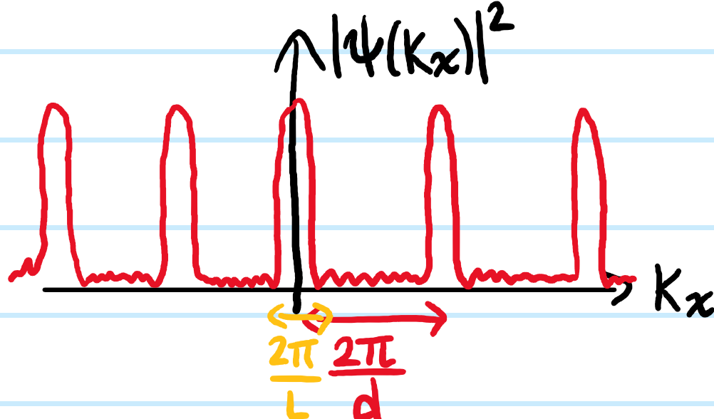

The maxima only appear to split in \(\sin\theta\)-space, where more precisely the \(m^{\text{th}}\)-order maxima of the \(2\) wavenumbers \(k,k’\) are now separated by:
\[\Delta\sin\theta=\frac{2\pi m}{kd}-\frac{2\pi m}{k’d}=\frac{m\Delta\lambda}{d}\]
And the Rayleigh criterion considers these maxima to be resolved iff \(\Delta\sin\theta\) is at least the width (again in \(\sin\theta\)-space) of any one of the maxima \(\frac{2\pi}{kL}=\frac{\lambda}{L}\). So:
\[\frac{m\Delta\lambda}{d}\geq\frac{\lambda}{L}\]
\[\frac{\Delta \lambda}{\lambda}\geq \frac{d}{mL}\]
and finally, just remember \(L=Nd\).
Problem: State the paraxial approximation and show that under this approximation, the envelope amplitude function \(\psi(\mathbf x)\) satisfies the paraxial Helmholtz equation:
\[\frac{\partial^2\psi}{\partial x^2}+\frac{\partial^2\psi}{\partial y^2}+2ik\frac{\partial\psi}{\partial z}=0\]
Solution: The idea is to take the Helmholtz equation \(|\partial/\partial\mathbf x|^2E_0(\mathbf x)=-k^2E_0(\mathbf x)\) and substitute the travelling plane wave ansatz \(E_0(\mathbf x)=\psi(\mathbf x)e^{ikz}\). This gives
\[\biggr|\frac{\partial}{\partial\mathbf x}\biggr|^2\psi+2ik\frac{\partial\psi}{\partial z}=0\]
At this point, the paraxial approximation \(|\partial^2\psi/\partial z^2|\ll |k\partial\psi/\partial z|\) steps in, allowing one to discard the \(\partial^2\psi/\partial z^2\) term in the Laplacian to be left with the transverse Laplacian \(\partial^2\psi/\partial x^2+\partial^2\psi/\partial y^2\) of \(\psi(\mathbf x)\).
Problem: The general solution of the paraxial Helmholtz PDE can be written as a linear combination of so-called Hermite-Gaussian modes, of which the lowest-order \(\text{TEM}_{00}\) mode is a pure Gaussian envelope (which unsurprisingly is the most important mode for e.g. lasers). Show a neat short cut by which one can obtain this solution.
Solution: The idea is to first return to the full Helmholtz equation, for which the outward-propagating spherical wave solution is well-known:
\[E_0(r)\propto\frac{e^{ikr}}{r}\]
The idea is to then write \(r:=\sqrt{\rho^2+z^2}\) and binomial expand this \(r\approx z+\rho^2/2z\) in the paraxial limit \(z\gg\rho\) (at least in the numerator; for the denominator one can just approximate \(r\approx z\)). The resultant \(E_0(r)=\psi(\rho,z)e^{ikz}\) has amplitude \(\psi(\rho,z)\propto e^{ik\rho^2/2z}/z\) satisfying the paraxial Helmholtz equation. However, it is currently not practically useful due to the divergence \(\lim_{z\to 0}\psi(\rho,z)=\infty\) in the \(xy\)-plane. The trick to smooth out this divergence is to recognize the translational invariance of the paraxial Helmholtz equation, i.e. \(\psi(x,y,z)\) is a solution iff \(\psi(x-\Delta x,y-\Delta y,z-\Delta z)\) is a solution for arbitrary \(\Delta x,\Delta y, \Delta z\in\mathbf C\). In particular, in this case a useful origin shift turns out to be \(\Delta x=\Delta y:=0\) and \(\Delta z:=iz_0\) for some positive real number \(z_0>0\) called the Rayleigh range. When this is implemented, one finds the result can be written:
\[\psi(\rho,z)=\frac{\psi(0,0)z_0}{\sqrt{z^2+z_0^2}}e^{-k\rho^2z_0/2(z^2+z_0^2)}e^{ik\rho^2z/2(z^2+z_0^2)}e^{-i\arctan(z/z_0)}\]
or, defining the hyperbolic beam radius profile \(\rho_0^2(z):=(z^2+z_0^2)/2kz_0\) for a Gaussian beam of waist radius \(\rho_0(0)=\sqrt{z_0/2k}\) (conventions here differ; in this convention, the “scattering angle” of the hyperbolic cone in the \(z\gg z_0\) limit is \(2\theta=2\arctan (1/\sqrt{2kz_0})\approx\sqrt{2/kz_0}\)) and radius of curvature \(R(z):=\left(\frac{\partial^2}{\partial\rho^2}\frac{\rho^2z}{2(z^2+z_0^2)}\right)^{-1}=z+z_0^2/z\) of the osculating sphere to the Gaussian beam wavefront a distance \(z\) from the beam waist at \(z=0\):
\[\psi(\rho,z)=\frac{\psi(0,0)\rho_0(0)}{\rho_0(z)}e^{-\rho^2/4\rho^2_{0}(z)}e^{ik\rho^2/2R(z)}e^{-i\arctan(z/z_0)}\]
The corresponding (time-averaged) intensity distribution \(I(\rho,z)\propto |E_0(\rho,z)|^2=|\psi(\rho,z)|^2\) is:
\[I(\rho,z)=I(0,0)\frac{\rho_0^2(0)}{\rho_0^2(z)}e^{-\rho^2/2\rho_0^2(z)}\]
This has the nice property that the total power flow across any plane \(z\in\mathbf R\) is constant \(P=\int_0^{\infty}d\rho 2\pi\rho I(\rho,z)=I(0,0)z_0\lambda/2\).
In practice, if a beam is not perfectly Gaussian, this degree of “non-Gaussianity” can be loosely quantified by measuring the beam’s waist radius \(\tilde{\rho}_0(0)\) and cone semi-angle \(\tilde{\theta}\) and comparing their product with that of a Gaussian beam \(\rho_0(0)\theta=\lambda/4\pi\) via the beam quality:
\[Q^2:=\frac{\tilde{\rho}_0(0)\tilde{\theta}}{\lambda/4\pi}\]
(this is like measuring how “classical” a quantum state is by comparing to a coherent state saturating Heisenberg’s inequality).
Problem: A Gaussian beam of wavenumber \(k\) and Rayleigh range \(z_0\) propagating in the positive \(z\)-direction is incident at a distance \(z>0\) from its waist on a thin lens of focal length \(f\) which phase-modulates the Gaussian beam into a new Gaussian beam of wavenumber \(k’\), Rayleigh range \(z’_0\) whose waist is now at a location \(z'<0\) from the thin lens. How is \(k’,z’_0\) and \(z’\) related to \(k,z_0,z\) and \(f\)? Given the beam waist radius \(\rho_0:=\sqrt{z_0/2k}\) is fixed by \(k\) and \(z_0\), deduce how the beam waist radius transforms \(\rho_0\mapsto\rho’_0\).
Solution: The ray transfer matrix of the thin lens is \(\begin{pmatrix}1&0\\-1/f&1\end{pmatrix}\) which is isomorphic to the Mobius transformation \(q\mapsto q’:=\frac{1q+0}{-q/f+1}=q/(1-q/f)\Rightarrow 1/q’=1/q-1/f\) where \(q(z)=z-iz_0\) and \(q'(z’)=z’-iz’_0\) are the complex beam parameters of the input and output Gaussian beams. Noting that \(1/q(z)=1/R(z)+i/2k\rho_0^2(z)\), one can thus equate real parts \(1/R'(z’)=1/R(z)-1/f\) and imaginary parts \(\rho’_0(z’)=\rho_0(z)\).
Now, \(k’=k\) obviously. However, working out the other parts, it turns out to be convenient to define the magnification \(M(z_0,z,f):=\frac{f}{\sqrt{(z-f)^2+z_0^2}}\), in which terms one has:
\[z’_0=\frac{z_0f^2}{(z-f)^2+z_0^2}\]
\[z’=\frac{f(zf-z^2-z_0^2)}{(z-f)^2+z_0^2}\]
\[\rho’_0=M^2(z_0,z,f)\rho_0\]
- Collimator setup
- Lenses, sign conventions (basically, one key point is that an optical element which tends to converge light rays has positive focal length).
- Real objects are a source of rays, real images are a sink of rays, virtual images are a source of rays (probably all of this can be made precise in the eikonal approximation).
- Gaussian optics as paraxial geometrical optics
- No notion of \(\lambda\) (can view geometrical optics as the \(\lambda\to 0\) limit of physical optics)
- Ray tracing algorithms.
- Spherical aberration
- Chromatic aberration due to optical dispersion \(n(\lambda)\) as the only time where \(\lambda\) shows up, sort of ad hoc.
- Discuss:
- TE/TM/TEM modes in EM waveguides
- How Fresnel diffraction is an exact solution to the paraxial Helmholtz equation