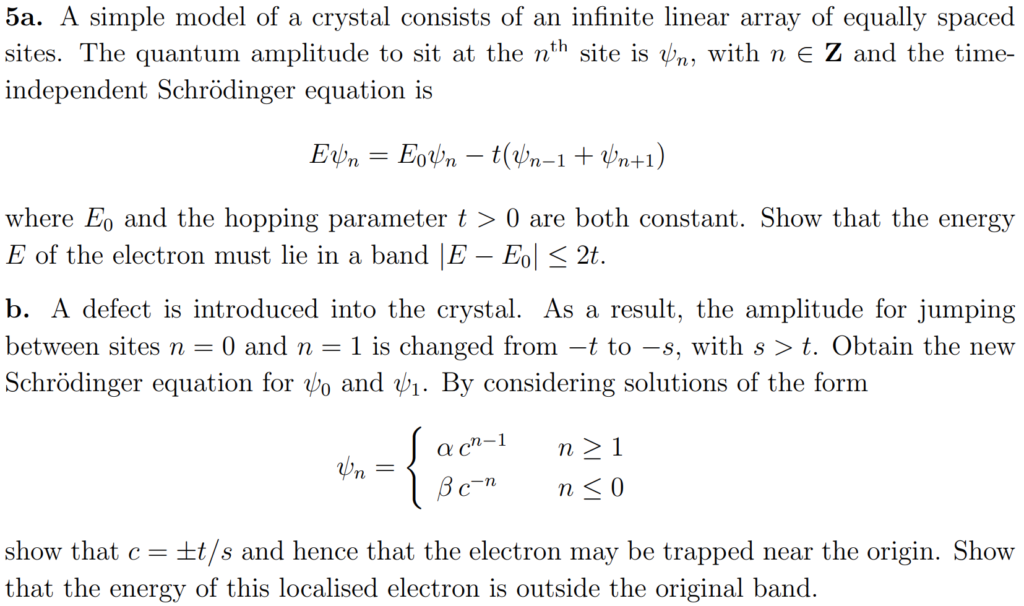
Solution #\(5\): First, although this tight-binding model looks like a classical model, in fact it arises from the quantum Hamiltonian \(H=E_01-t_1\sum_n(|n+1\rangle\langle n|+|n-1\rangle\langle n|)\) together with the “discrete position representation” \(|\psi\rangle=\sum_n\psi_n|n\rangle\Leftrightarrow\psi_n:=\langle n|\psi\rangle\). The piece \(\psi_{n-1}+\psi_{n+1}\) can be coarse-grained to a kinetic energy:
with effective mass \(m^*\) defined through \(\frac{\hbar^2}{2m^*}=t_1\Delta x^2\). The eigenstates are the usual scattering plane waves \(\psi(x)\sim e^{\pm ikx}\) where one has the free particle dispersion relation:
\[E=E_0-2t_1+t_1k^2\Delta x^2\]
This motivates how to proceed, namely replace \(x\mapsto n\Delta x\) and make the ansatz \(\psi_n=e^{ikn\Delta x}\). Doing so gives the cosine band dispersion:
\[E=E_0-2t_1\cos k\Delta x\]
so in this tight-binding approximation there is a single band of width \(4t_1\) centered at \(E_0\) (no notion of band gaps in this model because there’s only \(1\) band!). Notice also that Taylor expanding the \(\cos\) reproduces the earlier free particle dispersion near \(k=0\).
For part b), for \(n\leq -1\) or \(n\geq 2\), in both cases one finds:
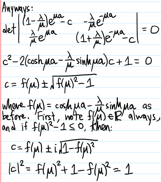
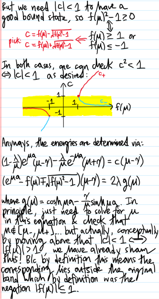
this is a \(2\times 2\) circulant matrix so the (unnormalized) eigenvectors \((\alpha,\beta)=(1,\pm 1)\) are very easy to read off and so no determinant computations are even needed; the dispersion relations are \(E-E_0=-ct_1\pm s\). Eliminating \(E-E_0\) in the “bulk” equation immediately yields \(c=\pm t_1/s\) so that \(|c|<1\) which indicates a bound state in which the electron is localized near the origin by the high-energy \(s>t_1\) defect because \(\psi_n\to 0\) as \(n\to\pm\infty\). The energies \(E_{\pm}=E_0\pm\left(\frac{t_1^2}{s}+s\right)\) may be checked to lie outside the original band \(E\in[E_0-2t_1,E_0+2t_1]\).
And explain why Maxwell relations in general should be viewed as much more than just mathematical identities.
Solution #\(1\): Here it is clear that one is viewing \((T,V)\) as independent variables, and the corresponding energy which has these as its natural variables is the Helmholtz energy \(F\). This has the differential:
All Maxwell relations (for a gas system described by state space \((p,V)\)) can be boiled down to the Jacobian determinant:
\[\frac{\partial (p,V)}{\partial (T,S)}=1\]
which expresses the area/orientation-preserving property of the state space transformation \((p,V)\to(T,S)\). So the point is that thermodynamics is really a theory of geometry (cf. special relativity), the geometry of equilibrium states.
In any Maxwell relation, one partial derivative represents a process which is experimentally accessible, while the other side represents an experimentally difficult quantity to measure (this is typically the entropy \(S\)) but which is in some way seeking to understand microscopic detail. Even to measure (changes in) entropy, one typically measures heat capacities…but the partial derivative is being taken at constant \(T\)! So always write Maxwell relations in a way that agrees with the usual convention in math of putting the dependent variable on the LHS and independent variables on the RHS, in this case putting the experimentally difficult partial derivative on the LHS and the experimentally accessible one on the RHS.
Problem #\(2\): For a gas, what does it mean to have complete thermodynamic information?
Solution #\(2\): Knowing \(N,V,T,\mu,p,S\). For instance, if one specifies a function \(F=F(N,V,T)\) for the Helmholtz energy, then this provides one with complete thermodynamic information since one can obtain \(\mu=\frac{\partial F}{\partial N}, p=-\frac{\partial F}{\partial V},S=-\frac{\partial F}{\partial T}\). Since the Helmholtz free energy is equivalent to giving the canonical partition function \(F=-k_BT\ln Z\), this is unsurprising.
Problem #\(3\): What are the assumptions required for each of the following differential equalities to be true?
\[dE=\bar dQ+\bar dW\]
\[\bar dQ=TdS\]
\[\bar dW=-pdV+\mu dN\]
\[dE=TdS-pdV+\mu dN\]
Solution #\(3\): All \(4\) equations require one to go between \(2\) (infinitesimally separated) equilibrium states. In other words, this is thermodynamics! With this in mind, the first equation is then always trueregardless of the path one takes between those \(2\) equilibrium states (because \(E\) is a state function). However, the \(2^{\text{nd}}\) and \(3^{\text{rd}}\) equations are true iff the path by which one goes between those \(2\) equilibrium states is reversible (since \(\bar dW\) and \(\bar dQ\) are now path functions); if the path were irreversible then both equalities would instead become inequalities! Finally, although at first one may think the \(4^{\text{th}}\) equation is only true for a reversible path, in fact because \(dE\) is an exact \(1\)-form (whereas \(\bar dW,\bar dQ\) are inexact), it is again always true, reversible or irreversible, since at the end of the day all that matters for state functions is the initial and final states.
In the case of \(E\) for a gas, clearly its extensivenatural variables are \(N,V,S\), while its intensive derived variables are \(\mu, p, T\).
This also makes it clearer what the \(1^{\text{st}}\) law of thermodynamics is really saying, i.e. the sum of the inexact \(1\)-forms \(\bar dQ+\bar dW\) is (nontrivially!) an exact \(1\)-form that one happens to call \(dE\). Put another way, it is rooted in a bedrock belief that conservation of energy should hold even in the presence of heat transfer \(\bar dQ\).
Problem #\(4\): What is the difference between a quasistatic and a reversible process?
Solution #\(4\): Reversible processes are a subset of quasistatic processes. More precisely:
Hence, by appealing to extensivity of the energy \(E=E(N,V,S)\), obtain the Gibbs-Duhem relation:
\[SdT-Vdp+Nd\mu=0\]
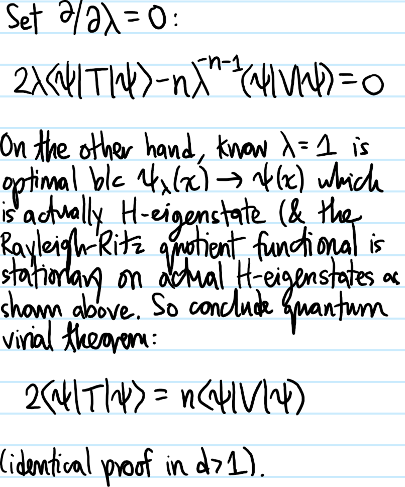
Solution #\(5\): Just differentiate \(\left(\frac{\partial}{\partial\lambda}\right)_{\lambda=1}\) (recognize this as the precursor of the virial theorem!). Extensivity of the energy is equivalent to the \(n=1\) case of Euler’s homogeneous function theorem, i.e.
so because \(dE=TdS-pdV+\mu dN\), the latter part must vanish, which is the Gibbs-Duhem relation.
Problem #\(6\): Using the Gibbs-Duhem relation, prove the Clausius-Clapeyron equation for a single-component system at a \(1^{\text{st}}\)-order phase boundary/coexistence curve:
Solution #\(6\): For each phase of the single-component system, one has a Gibbs-Duhem relation which can be written in the form:
\[S_1dT_1-V_1dp_1+N_1d\mu_1=0\]
\[S_2dT_2-V_2dp_2+N_2d\mu_2=0\]
Now, the defining property of a phase boundary is that the \(2\) phases are in equilibrium, so the intensive variables between the \(2\) phases are equal everywhere on the phase boundary \(T_1=T_2:=T,p_1=p_2:=p,\mu_1=\mu_2:=\mu\). So moving infinitesimally along this phase boundary, it is a rigorous corollary that \(dT_1=dT_2:=dT,dp_1=dp_2:=dp,d\mu_1=d\mu_2:=d\mu\). But now one has \(2\) equations and \(3\) unknowns \(dT,dp,d\mu\):
\[S_1dT-V_1dp+N_1d\mu=0\]
\[S_2dT-V_2dp+N_2d\mu=0\]
Eliminating \(d\mu\) yields the Clausius-Clapeyron equation:
Or in terms of molar entropies \(s:=S/n\) and molar volumes \(v:=V/n\), where \(n:=N/N_A\):
\[\frac{dp}{dT}=\frac{\Delta s}{\Delta v}\]
So in other words, phase transitions are all about parameters changing discontinuously, and in this case the discontinuous changes \(\Delta s,\Delta v\) are directly also what influence the slope of the phase boundary.
Because the phase transition occurs isothermally at temperature \(T\), one can also write \(\Delta s:=q_L/T\) where \(q_L\) is the molar latent heat released during the phase transition. And often, if it’s a liquid-to-gas phase transition, the molar volume of liquid water \(v_{\ell}\approx\) is significantly less than the molar volume of water vapor \(v_{\text H_2\text O(\text g)}\approx\), so it is common to approximate \(\Delta v\approx v_g\approx RT/p\) (if the gas is ideal) so that \(q_L\) refers to the specific latent heat of vaporization \(\ell\to\text g\) and, assuming \(q_L\) to be approximately \(T\)-independent, the Clausius-Clapeyron equation can be integrated to yield the equation of the phase boundary itself:
shows that \(q_L\) can be experimentally determined through linear regression of \(\ln p\) vs. \(1/T\).
Finally, note that earlier the choice was made to eliminate \(d\mu\) to isolate for \(dp/dT\); however one could just as well have eliminated \(dp\) to isolate for \(d\mu/dT\) or eliminated \(dT\) to obtain \(dp/d\mu\)…each giving rise to its own kind of Clausius-Clapeyron equation.
Problem #\(7\): Using the fact that in a closed cycle \(\oint dE=0\), write \(dE=TdS-pdV+\mu dN\) and apply Stokes’ theorem to obtain suitable Maxwell relations.
Solution #\(7\): Stokes’ theorem needs a curve and a surface with that as its boundary curve. First, consider looking at just motion in the \((S,V)\)-plane so that \(dN=0\). Then Stokes’ theorem reduces to Green’s theorem in that plane:
Working in the \((N,S)\) plane or \((N,V)\) plane produces \(2\) other Maxwell relations.
Problem #\(8\): Equation of state as a constitutive relation/dispersion relation/heart of the physics. Want to distinguish clearly between this and all the kinematic Maxwell relations, definitions, etc.
Equations of state will never involve entropy \(S\), the experimentally inaccessible bastard. So when one encounters any \(\partial S\) quantities, the immediate knee-jerk reaction should be to convert it to a corresponding \(\partial T\) derivative which is more readily measurable.
All the usual shorthands for special collections of partial derivatives like heat capacities, thermal expansion coefficients, compressibilities/bulk moduli, and other moduli are singled out for this special treatment because they are often found to be constant material parameters?
Problem: In general, the energy may be written abstractly as a linear combination of \(N\) extensive natural variables \(Q_i\) (thought of as “generalized charges/coordinates“) weighted by their \(N\) conjugateintensivederived variables \(\phi_i\) (thought of as “generalized potentials/forces“):
\[E=\sum_{i=1}^N\phi_iQ_i\]
For instance, temperature \(T\) can be thought of as an “entropy potential” as entropy \(S\) flows via heat from high \(T\) to low \(T\). Similarly, \(\sigma=-p\) is a “volume potential”, thus volume \(V\) flows from high \(\sigma\) to low \(\sigma\), aka from low \(p\) to high \(p\) (this is consistent with the usual interpretation of pressure \(p\) as a force acting on the piston walls). Similarly, particles \(N\) flow from high chemical potential \(\mu\) to low \(\mu\). In general, charge \(Q_i\) flows from high potential \(\phi_i\) to low \(\phi_i\).
How many Maxwell relations can be obtained from \(E\) alone and what is their general form?
Solution: There are \(N\choose{2}\)\(=\frac{N(N-1)}{2}\) Maxwell relations that can be wringed out from this equilibrium potential \(E\) alone. Because there are no fiddly minus signs in this series, it is clear that there won’t be any fiddly minus signs in the corresponding Maxwell relations. In this case, all Maxwell relations will have the form:
Problem: For a closed single-component \(3\)D gas in equilibrium, how many independent intensive variables parameterize the equilibrium manifold of the system?
Solution: The Gibbs phase rule (analogous to Euler’s graph formula \(F+V=E+2\)) asserts:
\[I+P=C+2\Rightarrow I+1=1+2\Rightarrow I=2\]
So one is always free to select any \(2\) intensive potentials such that when their values are fixed, so too automatically are the values of all other intensive potentials at equilibrium. It’s a bit like saying if a mass is acted on by forces \(\textbf F_1,\textbf F_2,\textbf F_3\), and one is told \(\textbf F_1,\textbf F_2\), then because the mass is in translational equilibrium the value of \(\textbf F_3=-\textbf F_1-\textbf F_2\) is fixed.
Problem: For a single-component \(3\)D gas with energy/Hamiltonian:
\[E=TS+\sigma V+\mu N\]
Explain whether the following partial derivatives are (in general) well-posed or not. For those that are well-posed, write down their associated Maxwell relation.
Solution: It is useful to define the notion of a natural variable set to be any energy together with its set of natural variables which are the natural variables of some energy. Starting from the fundamental natural variable set:
\[\{E,S,V,N\}\]
Legendre transforms give all \(8\) of the other natural variable sets:
\[\{F,T,V,N\}\]
\[\{H,S,\sigma,N\}\]
\[\{G,T,\sigma,N\}\]
\[\{\Phi,T,V,\mu\}\]
and \(3\) other combinations that don’t seem to have a name. Anyways, the point is that the Gibbs phase rule gives \(I=2\), but it doesn’t count the extensivity degree of freedom which is always present because that doesn’t affect equilibrium, hence explaining why all natural variable sets have \(2+1=3\) variables. Moreover, as should be clear from the fact that one is Legendre transforming, no variable appears with its conjugate in the same natural variable set.
This then provides a litmus test for whether a partial derivative is ill-posed or not; just see if the variables in the subscript together with either the variable in the numerator or the variable in the denominator can be made to form a natural variable set or not; more simply, can one form a set which is not cohabited by conjugate variables (is there a notion of conjugate variables for the energies like \(E,F,\)etc, themselves that makes the Maxwell relations continue to hold)?
(aside: actually this last partial derivative should be undefined? because holding both \(\sigma,\mu\) constant amounts to holding \(T\) constant since they’re intensive…?)
Also, given any \(2\) extensives \(E_1,E_2\) and any \(2\) distinct intensives \(I_1\neq I_2\), the partial derivative:
this follows because \(E_1/E_2\) is intensive so equal to a constant \(\lambda=\lambda(I_1,I_2)\), so \(E_1=\lambda E_2\Rightarrow \partial E_1/\partial E_2=\lambda=E_1/E_2\).
Aside: when intensive and intensive or extensive and extensive bunch together like bosons, then the Maxwell relation has a minus sign. Similarly, intensive and extensive antibunch like fermions but that gives a + sign Maxwell relation. It seems that, roughly speaking, the individual intensive/extensive variables can treated like fermions, in the sense that starting with any Maxwell relation and exchanging \(\phi_i\Leftrightarrow Q_i\) gives a minus sign. And obviously equality is symmetric which is really a reflection of the fact that 2 fermions together make a boson.
Problem: For a single-component system, what are the \(3\) standard intensive equilibrium material properties?
Solution: The compressibility (either the isothermal one \(\kappa_T\) or the isentropic one \(\kappa_S\), and equivalently one can use the isothermal bulk modulus \(B_T\) or the isentropic bulk modulus \(B_S\)), the specific heat capacity (either \(c_V\) or \(c_p\) and note it could be per unit mass or per unit mole, etc.) and the thermal expansion coefficient \(\alpha\). The definitions are here.
Problem: Using the compressible Bernoulli’s equation, show that enthalpy is conserved in a Joule-Thomson expansion. Define the corresponding Joule-Thomson coefficient \(\mu_{\text{JT}}\) and show that \(\mu_{\text{JT}}=0\) for ordinary Joule expansion of an ideal gas.
Solution: The compressible Bernoulli equation looks like the usual Bernoulli equation but with the addition of the gas’s specific energy \(e\):
The terms \(h:=e+p\) are nothing more than the specific enthalpy of the gas.
In Joule-Thomson expansion, it is conventional to assume the macroscopic energy density \(\frac{1}{2}\rho v^2+\rho\phi\) is constant throughout the expansion, so this implies that \(h\) is conserved.
Alternatively, one can imagine a setup in which gas at a higher (but constant) pressure \(p\) is throttled through a porous plug to a region of lower (constant) pressure \(p'<p\). Then, the gas behind does work \(pV\) on the gas that passes through, and similarly the gas that expands in the other side does work \(p’V\) on the gas in front of it (too lazy to draw this). It’s as if there were fictitious pistons on either side of the plug…assuming the whole thing is enclosed in adiabatic walls, so \(Q=0\), then from the first law of thermodynamics, \(\Delta H=0\).
The Joule-Thomson temperature change \(\Delta T_{\text{JT}}\) is familiar in everyday life. For instance, when opening a bike tire valve, the pressure inside is initially a few atmospheres higher than the ambient atmospheric pressure, but as the gas escapes (isenthalpically) it cools down, causing the tire valve to feel cold to the touch. Physically, for a non-ideal gas, expansion increases potential energy, reducing kinetic energy, hence cooling the gas.
quantifies this cooling across a pressure differential (for most gases at room temperature, the Joule-Thomson coefficient is positive and of order \(\mu_{\text{JT}}\sim 0.1\frac{\text J}{\text{atm}}\), hence explaining the cooling rather than heating normally observed).
For an ideal gas, \(\alpha=1/T\) so there is no associated Joule-Thomson cooling/heating across a pressure differential. The inversion point is when \(\mu_{\text{JT}}=0\).
Problem: Distinguish between heat engines, refrigerators, and heat pumps.
Solution: A heat engine \(\textbf x_E(t)\) is an abstraction of any periodic process \(\textbf x_E(t+\Delta t)=\textbf x_E(t)\) whose net outcome in each period \(\Delta t\) is to convert some amount of (useless!) heat \(Q_H>0\) into (useful!) work \(W>0\) (thus, both \(Q_H\) and \(W\) are normalized per orbit of the heat engine \(\textbf x_E(t)\) in a suitable state space). It thus makes sense to define the efficiency \(\eta\) of a heat engine by the buck-to-bang ratio:
\[\eta:=\frac{W}{Q_H}\]
Kelvin’s formulation of the \(2^{\text{nd}}\) law of thermodynamics is logically equivalent to the assertion that the efficiency \(\eta\) of any heat engine \(\textbf x_E(t)\) must obey:
\[\eta<1\]
though in theory \(\eta\) can get arbitrarily close to \(1\). Schematically, for each orbit:
Since \(E\) is a function of the engine’s state \(\textbf x_E(t)\) only, over each \(\Delta t\)-orbit, \(\oint dE=0\) so the first law of thermodynamics guarantees \(\oint\bar dQ+\oint\bar dW=0\). This guarantees that \(Q_H=W+Q_C\) over each engine period \(\Delta t\).
Both refrigerators and heat pumps are basically the same thing (note: refrigerators are not called “heat refrigerators” even though that would have been more consistent with “heat engine” and “heat pump”). They are also both abstractions of any periodic process whose net outcome in each period is to remove some amount of heat \(Q_C>0\) from a colder place and dump some of that heat \(Q_H>0\) into a hotter place, fighting an uphill battle against the spontaneous direction that heat would otherwise flow (i.e. from hotter to colder). The difference between refrigerators and heat pumps is simply a matter of emphasis; in the case of refrigerators, the goal is to remove as much heat \(Q_C\) from the cold place as possible, whereas for heat pumps the goal is to dump as much heat \(Q_H\) into the hot place as possible. Schematically, for each orbit:
Clausius’s formulation of the \(2^{\text{nd}}\) law of thermodynamics is logically equivalent to the assertion that for any refrigerator or heat pump, \(Q_H<Q_C\). This implies that some external work \(W>0\) must be done each cycle to facilitate this heat transfer. This motivates the corresponding definitions of the coefficient of performance \(\text{COP}\) for a refrigerator:
\[\text{COP}:=\frac{Q_C}{W}\]
and a heat pump:
\[\text{COP}:=\frac{Q_H}{W}\]
Problem: Explain what the reversibility theorem (also misleadingly called “Carnot’s theorem”) asserts.
Solution: The notions of heat engines and refrigerators/heat pumps are very general, and a priori there is no requirement about “using a hot reservoir \(T_H\) and a cold reservoir \(T_C\)”. However, if one restricts one’s scope to just the subset of heat engines and refrigerators/heat pumps operating only between \(2\) heat reservoirs \(T_H,T_C\), then within this subset one can prove that reversible cycles are the most efficient in all cases (i.e. for heat engines they maximize \(\eta\), and for refrigerators/heat pumps they maximize \(\text{COP}\)).
Problem: Show that the specific example of a Carnot cycle is reversible (though it certainly isn’t the only reversible cycle one can take), and hence compute \(\eta\) for a Carnot heat engine and \(\text{COP}\) for both a Carnot refrigerator and a Carnot heat pump, thus obtaining upper bounds on these values within the subsets described earlier.
Solution: The key is that every step of the Carnot cycle is reversible, regardless of whether it is run as a heat engine or as a refrigerator/heat pump. The universal way to depict the Carnot cycle is on the \((T,S)\)-plane:
Any other depiction of the Carnot cycle, such as in the \((p,V)\)-plane using an ideal gas working substance is then simply a geometric deformation of this rectangle:
For a Carnot heat engine, the efficiency is:
\[\eta=1-\frac{T_C}{T_H}<1\]
For a Carnot refrigerator, the coefficient of performance is:
\[\text{COP}=\frac{T_C}{T_H-T_C}\]
And for a Carnot heat pump:
\[\text{COP}=\frac{T_H}{T_H-T_C}\]
Problem: By a Stokes-like maneuver, any reversible cycle can be decomposed into a bunch of Carnot “vortices” (more precisely, isothermal and adiabatic segments). Hence, establish the Clausius inequality:
\[\oint\frac{\overline{d}Q}{T}\leq 0\]
with equality if and only if the cycle is reversible (e.g. a Carnot cycle).
Solution:
The fact that \(\oint\frac{\overline{d}Q}{T}=0\) in the space of reversible cycles implies that there exists a conservative field \(S\) called the entropy that only depends on the initial and final equilibrium states.
Now suppose that first electron \(e^-\) naturally “burrows” its way down to the ground state \(\textbf n=\textbf k=\textbf 0\) in order to minimize its energy \(E=0\). Now put a second electron \(e^-\) into the box. In reality, the two electrons \(e^-\) would by their mutual Coulomb repulsion run away from each other on a hyperbolic orbit so to speak, raising all energy levels \(E_{\textbf n}\). However, for now we shall ignore all interactions. Then basically we have right now an ideal electron gas of two \(e^-\) that don’t talk to each other. However, actually there is one fundamental quantum mechanical “interaction” so to speak between the two \(e^-\) that cannot be ignored; this is the Pauli exclusion interaction arising from the identical fermionic nature of the spin \(s=1/2\) electrons \(e^-\). Here, as typical, we incorporate spin in an ad hoc manner as just another good quantum number whose associated operators \(\textbf S^2,S_3\) commute with the free space Hamiltonian \(H=T\) of the box. So if the first electron \(e^-\) is in state \(|\textbf n=\textbf 0\rangle\otimes|\uparrow\rangle\), then the second electron \(e^-\), if it also wants to minimize its energy, would have to occupy the state \(|\textbf n=\textbf 0\rangle\otimes|\downarrow\rangle\) (so the total state of the \(2\)-body electron system would be \(|\textbf n=\textbf 0\rangle\otimes|\textbf n=\textbf 0\rangle\otimes\frac{1}{\sqrt 2}(|\uparrow\rangle\otimes|\downarrow\rangle-|\downarrow\rangle\otimes|\uparrow\rangle)\)). The third electron \(e^-\) would then have to live in state \(|\textbf n=(1,0,0)\rangle\otimes|\uparrow\rangle\) for instance and in general we can house \(2\Omega(E_{(1,0,0)})=12\) electrons \(e^-\) in the next energy level, and so forth according to the non-zero values of the scatter plot above. In particular, if one puts in \(N\sim 10^{23}\) electrons for this ideal free electron gas, one would basically fill up a (discrete) ball of electrons in \(\textbf k\)-space (called the Fermi sea) of some radius \(k_F\approx\left(\frac{3N}{8\pi}\right)^{1/3}\), with each lattice point holding two electrons of opposite spin. The spherical boundary \(S^2\) of the Fermi sea of the ideal free electron gas would be called its Fermi surface, whose states thus have momentum \(\hbar k_F\) (called the Fermi momentum) and energy \(E_F=\frac{\hbar^2k_F^2}{2m}\) (called the Fermi energy).
Metals vs. Insulators
In practice, we’re not interested in an empty lattice \(\Lambda=\emptyset\), but rather a non-empty lattice \(\Lambda\neq\emptyset\) such as an atomic lattice in a solid! And what’s more, electrons \(e^-\) don’t just “get added” by some external agent, but rather emerge naturally as the valence electrons \(\partial e^-\) from the atoms located at the lattice sites \(\textbf x\in\Lambda\); thus, working inside a solid kills both birds with one stone.
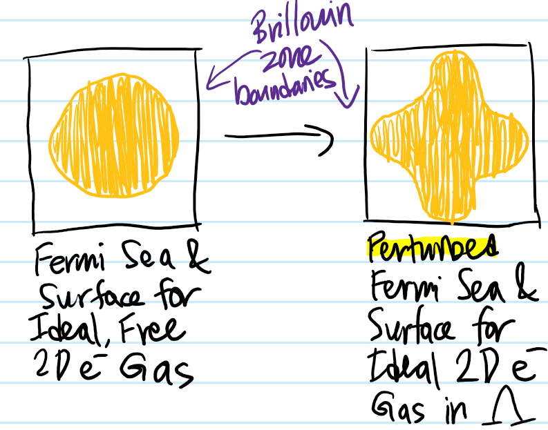
At a high level, the act of superimposing a Bravais lattice \(\Lambda\) within what used to be an empty cube of sides \(L\) can be treated perturbatively exactly as one does in the nearly free electron model. Specifically, we’re still keeping the ideality/non-interacting assumption between the electrons (with the caveat of the Pauli interaction already mentioned), but now we go from being free\(\rightarrow\)nearly free (used in a technical sense). From that analysis, we know that the presence of the \(\Lambda\)-periodic potential butchers the previous free electron dispersion relation \(E(\textbf k)=\hbar^2|\textbf k|^2/2m\) into an energy band structure \(E_{\text{bands}}(\textbf k)\) where each Brillouin zone \(\Gamma_{\Lambda^*}^{(0)},\Gamma_{\Lambda^*}^{(1)}\), etc. (or bijectively, each energy band \(E_{\text{bands}}(\Gamma_{\Lambda^*}^{(0)}),E_{\text{bands}}(\Gamma_{\Lambda^*}^{(1)})\)) can accommodate precisely \(N\) momentum \(\textbf k\)-states (and thus \(2N\) electrons \(e^-\)) where \(N\) is the number of atoms in the solid. Suppose each atom contributes \(Z\) valence electrons (called its valency). Then the total number of free electrons roaming the solid will be \(ZN\), corresponding to the occupation of \(Z/2\) Brillouin zones or equivalently energy bands. In the ideal free electron case, we saw that the Fermi sea was a ball and its Fermi surface boundary \(\partial=S^2\) a sphere. Now, in the ideal nearly free electron case, we know that the energy is lowered at the boundary \(\partial\Gamma_{\Lambda^*}\) of the Brillouin zones (viewed from “within” otherwise how would the energy band gap form?) so this will distort the Fermi sea (and by extension the Fermi surface \(E_F\)-“equipotential”) of electrons towards it (but conserving in this case the area or in \(3\)D the volume of the Fermi sea since that’s the number of occupied \(\textbf P\)-eigenstates). For \(Z=1\) alkali metal solids or other metals (e.g. \(\text{Li},\text{Cu}\)), the act of “turning” on the perturbation due to the presence of the lattice \(\Lambda\) would look (for a \(2D\) material) something like (because \(Z=1\), the area of the initial Fermi sea/disk must be half the area of the square Brillouin zone):
It is clear in this \(2\)-dimensional case that, if the potential \(V\) induces a sufficiently large energy band gap (as it turns out it does for \(\text{Cu}\)), the Fermi surface can cross the Brillouin zone boundary \(\partial\Gamma_{\Lambda^*}\), though it must do so orthogonally in the reduced scheme to maintain its smoothness by virtue of the toroidal topology \(\Gamma_{\Lambda^*}\cong S^1\times S^1\) of the Brillouin zone.
Now, why do we care about the Fermi surface so much? Short answer: because materials with Fermi surfaces are metals. Qualitatively, the idea is that only the electrons with momentum \(\textbf k\) living on the Fermi surface of the system can actually do anything (having access to a bunch of unoccupied states slightly higher in energy to be able to respond to e.g. an \(\textbf E_{\text{ext}}\) to minimize their energy and form a current \(\textbf J=\sigma\textbf E_{\text{ext}}\)) just as only the valence electrons \(\partial e^-\) could delocalize (except that the former is a “meta-layer” of valency above the latter!). Any electrons \(e^-\) deep in the Fermi sea are pretty much trapped there by the Pauli exclusion principle since there’s no room for them to climb up into nearby energy levels above because they’re already occupied by other electrons (it would take a lot of energy for them to escape)!
For a sense of scale, most metals typically have Fermi temperatures on the order of \(T_F=E_F/k\sim 10^4\text{ K}\) (which is about twice as hot as the surface of the Sun \(\odot\)). This is why Fermi surfaces are also strictly defined at absolute zero \(T=0\), since most real materials in room temperature environments are nowhere near their Fermi temperature \(T_F\).
Another point is that, of course, the number of low-energy excitations available in a metal is proportional to the surface area \(\sim k_F^2\sim E_F\) of its Fermi surface (because each point on the Fermi surface corresponds to an excitable electron \(e^-\)).
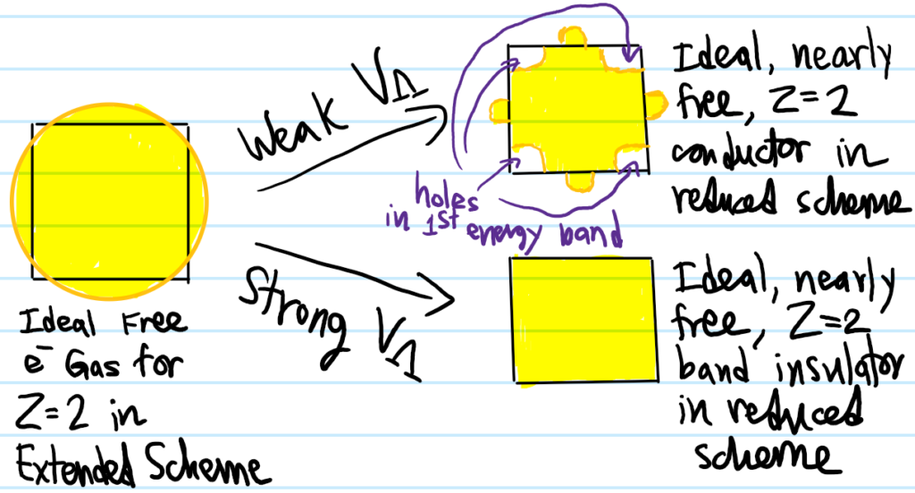
Now consider \(Z=2\) atoms (e.g. alkaline earth atoms like \(\text{Be}\)). Now the initial Fermi sea/disk for the ideal free electron system has area equal to the square, but geometrically this implies that it must leak out the boundary of the Brillouin zone a little bit. If one now superimposes the perturbing lattice \(\Lambda\), there are \(2\) possibilities depending on the strength of the periodic lattice potential \(V_{\Lambda}\):
One might think the Fermi surface in the case of band insulators is just the boundary \(\partial\Gamma_{\Lambda^*}\) of the Brillouin zone but that’s not right because it’s not an equipotential with respect to any well-defined Fermi energy \(E_F\).
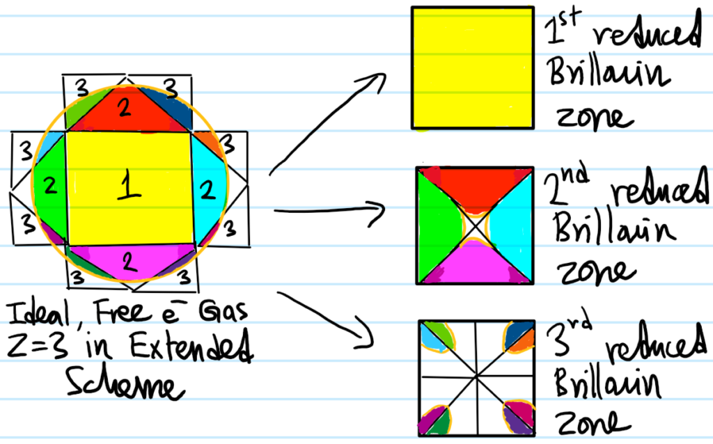
From here onwards \(Z=3,4,5,…\), the qualitative classification essentially repeats. Metals for instance may have several fully-occupied core bands, a fully-occupied valence band, and then right above that a partially-occupied conduction band. Note though that the Fermi surface need not lie solely in a single Brillouin zone, but can have sections distributed through several Brillouin zones. For example, if we consider the ideal, free electron gas with \(Z=3\) this time (so the area of the circle is three times that of the square \(1\)-st Brillouin zone that it now contains), then:
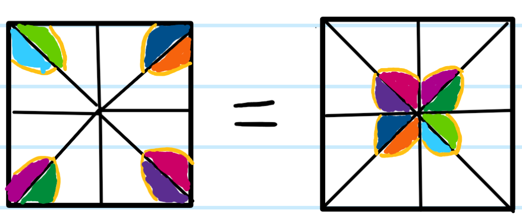
Although the Fermi surface in the \(3\)-rd Brillouin zone square looks disconnected, in fact it is connected (as it was in the extended scheme) because opposite sides of that square in the reduced scheme are topologically glued together (put another way, within the \(3\)-rd Brillouin zone reduced square, if one shifts the “origin” from where it is right now to the top right corner for instance (although all corners are equivalent), then the Fermi surface clearly becomes connected (see this either by tessellating the square or thinking of it as a torus \(S^1\times S^1\) and wrapping the square on itself):
This concludes a qualitative overview of band theory (classification of materials based on whether they are gapped or gapless). While the framework in general is fairly robust, there are some situations where its predictions fail. And as one might suspect, the origin of such deviations are due to one of the assumptions of band theory not being satisfied, notably the assumption of ideality. Examples of these deviations include semiconductors, Mott insulators (cf. band insulators), and topological insulators.
The purpose of this post is to calculate the energy band structure of the famous \(2\)-D material graphene. This of course is a monolayer of carbon \(\text C\) atoms arranged in a hexagonal “honeycomb” lattice. Sheets of graphene stacked on each other are called graphite.
Triangular Lattices, Brillouin Zone, Dirac Points
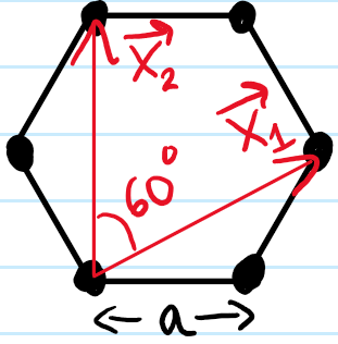
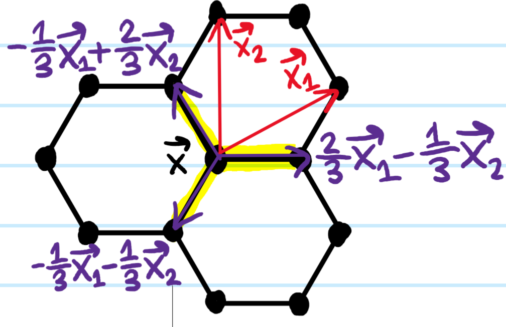
The first thing to notice is that this hexagonal lattice is non-Bravais because the \(\text C\) atoms are not in identical environments. As usual, this is resolved by viewing it as the convolution of a Bravais triangular lattice \(\Lambda_{\Delta}\) with a motif of \(2\)-carbon atoms dropped at each lattice point of \(\Lambda_{\Delta}\) (strictly speaking, this \(\Lambda_{\Delta}\) that I’m calling “triangular” is also confusingly often called hexagonal in crystallography). Therefore, we use the following primitive lattice vectors \(\textbf x_1,\textbf x_2\) which \(\text{span}_{\textbf Z}(\textbf x_1,\textbf x_2)=\Lambda_{\Delta}\):
Note that the lengths of the primitive lattice vectors are related to the inter-carbon atom spacing \(a\approx 1.4\) Å by \(|\textbf x_1|=|\textbf x_2|=\sqrt 3a\) and that the area of the spanning parallelogram is \(|\textbf x_1\times\textbf x_2|=\frac{3\sqrt{3}}{2}a^2\). Of course we also have a reciprocal Bravais lattice \(\Lambda^*_{\Delta}\) which is also triangular and spanned by reciprocal lattice vectors \(\textbf k_1,\textbf k_2\in\Lambda^*_{\Delta}\):
where now \(|\textbf k_1|=|\textbf k_2|=\frac{4\pi}{3a}\) and \(|\textbf k_1\times\textbf k_2|=\frac{8\pi^2}{3\sqrt{3}a^2}\) by the defining criterion \(\textbf x_{\mu}\cdot\textbf k_{\nu}=2\pi\delta_{\mu\nu}\). The first Brillouin zone is hexagonal and henceforth we reduce all other Brillouin zones to this:
where the side lengths of the Brillouin zone hexagon are \(\frac{4\pi}{3\sqrt{3}a}\) and thus the area of the Brillouin zone is \(\frac{8\sqrt 3\pi^2}{a^2}\). It turns out for graphene that the corners of the Brillouin zone hexagon are especially interesting points, called the Dirac points \(\textbf k_{\text{Dirac}}^{\pm}\) of graphene. Despite the fact that the Brillouin zone hexagon has \(6\) vertices, there are only really \(2\) physically distinct Dirac points as labelled because the other Dirac points are manifestly connected to them by a reciprocal lattice vector in \(\text{span}_{\textbf Z}(\textbf k_1,\textbf k_2)=\Lambda^*_{\Delta}\) and so are identified modulo the reduced zone scheme.
Physics of Graphene (Tight-Binding)
Each carbon \(\text C\) atom in graphene has valence \(Z=1\) from donating its one \(2p_3\) atomic orbital electron \(e^-\) into a collective \(\pi\) orbital delocalized over the entire graphene sheet. We’ll model these electrons as being tightly bound to carbon \(\text C\) atoms but free to tunnel/hop around the graphene lattice. In general, the tight-binding/hopping Hamiltonian is:
where \(\mathcal M\) is the \(2\)-carbon atom motif at each lattice point in \(\Lambda_{\Delta}\), \(t_n\in\textbf R\) are hopping energy amplitudes for \(n\)-th nearest neighbours, \(|\textbf x’\rangle\langle\textbf x|=(|\textbf x\rangle\langle\textbf x’|)^{\dagger}\) are mutual adjoints which physically permits bidirectional tunneling and mathematically ensures \(H^{\dagger}=H\) is Hermitian, and \(|\textbf x-\textbf x’|_1\) is a taxicab-like metric on the triangular Bravais lattice \(\Lambda_{\Delta}\) which makes it into a metric space, defined as the shortest number of hops between the two points \(\textbf x,\textbf x’\in\Lambda_{\Delta}\) (in graph theoretic terms, this is commonly called the graph geodesic distance between \(\textbf x\) and \(\textbf x’\)). In practice, it is common to restrict to only \(n=0\) (the on-site energy) and \(n=1\) (nearest neighbour) hopping, thereby ignoring all hopping across \(n\geq 2\) atoms. For graphene, the nearest-neighbour hopping energy amplitude turns out to be \(t_1\approx 2.8\text{ eV}\). With this simplification, the tight-binding Hamiltonian becomes (via a resolution of the identity):
Since the \(n=0\) term \(-2t_01\) is just proportional to the identity \(1\), it doesn’t affect any of the physics so we can ignore it henceforth. For graphene, there are of course \(3\) nearest neighbour carbon atoms \(\textbf x’\in\Lambda_{\Delta}*\mathcal M\) for each carbon atom at position \(\textbf x\in\Lambda_{\Delta}\):
As usual, we now declare that we wish to solve \(H|E\rangle=E|E\rangle\). For this we’ll simply make a Wannier-type ansatz of the \(H\)-eigenstate \(|E\rangle\) as a sum of plane waves modulated by
The purpose of this post is to discuss historically one of the first decision problems for which quantum computing was shown to provide an exponential advantage over classical computing. One of the initially striking discrepancies between classical logic gates such as \(\text{AND}\) and quantum logic gates \(\Gamma\in U\left(\textbf C^{2^N}\right)\) is that the former need not be invertible or reversible (though they can be like the \(\text{NOT}\) gate) whereas the latter are always invertible being unitary \(\Gamma^{-1}=\Gamma^{\dagger}\). However, this is a bit of an illusion. Actually, given any classical logic gate \(\Gamma:\{0,1\}^n\to\{0,1\}^m\) mapping input \(n\)-bit strings to output \(m\)-bit strings (also called Boolean vector-valued functions), it is possible to construct a reversible classical logic gate \(\tilde{\Gamma}:\{0,1\}^{n+m}\to\{0,1\}^{n+m}\) defined as follows:
A qubit is any quantum system with a two-dimensional state space \(\mathcal H\cong\textbf C^2\). In particular because the state space is two-dimensional \(\dim\textbf C^2=2\), the Gram-Schmidt orthogonalization algorithm guarantees the existence of an orthonormal basis \(|0\rangle,|1\rangle\in\mathcal H\) of state vectors spanning \(\text{span}_{\textbf C}|0\rangle,|1\rangle=\mathcal H\) the entire state space \(\mathcal H\) of the qubit. For a larger system of \(N\in\textbf Z^+\) qubits, the corresponding state space \(\mathcal H_N\) is the \(N\)-fold tensor product \(\mathcal H_N\cong\left(\textbf C^2\right)^{\otimes N}\cong\textbf C^{2^N}\) of each qubit’s individual two-dimensional state space, with the dimension \(\dim\mathcal H_N\) of this composite Hilbert space \(\mathcal H_N\) growing exponentially \(\dim\mathcal H_N=2^N\) in the number \(N\) of qubits.
Bloch Sphere Representation of Physical Qubit States
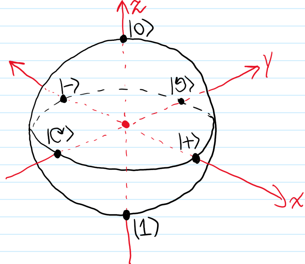
One useful way to visualize physical qubit states \(|\psi\rangle\in P(\textbf C^2)\) (of an individual qubit) is via the Bloch sphere. The idea is to think of the qubit as being concretely realized by the spin angular momentum degree of freedom of a spin \(s=1/2\) isolated electron \(e^-\) whose position is fixed in an inertial frame in \(\textbf R^3\). Suppose one were to then make a measurement (e.g. with a suitable Stern-Gerlach filter) of the electron’s spin angular momentum \(\textbf S\) along some arbitrary direction \(\hat{\textbf n}\in S^2\) of one’s liking given in spherical coordinates by \(\hat{\textbf n}=\cos\phi\sin\theta\hat{\textbf i}+\sin\phi\sin\theta\hat{\textbf j}+\cos\theta\hat{\textbf k}\). Then for spin \(s=1/2\) quantum particles, there are precisely two possible (though not necessarily equiprobable) outcomes of such a measurement, namely \(m_s=\pm 1/2\) corresponding to an electron \(e^-\) either “spinning” aligned or anti-aligned with the direction \(\hat{\textbf n}\) of measurement. In particular, the electron’s spin state then collapses non-unitarily to the corresponding \(\hat{\textbf n}\cdot\textbf S\)-eigenstate which one can check are given by \(|m_s=1/2\rangle=\cos(\theta/2)|0\rangle+e^{i\phi}\sin(\theta/2)|1\rangle\) and \(|m_s=-1/2\rangle=-e^{-i\phi}\sin(\theta/2)|0\rangle+\cos(\theta/2)|1\rangle\) where \(|0\rangle,|1\rangle\) is the \(S_3\)-eigenbasis. In particular, the \(\hat{\textbf n}\)-aligned spin angular momentum eigenstate \(|m_s=1/2\rangle\) of \(\hat{\textbf n}\cdot\textbf S\) provides a general parameterization of an arbitrary electron spin state in \(\textbf C^2\) simply because the electron \(e^-\) has to be “spinning” along some direction \(\hat{\textbf n}\in S^2\) at all times (of course the same is true of the \(\hat{\textbf n}\)-antialigned spin angular momentum eigenstate \(|m_s=-1/2\rangle\), but it’s just more intuitive to work with the former). The map \(|m_s=1/2\rangle\mapsto\hat{\textbf n}\) is then the essence of the Bloch sphere \(S^2\) representation of physical qubit states.
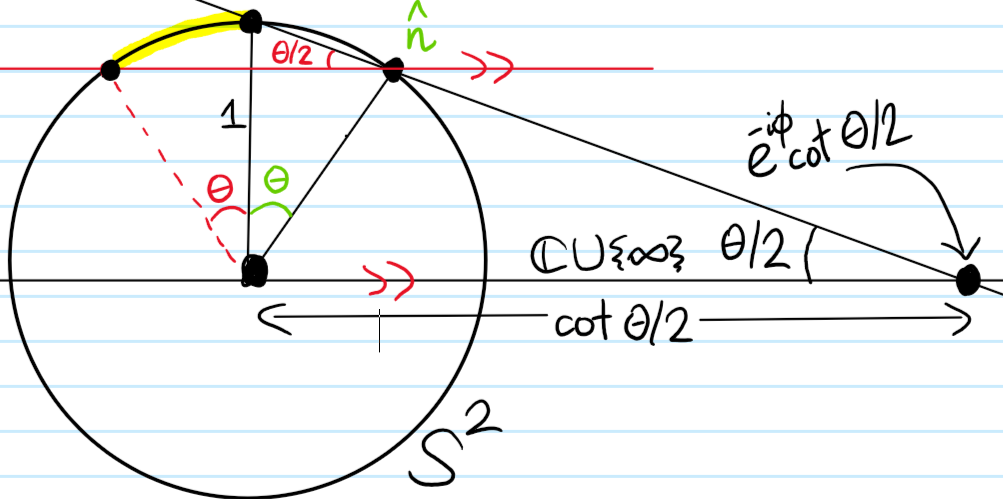
As an aside, there is another nice way to visualize the Bloch mapping \(|m_s=1/2\rangle\mapsto\hat{\textbf n}\), which is a map from \(\textbf C^2\to S^2\). The idea is to decompose it as the composition of a Hopf fibration \(\textbf C^2\to\textbf C\cup\{\infty\}\) onto the extended complex plane \(\textbf C\cup\{\infty\}\), followed by an (inverse) stereographic projection onto an equatorial Riemann sphere \(\textbf C\cup\{\infty\}\to S^2\). Specifically, the Hopf fibration exploits the projective nature of \(P(\textbf C^2)\) by computing the ratio of probability amplitudes \(|\psi\rangle\mapsto\frac{\langle 0|\psi\rangle}{\langle 1|\psi\rangle}\) so in particular \(\cos(\theta/2)|0\rangle+e^{i\phi}\sin(\theta/2)|1\rangle\mapsto e^{-i\phi}\cot(\theta/2)\), and the rest is summarized in this picture:
This discussion has been implicitly focused on the pure quantum states of the qubit, although one could also allow more general mixed ensembles of pure states described by a density operator \(\rho\). In that case, it turns out points inside the Bloch sphere (called the Bloch ball \(|\hat{\textbf n}|<1\)) correspond precisely to such mixed ensembles.
where one can clearly see by setting \(\theta=\pi/2\) in the formula and \(\phi=0,\pi/2,\pi,3\pi/2\) that those cardinal points on the Bloch sphere correspond to the physical qubit states \(|+\rangle=\frac{1}{\sqrt 2}|0\rangle+\frac{1}{\sqrt 2}|1\rangle\), \(|-\rangle=\frac{1}{\sqrt 2}|0\rangle-\frac{1}{\sqrt 2}|1\rangle)\), \(|⟲\rangle=\frac{1}{\sqrt 2}|0\rangle+\frac{i}{\sqrt 2}|1\rangle\), and \(|⟳\rangle=\frac{1}{\sqrt 2}|0\rangle-\frac{i}{\sqrt 2}|1\rangle\) (here, the swirly-arrow notation ⟲,⟳ is actually more of a nod to thinking of the qubit states as photon \(\gamma\) polarization states, specifically as circularly polarized light).
“Qubit Strings” and Quantum Logic Gates
Given a classical bit string \(\xi=b_1b_2b_3…b_N\in\{0,1\}^N\) of length \(|\xi|=N\), the “qubit string” analog of it is given by the obvious isomorphism \(\{0,1\}^N\to\mathcal H_N\) into the state space \(\mathcal H_N\) of an \(N\)-qubit system defined by \(b_1b_2b_3…b_N\mapsto|b_1\rangle\otimes|b_2\rangle\otimes|b_3\rangle\otimes…\otimes|b_N\rangle\). Since there are of course \(2^N\) bit strings \(\xi\in\{0,1\}^N\) of length \(N\), this is indeed an isomorphism with its image defining the canonical unentangled basis \(\text{span}_{\textbf C}\left\{\otimes_{i=1}^N|b_i\rangle:b_i=0\text{ or }1\text{ for all }1\leq i\leq N\right\}=\mathcal H_N\) for \(\mathcal H_N\). In practice, it will often be convenient for “side quantum computations” to “pad” several additional qubits whose states are all initialized “spin-up” \(|0\rangle\) on the Bloch sphere, thus \(|b_1\rangle\otimes|b_2\rangle\otimes|b_3\rangle\otimes…\otimes|b_N\rangle\mapsto |b_1\rangle\otimes|b_2\rangle\otimes|b_3\rangle\otimes…\otimes|b_N\rangle\otimes|0\rangle\otimes|0\rangle\otimes…\otimes|0\rangle\).
Recall that in the circuit model \(\mathcal M_{\text{circuit}}\) of classical computation, the computational steps \(\Gamma_i:\{0,1\}^*\to\{0,1\}^*\) that might comprise a classical algorithm for computing some function \(f:\{0,1\}^*\to\{0,1\}^*\) were a universal set of logic gates like \(\text{AND},\text{OR},\text{NOT}\), etc. Earlier, we just saw that quantumly, we should replace \(N\)-bit strings by their analogous \(N\)-qubit states. What becomes the analog of the logic gates that form the backbone of classical computation in the circuit model? Well, now we just promote them to quantum logic gates acting on multi-qubit states in what should now be thought of as the circuit model of quantum computation. More precisely, an \(N\)-qubitquantum logic gate is any unitaryoperator in \(U\left(\textbf C^{2^N}\right)\) acting on \(N\)-qubit states.
For \(N=1\) qubit, continuing with the earlier example of a qubit realized via the spin angular momentum degree of freedom \(\textbf S\) of an electron \(e^-\), any unitary operator in \(U(\textbf C^2)\) must look like an intrinsic rotation \(e^{-i\Delta{\boldsymbol{\phi}}\cdot\textbf S/\hbar}\in U(\textbf C^2)\) of the electron \(e^-\) (which includes its “spin” axis \(\hat{\textbf n}\)) by an angular displacement \(\Delta{\boldsymbol{\phi}}\in\textbf R^3\). More precisely, for spin \(s=1/2\) quantum particles, we have \([\textbf S]_{|0\rangle,|1\rangle}^{|0\rangle,|1\rangle}=\frac{\hbar}{2}\boldsymbol{\sigma}\), so in the \(S_3\)-eigenbasis \(|0\rangle,|1\rangle\) we have the \(SU(2)\)-analog of Euler’s formula:
where \(\Delta{\boldsymbol{\phi}}=\Delta{\phi}\Delta\hat{\boldsymbol{\phi}}\). In particular, we have the following standard single-qubit quantum logic gates:
where as a special case of Euler’s \(SU(2)\)-formula we have for \(j=0,1,2,3\) that \(\sigma_j=ie^{-i\pi\sigma_j/2}\). However, the \(i\) in front is merely a global \(U(1)\) phase factor which is explicitly ignored in the Bloch \(S^2\) representation of physical qubit states. This is why it is accurate to think of both the Pauli and Hadamard quantum logic gates as encoding \(180^{\circ}=\pi\text{ rad}\) rotations of the qubit state on the Bloch sphere about different axes. Note of course that the Pauli gates are exactly identical to the usual \(\frak{su}\)\((2)\) Pauli matrices. In particular, the Pauli \(X\)-gate is the quantum analog of the classical \(\text{NOT}\) logic gate since when acting on the \(S_3\)-eigenbasis it swaps \(|0\rangle\leftrightarrow|1\rangle\) (of course \(X\) also acts on arbitrary \(\textbf C^2\) superpositions of \(|0\rangle\) and \(|1\rangle\) too on the Bloch \(S^2\) which is the novelty of quantum computing!). And the phase shift gate \(P_{\Delta\phi}\) is really a one-parameter subgroup of quantum logic gates parameterized by the azimuth \(\Delta\phi\in\textbf R\), for instance \(P_{\Delta\phi=\pi}=Z\) and one sometimes also sees the quantum logic gates \(S=P_{\Delta\phi=\pi/2}\) and \(T=P_{\Delta\phi=\pi/4}\). Note that a lot of this notation does clash with standard quantum mechanics notation on \(\textbf R^3\) where \(X,Y,Z\) are often used to denote the Cartesian components of the position observable \(\textbf X\) (although this is partially amended by the existence of the alternative notation \(X_1,X_2,X_3\)). However, an irreparable notational conflict lies in the Hadamard gate \(H=(X+Z)/\sqrt{2}\) where \(H\) is conventionally reserved for the Hamiltonian of a quantum system. For each of these quantum logic gates, there exists a corresponding circuit schematic symbol which (usually) consists simply of enclosing the letter of the gate into a rectangular box and adding an appropriate number of input and output qubit feeds, for example the Hadamard gate:
Just as the classical \(\text{AND}\) and \(\text{OR}\) logic gates accept input bit strings \(\xi\in\{0,1\}^2\) of length \(|\xi|=2\), so there are also two-qubit quantum logic gates in \(U(\textbf C^2\otimes\textbf C^2)\). Here we list a few standard ones:
CX Gate: just as the Pauli \(X\)-gate can be thought of as a quantum NOT gate, the CX gate (called the controlled NOT gate) is a controlled version of the Pauli \(X\)-gate. More precisely, when acting on the unentangled \(2\)-qubit basis \(|0\rangle\otimes|0\rangle, |0\rangle\otimes|1\rangle, |1\rangle\otimes|0\rangle, |1\rangle\otimes|1\rangle\) (also called “the” computational basis for \(2\)-qubit systems), the input state \(|b_1\rangle\) of a controlqubit is acted upon by the identity \(1\) (i.e. nothing happens to it) whereas the input state \(|b_2\rangle\) of a second targetqubit may or may not be acted upon by the Pauli \(X\)-gate \(|b_2\rangle\mapsto X|b_2\rangle\) depending on the control qubit’s input state \(|b_1\rangle\). Such a “truth table” can be expressed as \(CX|b_1\rangle\otimes|b_2\rangle:=|b_1\rangle\otimes X^{b_1}|b_2\rangle=|b_1\rangle\otimes|b_1\text{ XOR } b_2\rangle\) for \(b_1,b_2\in\{0,1\}\), thus showing that the controlled NOT gate \(CX\) can also be viewed as a sort of quantum analog of the classical exclusive or (XOR) logic gate. Note that the action of the controlled NOT gate \(CX\) on arbitrary states in \(\textbf C^{2}\otimes\textbf C^2\) follows from the above truth table by linearity. The controlled NOT gate \(CX\) thus also has matrix representation:
Viewed as a rotation on some kind of entangled Bloch sphere, one also has \(CX=e^{\pm i\frac{\pi}{4}(1-Z_1)\otimes(1-X_2)}\); this can be checked by a direct computation but I still don’t feel I have a strong intuition for why this is right, in particular why it should involve the Pauli \(Z\)-gate of the control qubit?
CY Gate: The controlled Pauli \(Y\)-gate is conceptually identical to the definition of the controlled NOT gate (also called the controlled Pauli \(X\)-gate) just with \(X\mapsto Y\) everywhere in the discussion. The upshot is that \(CY|b_1\rangle\otimes|b_2\rangle=|b_1\rangle\otimes Y^{b_1}|b_2\rangle\) or equivalently:
The controlled Pauli \(Y\)-gate also has a Bloch sphere representation.
CZ Gate: The controlled Pauli \(Z\)-gate is again the same idea (i.e. the idea of having a control qubit to control whether or not a target qubit is acted on by the Pauli \(Z\)-gate), i.e. \(CZ|b_1\rangle\otimes|b_2\rangle=|b_1\rangle\otimes Z^{b_1}|b_2\rangle\) or:
The controlled Pauli \(Z\)-gate also has a Bloch sphere representation.
Measurement
Recall that in quantum mechanics, given an observable \(\textbf X\) (e.g. position) with spectrum \(\textbf x_1,\textbf x_2,…\) and a quantum system in some arbitrary state \(|\psi\rangle\), the Born rule asserts that each \(\textbf x_j\) has probability \(|\langle\textbf x_j|\psi\rangle|^2\) of being the outcome of an \(\textbf X\)-measurement. Specific to the Copenhagen interpretationof quantum measurement is that the state \(|\psi\rangle\) also collapses \(|\psi\rangle\mapsto|\textbf x_j\rangle\) to the \(\textbf X\)-eigenstate \(|\textbf x_j\rangle\) associated to the measured value \(\textbf x_j\). In other words, the measurement of the state \(|\psi\rangle\) randomly projects \(|\psi\rangle\) onto one of the eigenstates of \(\textbf X=\textbf x_1|\textbf x_1\rangle\langle\textbf x_1|+\textbf x_2|\textbf x_2\rangle\langle \textbf x_2|+…\) (this is \(|\psi\rangle\mapsto|\textbf x_j\rangle\langle\textbf x_j|\psi\rangle\cong|\textbf x_j\rangle\)) . However, regardless of the outcome, this measurement process is non-unitary \(\notin U(\mathcal H)\) because a projection \(P^2=P\Rightarrow\det P=0\), being irreversible/non-invertible, must be non-unitary (with the \(\det P=1\) exception that if a quantum system already happens to be in some \(\textbf X\)-eigenstate \(|\textbf x_j\rangle\), then in that case an \(\textbf X\)-measurement simply collapses the state via the identity \(|\textbf x_j\rangle\mapsto|\textbf x_j\rangle\) which is trivially unitary). Another way to convince yourself why measurement is non-unitary is that the inner products \(\langle\psi_1|\psi_2\rangle\mapsto\langle \textbf x_1|\textbf x_2\rangle=\delta_{\textbf x_1,\textbf x_2}\) are not necessarily \(1\) after the measurement (the particular pair of states only has probability \(\text{Tr}()=\sum_{\textbf x\in\Lambda_{\textbf X}}|\langle\textbf x|\psi_1\rangle|^2|\langle\textbf x|\psi_2\rangle|^2\) of being unitary in this sense, assuming they’re unentangled).
Despite being non-unitary, whereas we defined quantum logic gates to be unitary, nothing says we can’t still exploit measurements to our advantage in quantum computation so that in a way they sort of are like just another kind of quantum logic gate (albeit non-unitary and non-deterministic). More precisely, since the measurement will essentially give some concrete bit string, it is common to perform classical computations with the results of measurements; however, note that this doesn’t actually add any novel computational power to quantum computing.
In analogy to the notion of a universal set of logic gates in the circuit model of classical computation, one has the notion of an approximately universal set of quantum logic gates; we want to only consider some finite collection of quantum logic gates as somehow “generating” via compositions all possible quantum logic gates in \(\bigcup_{N\in\textbf N}U\left(\textbf C^{2^N}\right)\), but the group \(\bigcup_{N\in\textbf N}U\left(\textbf C^{2^N}\right)\) has uncountably infinite order whereas any finite collection of quantum logic gates in \(\bigcup_{N\in\textbf N}U\left(\textbf C^{2^N}\right)\) clearly can only generate a countably infinite subgroup (this is similar to how the cyclic subgroup \(C_{\infty}=\{R^n:n\in\textbf N\}\) of \(SO(2)\) generated by some rotation matrix \(R\in SO(2)\) does not actually generate \(SO(2)\) itself, i.e. \(C_{\infty}\neq SO(2)\) again on order grounds \(|C_{\infty}|=\aleph_0<|SO(2)|\) though \(C_{\infty}\) will be dense in \(SO(2)\) provided the generator \(R=\begin{pmatrix}\cos\theta&-\sin\theta\\\sin\theta&\cos\theta\end{pmatrix}\) rotates \(\textbf R^2\) through an irrational angle \(\theta\in\textbf R-\textbf Q\)).
Definition (Approximate Universality): A collection of quantum logic gates \(\mathcal G\subseteq\bigcup_{N\in\textbf N}U\left(\textbf C^{2^N}\right)\) is said to be approximately universal iff for arbitrarily small \(\varepsilon>0\) and any quantum logic gate \(\Gamma\in\bigcup_{N\in\textbf N}U\left(\textbf C^{2^N}\right)\), there exists some quantum logic circuit \(\Gamma_1\circ\Gamma_2\circ…\) with each \(\Gamma_i\in\mathcal G\) such that \(|\Gamma-\Gamma_1\circ\Gamma_2\circ…|<\varepsilon\) in the operator norm, or equivalently \(\sup_{\langle\psi|\psi\rangle=1}|\Gamma|\psi\rangle-\Gamma_1\circ\Gamma_2\circ…|\psi\rangle|<\varepsilon\).
For instance, it can be checked that the collections \(\{\text{CX}\}\cup U(\textbf C^2)\) and \(\{CX,H,T\}\) are approximately universal sets of quantum logic gates. In fact, the former, being uncountably infinite, is actually an exactly universal set of quantum logic gates which means what it sounds like (i.e. \(\varepsilon=0\)).
Mechanical Model of Measurement
I wonder if one can build a mechanical model to illustrate this, e.g. a flashlight mounted on a spinner for an \(\textbf S\)-measurement of a qubit.
Quantum Complexity Classes
Recall that \(\textbf{BPP}\), called the bounded error probabilistic polynomial time complexity class, is the classical complexity class of all decision problems (or equivalently their binary languages \(\mathcal L\subseteq\{0,1\}^*\)) for which there exists a randomized polynomial-time algorithm with “better-than-random” probability of correctly computing the indicator function \(\in_{\mathcal L}:\{0,1\}^*\to\{0,1\}\) on each input bit string \(\xi\in\{0,1\}^*\). The quantum complexity class analog of the classical \(\textbf{BPP}\) complexity class is called \(\textbf{BQP}\), standing for bounded error quantum polynomial time, representing the set of all decision problems for which there exists a polynomial-time quantum circuit/algorithm using some particular approximately universal collection of quantum logic gates that correctly computes the answer to the decision problem at least \(2/3\) of the time (again, the \(2/3\) is sort of arbitrary).
One can check that \(\textbf{BQP}\) is independent of which particular collection of approximately universal quantum logic gates one uses. Just as classically, we have the quantum analog of Cobham’s thesis that \(\textbf{BQP}\) is the class of all “feasible quantum decision problems”. Indeed, there is a simple connection known between \(\textbf{BPP}\) and \(\textbf{BQP}\), namely that \(\textbf{BPP}\subseteq\textbf{BQP}\). The question of whether or not quantum computing is strictly more powerful than classical computing can be phrased roughly as the question: “is \(\textbf{BPP}=\textbf{BQP}\)”? If true, this would mean the answer is “no”.
The purpose of this post is to quickly review some fundamentals of classical computation in order to better appreciate the distinctions between classical computing and quantum computing. Note that the word computation itself, whether classical or quantum, basically just means evaluating functions \(f:\alpha^*\to\alpha^*\) defined on the Kleene closure \(\alpha^*\) of an arbitrary alphabet/set \(\alpha\) (recall that sequences of symbols from the alphabet \(\alpha\) are called stringsover \(\alpha\) with \(\alpha^*=\bigcup_{n\in\textbf N}\alpha^n\) the set of all strings over \(\alpha\)). However, for any at most countable alphabet \(|\alpha|\in\textbf N\cup\{\aleph_0\}\), the Kleene closure \(\alpha^*\) will be countably infinite \(|\alpha^*|=\aleph_0\), so it should therefore be possible to exhibit a injection \(\alpha^*\to\alpha_{\text{binary}}^*\) from strings in \(\alpha^*\) to bit strings in \(\alpha_{\text{binary}}^*\) where \(\alpha_{\text{binary}}:=\{0,1\}\) is the binary alphabet. In turn, this simply means finding a (binary)encoding \(\mathcal E:\alpha\to\alpha_{\text{binary}}^*\) at the level of the individual symbols in the alphabet \(\alpha\) into bit strings in \(\alpha_{\text{binary}}^*\) and then concatenating together bit strings for individual symbols in \(\alpha\) to obtain bit strings for strings in \(\alpha^*\). In image processing for instance, such an encoding \(\mathcal E\) would be thought of as lossless compression of the data/symbols in the alphabet \(\alpha\), and there are many possible encoding schemes depending on the situation, for instance a fixed-length encoding \(\mathcal E_{\text{FL}}\), or variable-length encodings such as run-length encoding \(\mathcal E_{\text{RL}}\) or Huffman encoding \(\mathcal E_{\text{Huffman}}\). If one uses a fixed-length encoding \(\mathcal E_{\text{FL}}\), then the overheadcost associated with \(\mathcal E_{\text{FL}}\) is linear \(\mathcal E_{\text{FL}}(a_1+a_2)=\mathcal E_{\text{FL}}(a_1)+\mathcal E_{\text{FL}}(a_2)\) for all symbols \(a_1,a_2\in\alpha\) (where here we adapt the Pythonic meaning of \(+\) as a string concatenation; note that the encoding \(\mathcal E_{\text{FL}}\) is technically only defined on the alphabet \(\alpha\), so the statement above is more of a definition of how to extend the domain of \(\mathcal E_{\text{FL}}\) from \(\alpha\) to \(\alpha^*\)). This discussion is just to say that henceforth we can assume without loss of generality that the alphabet \(\alpha=\alpha_{\text{binary}}\) is just the binary alphabet, and so all computations will be concerned with evaluating functions \(f:\{0,1\}^*\to\{0,1\}^*\) which map input bit strings to output bit strings.
Defining a binary language \(\mathcal L\) to be any collection of bit strings \(\mathcal L\subseteq\{0,1\}^*\), the decision problem for \(\mathcal L\) is to compute the indicator function \(\in_{\mathcal L}:\{0,1\}^*\to\{0,1\}^*\) of \(\mathcal L\) defined for all input bit strings \(\xi\in\{0,1\}^*\) by the Iverson bracket \(\in_{\mathcal L}(\xi):=[\xi\in\mathcal L]\). Note however that although in general we allow the codomain \(\{0,1\}^*\) of the function \(\in_{\mathcal L}\) being computed to consist of output bit strings of arbitrary length, in fact for binary language decision problems the range \(\in_{\mathcal L}(\{0,1\}^*)\) as manifest in the Iverson bracket is restricted to the \(2\) possible one-bit strings \(\in_{\mathcal L}(\{0,1\}^*)=\{0,1\}\subseteq\{0,1\}^*\). A very important example of a decision problem is primality testing where the binary language \(\mathcal L:=\{10,11,101,111,1011,…\}\) consists of all the prime numbers. The decision problem of primality testing is a decidable decision problem by virtue of e.g. the AKS primality test. On the contrary, there unfortunately do also exist undecidable decision problems, examples being the halting problem, Hilbert’s tenth problem, etc. The notion of decidability is specific to decision problems and generalizes to non-decision problems via the notion of computability.
Circuit Model of Classical Computation
Recall that a computation is an evaluation of a function \(f:\{0,1\}^*\to\{0,1\}^*\). A computational model \(\mathcal M\) is any collection \(\mathcal M=\{\Gamma_i:\{0,1\}^*\to\{0,1\}^*|\Gamma_i(\xi)\in O_{|\xi|\to\infty}(1)\}\) of computational steps \(\Gamma_i\in\mathcal M\) considered legal within the framework of \(\mathcal M\), and any well-defined sequence \(\Gamma_1\circ\Gamma_2\circ\Gamma_3…=f\) of such computational steps that compose to the function \(f\) of interest is called an algorithmfor computing \(f\) in \(\mathcal M\). Historically, many computational models \(\mathcal M\) (e.g. Turing machines, general recursive functions, lambda calculus, Post machines, register machines) have been proposed in which the nature of the allowed computational steps \(\Gamma_i\in\mathcal M\) seem a priori to give rise to different classes of computable functions \(f\) (i.e. functions \(f\) for which there even exists \(\exists\) some algorithm \(\Gamma_1\circ\Gamma_2\circ\Gamma_3…=f\) for computing \(f\)). However, the Church-Turing thesis is an informal conjecture/axiom in computability theory which roughly asserts that any “reasonable” computational model \(\mathcal M\) one can dream up will in fact have neither greater nor less computing power compared with any other “reasonable” computational model \(\mathcal M’\cong\mathcal M\). Thus, for the purposes of a smoother transition from classical computing to quantum computing, we will henceforth take the circuit model \(\mathcal M_{\text{circuit}}\) to be our computational model. In the circuit model of classical computation \(\mathcal M_{\text{circuit}}\), the allowed computational steps are the \(3\) logic gates \(\mathcal M_{\text{circuit}}=\{\text{AND},\text{OR},\text{NOT}\}\) which form a universal set for arbitrary logic circuits/Boolean functions (though the \(\text{OR}\) gate is actually redundant! see here). For instance, binary adder/multiplier logic circuits are not considered to be computational steps in the circuit model \(\mathcal M_{\text{circuit}}\) because say for two input bit strings \(\xi_1,\xi_2\) of the same length \(n=|\xi_1|=|\xi_2|\) they are not \(O_{n\to\infty}(1)\) as required.
Randomized Classical Computational Models
In anticipation of the randomness inherent in outputs of quantum computations, it will be helpful to quickly review what it means for a classical computational model (such as the circuit model of classical computation) to be randomized. This means that when computing a function \(f:\{0,1\}^*\to\{0,1\}^*\), any input bit string \(\xi\in\{0,1\}^*\) is also concatenated \(\xi\mapsto \xi+\xi_{\text{random}}\) with a uniformly random input bit string from a hypothetical random number generator such as \(\xi_{\text{random}}=011011010001001\in\{0,1\}^*\) (so for each run of the computation, even for the same input bit string \(\xi\), the input bit string \(\xi_{\text{random}}\) will probably be different from the previous run and thus the output bit string of the computation will be a sample from a probability distribution) but otherwise one now just chugs the total input bit string \(\xi+\xi_{\text{random}}\) through some sequence of computational steps \(\Gamma_1,\Gamma_2,…\) within that computational model. For instance, in the circuit model, if one desires a particular logic gate \(\Gamma\) in a computation to act with \(50\%\) probability as an \(\text{AND}\) gate and with \(50\%\) probability as an \(\text{OR}\) gate, then one can define \(\Gamma:\{0,1\}^3\to\{0,1\}\) to take an input bit string \(b_1b_2b_3\) of length \(3\) (i.e. \(3\) input bits) but where say the third input bit \(b_3\) is one of the random input bits in the string \(\xi_{\text{random}}\) and determines the nature of the logic gate \(\Gamma\) according to:
Among randomized computational models, there are \(2\) subclasses: Las Vegas algorithms such as the quicksort algorithm which emphasize correctness of the computational output bit string and Monte Carlo “algorithms” such as Miller-Rabin primality testing which emphasize high probability of correctness of the computational output bit string.
Finally, a note about determinism in computational models. Classical computational models are always deterministic because \(f\) is a function. I would argue that even randomized classical computational models are deterministic because, if for two runs the exact same random bit string \(\xi_{\text{random}}\) happens to be inputted, then the output bit string \(f(\xi+\xi_{\text{random}})\in\{0,1\}^*\) must deterministically be the same. So what would be a non-deterministic computational model? Basically, the God-like magical power of being able to just instantaneously “guess” the correct output bit string \(f(\xi)\in\{0,1\}^*\) for any input bit string \(\xi\in\{0,1\}^*\). Such a non-deterministic computer cannot exist, but is an important theoretical construct for defining the nondeterministic polynomial timecomplexity class \(NP\) which will be elaborated in the following section.
ClassicalComplexity Classes
If, in some computational model \(\mathcal M\), someone has found an algorithm \(\Gamma_1\circ\Gamma_2\circ\Gamma_3…=f\) for computing \(f\) (hopefully correctly or at least with high probability of being correct such as in Monte Carlo “algorithms”), then one can always ask about how efficient the algorithm \(\Gamma_1\circ\Gamma_2\circ\Gamma_3…\) is at computing \(f\). This is, in computer science lingo, a question of the algorithm’s complexity. Associated to any algorithm \(\Gamma_1\circ\Gamma_2\circ\Gamma_3…\) are \(2\) distinct kinds of complexity: time complexity (i.e. the number of computational steps \(\Gamma_i\) in the algorithm sequence \(\Gamma_1\circ\Gamma_2\circ\Gamma_3…\)) and space complexity (i.e. “amount” of memory/”RAM” used during execution of the algorithm sequence \(\Gamma_1\circ\Gamma_2\circ\Gamma_3…\)). In general, both the time complexity and space complexity of an algorithm \(\Gamma_1\circ\Gamma_2\circ\Gamma_3…\) are to be viewed as functions of which particular input bit string \(\xi\in\{0,1\}^*\) is fed into the algorithm \(\xi\mapsto\Gamma_1\circ\Gamma_2\circ\Gamma_3…(\xi)\) where in general, input bit strings \(\xi\in\{0,1\}^*\) of longer length \(|\xi|\) may be expected to require greater time complexity \(T(\xi)\) and space complexity \(Sp(\xi)\). More precisely, one is often interested in the behavior of the worst-casetime complexity \(T^*(n):=\sup_{\xi\in\{0,1\}^n}T(\xi)\) of the algorithm \(\Gamma_1\circ\Gamma_2\circ\Gamma_3…\) in the asymptotic \(n\to\infty\) limit of longer and longer input bit strings \(\xi\in\{0,1\}^*\) and likewise the behavior of the worst-case space complexity \(Sp^*(n):=\sup_{\xi\in\{0,1\}^n}Sp(\xi)\) in the asymptotic \(n\to\infty\) limit. Sometimes though it’s also interesting to analyze the algorithm’s average time complexity \(\bar T(n):=\frac{1}{2^n}\sum_{\xi\in\{0,1\}^n}T(\xi)\) or the averagespace complexity \(\bar{Sp}(n):=\frac{1}{2^n}\sum_{\xi\in\{0,1\}^n}Sp(\xi)\), both asymptotically \(n\to\infty\).
Example: For a list of length \(n\in\textbf N\), the linear search algorithm has (both worst-case and average) time complexity that scales asymptotically as \(T^*_{\text{linear search}}(n),\bar T_{\text{linear search}}(n)\in O_{n\to\infty}(n)\) but (both worst-case and average) space complexity that scales asymptotically as \(Sp^*_{\text{linear search}}(n),\bar{Sp}_{\text{linear search}}(n)\in O_{n\to\infty}(1)\). By contrast, the merge sort algorithm has (both worst-case and average) time complexity that scales asymptotically as \(T^*_{\text{merge sort}}(n),\bar T_{\text{merge sort}}(n)\in O_{n\to\infty}(n\log n)\) and (both worst-case and average) space complexity that scales asymptotically as \(Sp^*_{\text{merge sort}}(n),\bar{Sp}_{\text{merge sort}}(n)\in O_{n\to\infty}(n)\). This is obvious, but note that searching a list vs. sorting a list are different computations so one cannot just directly compare these algorithm’s asymptotic spacetime complexities to declare linear search is “more efficient” than merge sort; however binary search is indeed an asymptotically more efficient search algorithm than linear search as measured by their spacetime complexities in the worst-case or averaged senses.
Recall that a decision problem concerns the computation of the indicator function \(\in_{\mathcal L}:\{0,1\}^*\to\{0,1\}\) of a binary language \(\mathcal L\subseteq\{0,1\}^*\) of bit strings. To this effect, we define:
Definition (\(\textbf P\)): The polynomial time complexity class \(\textbf P\) is defined to be the set of all binary languages \(\mathcal L\), or equivalently decision problems, for which there exists an algorithm \(\Gamma_1\circ\Gamma_2\circ\Gamma_3…=\in_{\mathcal L}\) that computes the indicator function \(\in_{\mathcal L}:\{0,1\}^*\to\{0,1\}\) with worst-case time complexity \(T^*_{\Gamma_1\circ\Gamma_2\circ\Gamma_3…}(n)\in\bigcup_{p\in\textbf N}O_{n\to\infty}(n^p)\).
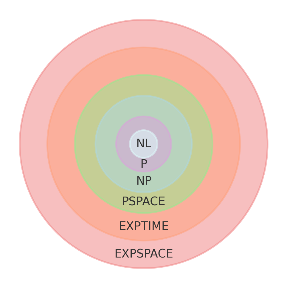
Notice in the definition that we haven’t specified a computational model \(\mathcal M\) from which we derive the computational steps \(\Gamma_i\in\mathcal M\). Indeed, it turns out that the polynomial time complexity class \(\textbf P\) (as with all other complexity classes) is robust with respect to whichever computational model \(\mathcal M\) one chooses to use in the sense that a given binary language/decision problem is in \(\textbf P\) in one computational model \(\mathcal M\) if and only if it’s in \(\textbf P\) in any other Church-Turing equivalent computational model \(\mathcal M’\). Also, note that the polynomial time complexity class \(\textbf P\) doesn’t a priori impose any constraints on the (worst-case or average) space complexity \(Sp_{\Gamma_1\circ\Gamma_2\circ\Gamma_3…}(n)\) of the algorithm. Nonetheless, one can show that \(\textbf P\subseteq \textbf{PSPACE}\) where \(\textbf{PSPACE}\) is the polynomial space complexity class defined verbatim to the polynomial time complexity class \(\textbf P\) except replacing the word “time” with “space” and thus \(T\mapsto Sp\). Whether or not the reverse inclusion \(\textbf{PSPACE}\subseteq \textbf{P}\) is true is still an open question!
Examples: Primality testing is a decision problem which recently (thanks to the AKS primality test) has been shown to be in the polynomial time complexity class \(\textbf P\) (and therefore also in \(\textbf{PSPACE}\)). Note that a naive primality test in which we take a given \(N\in\textbf Z^+\) and divide it by each positive integer \(\leq\sqrt{N}\) does not constitute a polynomial-time algorithm for primality testing. This is because \(\sqrt{N}=2^{\log_2(N)/2}\), but \(n:=\log_2(N)\) is the actual length of the input bit string for \(N\) so therefore we see that this naive primality test algorithm \(T^*_{\text{naive primality test}}(n)\in O_{n\to\infty}(2^n)\) is actually exponential-time. Although it may seem that list searching/ sorting problems are also members of the polynomial time complexity class \(\textbf P\) (thanks to e.g. linear search, binary search, merge sort, etc.), this is strictly speaking only the case if one reframes the original search/sorting problem into a decision problem like “does this list contain the bit string \(1011\)” so that the binary language \(\mathcal L=\{1011\}\) is singleton. Otherwise, one would more accurately consider list searching/sorting problems to be in the complexity class \(\textbf{FP}\) of “functions”.
Owing to the existence of randomized computation leading to randomized algorithms (in particular Monte Carlo algorithms), we also have:
Definition (\(\textbf{BPP}\)): The bounded error probabilistic polynomial time complexity class \(\textbf{BPP}\) is defined to be the set of all binary languages \(\mathcal L\), or equivalently decision problems, for which there exists a randomized algorithm \(\Gamma_1\circ\Gamma_2\circ\Gamma_3…\approx \in_{\mathcal L}\) that attempts to compute the indicator function \(\in_{\mathcal L}:\{0,1\}^*\to\{0,1\}\) with worst-case time complexity \(T^*_{\Gamma_1\circ\Gamma_2\circ\Gamma_3…}(n)\in\bigcup_{q\in\textbf N}O_{n\to\infty}(n^q)\) and correctness probability \(p(\xi)\in(1/2,1]\) for all input bit strings \(\xi\in\{0,1\}^*\) (commonly just declared to be \(\geq 2/3\), though this is arbitrary because one can consider a new algorithm defined by running arbitrarily many Bernoulli trials of the original algorithm, taking the majority decision, and applying the Chernoff bound; thus it suffices to find a Monte Carlo algorithm with \(p(\xi)\in(1/2,1)\) or a Las Vegas algorithm with \(p(\xi)=1\)).
According toCobham’s thesis, the bounded error probabilistic polynomial time complexity class \(\textbf{BPP}\) (with \(\textbf P\subseteq\textbf{BPP}\) obviously contained therein) of decision problems are considered “classically feasible decision problems” and so the goal of computer scientists is to prove that various \(\mathcal L\)-decision problems are in \(\textbf{BPP}\) by devising clever (possibly randomized) polynomial-time algorithms to compute their corresponding indicator functions (either always correctly or more often than not correctly!). Decision problems which are not in \(\textbf{BPP}\) (or more precisely, haven’t been shown to be in \(\textbf{BPP}\) because no one has discovered a polynomial-time algorithm to compute their indicator functions yet) are therefore the hardest decision problems to solve. Among these are:
Definition (\(\textbf{NP}\)): The nondeterministic polynomial time complexity class \(\textbf{NP}\) is defined to be the set of all binary languages \(\mathcal L\), or equivalently decision problems, for which there exists a nondeterministic algorithm \(\Gamma_{\text{God}}=\in_{\mathcal L}\) that computes the indicator function \(\in_{\mathcal L}:\{0,1\}^*\to\{0,1\}\) with worst-case time complexity \(T^*_{\Gamma_{\text{God}}}(n)\in\bigcup_{p\in\textbf N}O_{n\to\infty}(n^p)\).
In other words, an \(\mathcal L\)-decision problem is in \(\mathcal L\in\textbf{NP}\) iff its corresponding \(\mathcal L\)-verification decision problem concerning the computation of the function \([\xi\in]\) is in \(\textbf P\). The following diagram summarizes the current state of knowledge as of \(2024\), October \(3\)rd (note that the relationship between \(\textbf{BPP}\) and \(\textbf{NP}\) is still not known!):
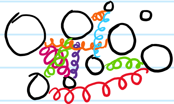
Problem #\(1\): What does the phrase “\(N\) coupled harmonic oscillators” mean?
Solution #\(1\): Basically, just think of \(N\) masses \(m_1,m_2,…,m_N\) with some arbitrarily complicated network of springs (each of which could have different spring constants) connecting various pairs of masses together:
Problem #\(2\): Rephrase Solution #\(1\) in more mathematical terms.
Solution #\(2\): The idea is that there are \(N\) degrees of freedom \(x_1,x_2,…,x_N\) and the second time derivative of each one is given by some linear combination of the \(N\) degrees of freedom; packaging into a vector \(\textbf x:=(x_1,x_2,…,x_N)^T\in\textbf R^N\), this means that there exists an \(N\times N\) matrix \(\omega^2\) (independent of \(t\)) such that:
\[\ddot{\textbf x}=-\omega^2\textbf x\]
Problem #\(3\): In general, how does one solve the second-order ODE in Solution #\(2\)?
Solution #\(3\): One way is to first rewrite it as a first-order ODE:
and using \(\begin{pmatrix}0&1\\-\omega^2&0\end{pmatrix}^2=-\begin{pmatrix}\omega^2&0\\0&\omega^2\end{pmatrix}\), one has the self-consistent solutions:
The point is that one needs an efficient way to evaluate powers \(\omega^{2n}\) of the matrix \(\omega^2\) appearing in the equation of motion \(\ddot{\textbf x}=-\omega^2\textbf x\); the standard way to do this is to diagonalize \(\omega^2\).
Problem #\(5\): Interpret the diagonalization of \(\omega^2\) in Solution #\(4\) as a physicist.
Solution #\(5\): Each eigenspace of \(\omega^2\) is called a normal mode of the corresponding system of coupled harmonic oscillators, i.e. a normal mode should be thought of as a pair \((\omega_0,\ker(\omega^2-\omega_0^21))\); since \(\omega^2\) is an \(N\times N\) matrix, there will in general be \(N\) normal modes (assuming \(\omega^2\) is diagonalizable which in practice will always be the case). Viewed in this way, the general dynamics of \(N\) coupled harmonic oscillators consists of a superposition of the \(N\) normal modes of the system, with the coefficients in this superposition determined by the initial conditions \(\textbf x(0),\dot{\textbf x}(0)\).
Physically, because a normal mode is defined by a single eigenfrequency \(\omega_0\), it means that if one were to release the system with exactly the right initial conditions to excite only that one specific normal mode, then all \(N\) coupled harmonic oscillators would oscillate at the same frequency \(\omega_0\) with some relative amplitudes and relative phases between each of their oscillations as encoded in the corresponding eigenspace \(\ker(\omega^2-\omega_0^21)\).
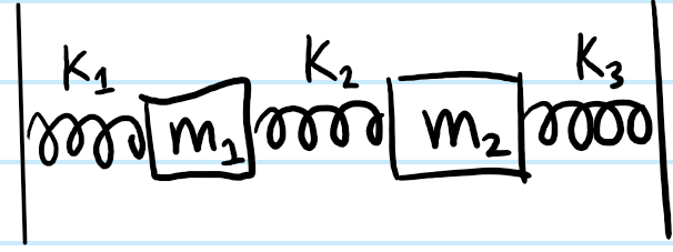
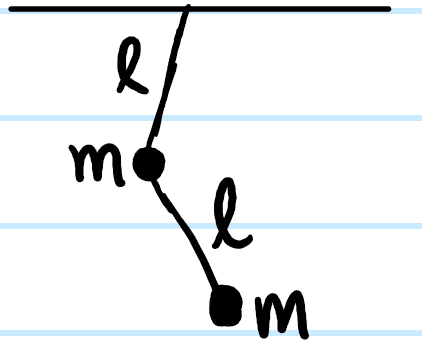
Problem #\(6\): Determine the normal modes of the following systems of coupled harmonic oscillators:
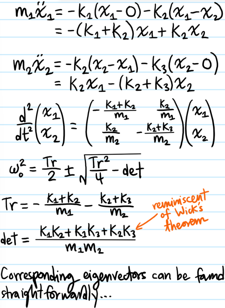
Solution #\(6\): For the \(2\) masses connected to each other and to immoveable walls (equivalent to having infinite masses at those locations):
Needless to say for generic \(m_1,m_2,k_1,k_2,k_3\) the normal modes are not so straightforward either. There are of course also many variations of this setup, for instance \(k_3=0\) (i.e. just no wall there) or having \(m_1=m_2\) and \(k_1=k_2=k_3\), etc.
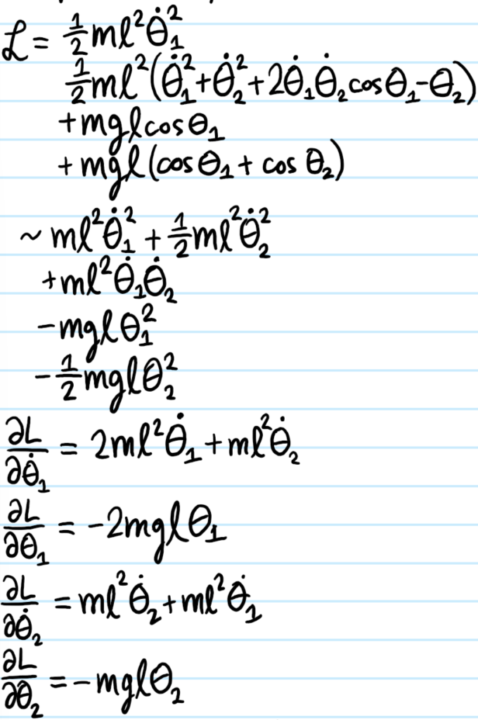
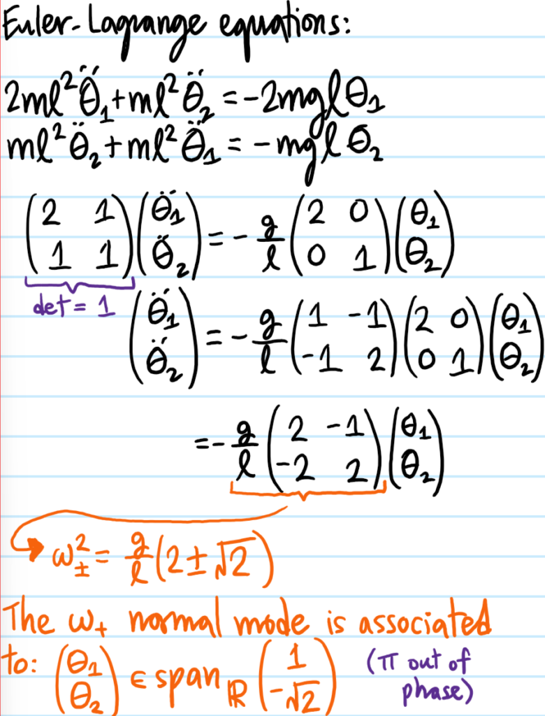
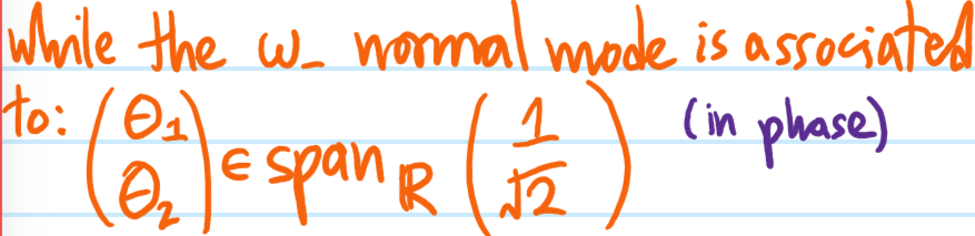
For the double pendulum, it is of course the standard example of a nonlinear dynamical system, but it has a stable fixed point at \(\theta_1=\theta_2=0\) so one can linearize the system about it to obtain \(2\) coupled harmonic oscillators:
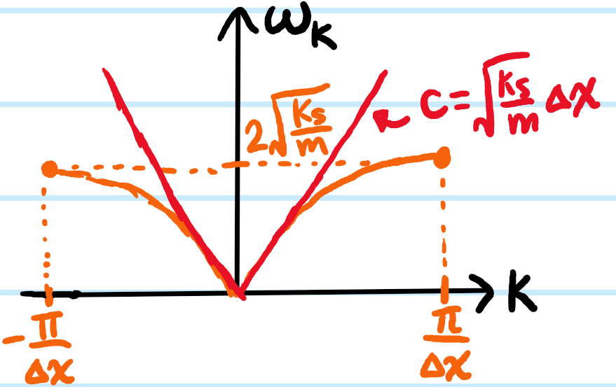
Problem #\(7\): Consider extending the first system from Problem #\(6\) from \(N=2\) to \(N\gg 1\) identical masses \(m\) connected by identical springs \(k_s\); in condensed matter physics this is known as the \(1\)D monatomic chain, a classical toy model of a solid. Write down the equation of motion for the displacement \(x_n(t)\) of the \(n\)th atom about its equilibrium where \(2\leq n\leq N-1\); in order for this equation to also be valid for the boundary atoms \(n=1,N\), what (somewhat artificial) assumption does one need to make about the topology of the chain?
Solution #\(7\): For each \(n=2,3,…,N-2,N-1\), the longitudinal displacement satisfies Newton’s second law in the form:
If one were to use the same setup as in Problem #\(6\) where the boundary masses are simply connected to walls, or perhaps not connected to anything at all, then this equation of motion would not be valid for \(n=1,N\); however if one imposes an \(S^1\) topology on the chain by identifying \(x_n=x_m\pmod N\) (as if the \(N\) masses had been stringed along a circle instead of a line), then the equation becomes valid for \(n=1,N\) as well. It is for this simple convenient reason that periodic boundary conditions are commonly assumed; for \(N\gg 1\) it is intuitively plausible that the exact choice of boundary conditions shouldn’t affect bulk physics as bulk\(\cap\)boundary\(=\emptyset\).
Problem #\(8\): If \(\Delta x\) denotes the lattice spacing between adjacent masses \(m\) when the entire monatomic chain is at rest, show that the equation of motion coarse grains in the limit \(\Delta x\to 0\) to the \(1\)D free, dispersionless wave equation:
where \(c^2=\frac{k_s}{m}(\Delta x)^2\), and the longitudinal displacement \(x_n\mapsto\psi\) has been promoted to a scalar field (and renamed to avoid confusion with the spatial coordinate \(x\)).
Solution #\(8\): One simply has to invoke the symmetric limit formulation of the second derivative:
Problem #\(9\): Motivated by the result of Solution #\(8\), what is a reasonable ansatz for the longitudinal displacement \(x_n(t)\)? What is the connection between this result and the earlier discussion of normal modes?
Solution #\(9\): Motivated by the usual plane wave solutions \(\psi(x,t)=e^{i(kx-\omega_k t)}\) (with linear dispersion relation \(\omega_k=ck\)) that form the usual Fourier basis for arbitrary solutions to the wave equation, one can similarly write \(x_n(t)=e^{i(kn\Delta x-\omega_k t)}\), where \(x\mapsto n\Delta x\) is the analog of the spatial coordinate. Plugging this into the equation of motion, one finds instead that e.g. a sound wavepacket will disperse as it propagates through this monatomic chain:
which can be plotted in the first Brillouin zone \(k\Delta x\in[-\pi,\pi)\):
Furthermore, the low-\(|k|\) limit of the group (or in this case phase) velocity \(c=\frac{\partial\omega}{\partial k}\) agrees with the linear dispersion relation from Problem #\(8\); this makes sense because the wave equation was obtained by coarse graining which is equivalent to assuming \(|k|\Delta x\ll 1\).
In general, whenever one finds a linear dispersion relation \(\omega_k\sim k\), it suggests massless particles (e.g. photons, phonons); this is to be contrasted with quadratic dispersion relations \(\omega_k\sim k^2\) which suggest massive particles (e.g. electrons in a tight-binding lattice).
Finally, to connect back to normal modes, because one has \(N\gg 1\) atoms coupled harmonically in the monatomic chain, one of course expects the system to have \(N\gg 1\) normal modes. And indeed the ansatz \(x_n(t)=e^{i(kn\Delta x-\omega_k t)}\) is exactly the form of a normal mode in which all atoms oscillate at the same frequency \(\omega_k\) and (on symmetry grounds) with the same amplitude, but where there is the same constant phase offset of \(x_{n+1}(t)/x_n(t)=e^{ik\Delta x}\) between each pair of adjacent atoms in the chain (again, this phase shift is the same between all pairs of atoms on symmetry grounds). Hopefully this gives the vibe of a sound wave propagating through the chain.
It’s as if we guessed ahead of time the eigenvectors \(x_n(t)\) of the matrix \(\omega^2\) in Solution #\(2\) and then simply acted with \(\omega^2\) on the ansatz eigenvector \( x_n(t)\) and checked that it scales by an eigenvalue \(\omega_k^2\) which gave the dispersion relation (again, usually one finds eigenvalues of a matrix before eigenvectors! This was only possible because of the symmetry; in general, circulant matrices are always diagonalized by the discrete Fourier transform).
Finally, as a minor aside, the earlier choice of periodic boundary condition \(x_{n}(t)\equiv x_{m}(t)\pmod N\) forces \(e^{ikN\Delta x}=1\) which quantizes the wavenumber \(k_m=\frac{2\pi m}{N\Delta x}\) for \(m\in\textbf Z\) (not to be confused with the mass \(m\) obviously); within the first Brillouin zone, there are \(N\) values of \(m=-N/2,…,N/2\) which are the \(N\) normal modes of the chain (i.e. each \(m\to k_m\to\omega_{k_m}\to\omega^2_{k_m}\) corresponding to one of the \(N\) eigenvalues of the \(N\times N\) \(\omega^2\) matrix).
So technically, for a finite monatomic chain of \(N\) atoms, there are only \(N\) combinations of \((k,\omega_k)\) on the dispersion graph which represent permissible normal modes, but as \(N\to\infty\) this quantization will become invisible with \(k,\omega_k\in\textbf R\).
Problem #\(10\): Repeat Problem #\(9\) but for a diatomic chain of masses. Hence show that there are \(2\) qualitatively different classes of normal modes that can be excited in this system, called acoustic modes and optical modes with respective dispersion relations:
in order to get a non-trivial normal mode \((\alpha,\beta)\neq (0,0)\), require the determinant to vanish which gives the desired result (it is instructive to check that the quantity under the square root is indeed non-negative as required by Hermiticity of the matrix).
It is instructive to look at how the diatomic chain reduces to the monatomic chain by setting \(m=M=2\mu\). Then the optical branch becomes:
Nevertheless, in a monatomic chain there are no optical phonons, only acoustic phonons because it is \(\Delta x\)-periodic so the Brillouin zone ranges from \(-\pi\leq k\Delta x<\pi\) rather than \(-\pi/2\leq k\Delta x<\pi/2\) as appropriate for a \(2\Delta x\)-periodic diatomic chain (remember, there must still be \(N\) normal modes!). Nevertheless, this does provide intuition for why there is an optical branch (and this procedure is also generalizable to triatomic, etc. chains):
i.e. because the Brillouin zone of the diatomic chain is half as wide as the monatomic chain, so in the reduced Brillouin zone scheme for the diatomic chain, the parts from the monatomic chain are reflected inward, giving the \(\sim\cos\) shape of the optical branch (note these branches are very much analogous to a band structure for phonons instead of electrons; indeed because in a generic diatomic chain \(m\neq M\), this is the origin of the “branch gap” \((\omega_+-\omega_-)_{k=\pm\pi/2\Delta x}=\sqrt{2k_s}|m^{-1/2}-M^{-1/2}|\) between the acoustic and optical branches of the phonon spectrum \(\omega_k\) at the boundary of the Brillouin zone, cf. band gaps. In particular, \((\omega_+-\omega_-)_{k=\pm\pi/2\Delta x}\to 0\) as \(m\to M\)).
Back to the diatomic chain, for \(|k|\Delta x\ll 1\):
and flatten to zero \(\partial\omega_{\pm}/\partial k\to 0\) at the boundary \(k\to\pm\pi/2\Delta x\) of the Brillouin zone, just as one finds in band structure (e.g. for nearly free electrons). All this is summarized in this refined picture:
Problem #\(11\): How do the atoms in the diatomic chain actually move in acoustic vs. optical normal modes?
Solution #\(11\): In general, the phasor ratios of \(m\) vs. \(M\) atom displacements (viewed as functions of \(k\)) are:
So at low-\(k\), the diatomic chain in an acoustic normal mode looks like neighbouring atoms oscillating in phase with equal amplitude whereas the optical mode looks like a \(\pi\)-radian out-of-phase oscillation with the lighter atoms oscillating more than the heavier atoms by the mass ratio \(M/m\), as intuitively reasonable. This also explains the name “optical branch”; if the atoms in the diatomic chain are in fact ions of opposite charge as in an \(\text{NaCl}\) crystal, then one has pairs of oscillating electric dipoles which can couple to light.
Meanwhile, at the boundary of the Brillouin zone, one finds:
where although \(\sec\pm\pi/2=\infty\) diverges, causing \((\beta/\alpha)_-=\infty\), actually the factor in front goes to zero even faster than the secant diverges as \(k\to\pm\pi/2\Delta x\) so that actually \((\beta/\alpha)_+=0\). This is a (longitudinal) standing wave! i.e. in the optical mode, one has nodes at the heavier atoms \(M\) while the light atoms represent displacement antinodes, and vice versa in the acoustic mode (intuitively, \(k=\pi/2\Delta x\Leftrightarrow\lambda=4\Delta x\)).
Notice the group velocity \((\partial\omega/\partial k)_{k=\pm\pi/2\Delta x}\) also tends to zero at the Brillouin zone boundary…that’s just another way of saying it’s a standing wave!
Another useful intuition is that, say near \(k=0\), the acoustic and optical normal modes look the way they do such that atoms can be paired up at any moment in time with equal and opposite momenta, giving the overall collective excitation/phonon also zero momentum! So there is a direct connection between \(mv\) momentum and \(\hbar k\) momentum (ACTUALLY ARE WE SURE THIS IS TRUE?).
Problem #\(12\): Just to emphasize again: on the one hand, one can generically refer to \(\omega_k\) as a dispersion relation for a particular kind of wave; here what is a better name for \(\omega_k\)?
Solution #\(12\): The phrase “normal mode spectrum” is useful to keep in mind.
The purpose of this post is to answer some questions posed to me by ChatGPT regarding my understanding of the \(z\)-transform in digital signal processing and mathematics more broadly. My inquiry to it was simply: “Ask me some questions to test my understanding of the \(z\)-transform”. Here were ChatGPT’s questions, followed by my answers.
Question #1: What is the general definition of the \(z\)-transform for a discrete-time signal \(x_n\)?
My Answer: Given a sequence \((x_n)_{n=-\infty}^{\infty}\) of (possibly complex) numbers, the \(z\)-transform \(X(z)\) of the sequence \((x_n)_{n\in\textbf Z}\) is a map \(z\in\textbf C\to X(z)\in\textbf C\) on the complex plane \(\textbf C\) defined by the formal Laurent series about the origin:
\[X(z):=\sum_{n\in\textbf Z}x_n z^{-n}\]
It is also denoted \(X(z)=\mathcal Z\{x\}(z)\). More precisely, this is the bilateral \(z\)-transform and one can also consider sequences \((x_n)_{n=0}^{\infty}\) defined only for non-negative \(n\geq 0\) along with the unilateral \(z\)-transform \(X(z):=\sum_{n=0}^{\infty}x_n z^{-n}\). This then resembles the form of an (ordinary) generating function for the sequence \((x_n)_{n=0}^\infty\).
Question #2: For the discrete unit impulse signal \(x_n=\delta_{n,0}\), what is the z-transform?
My Answer: As an Einstein series over \(n\in\textbf Z\), we have \(X(z)=\delta_{n,0}z^{-n}\) which contracts to \(X(z)=z^{-0}=1\).
Question #3: What does the region of convergence (ROC) in the \(z\)-transform tell you about a system or signal?
My Answer: The region of convergence (ROC), perhaps more descriptively called the annulus of convergence, is simply the set of all \(z\in\textbf C\) for which the formal Laurent series defining the \(z\)-transform is actually a convergent infinite series. It provides information about both stability and causality.
Question #4: How do you determine if a discrete-time dynamical system is stable using the \(z\)-transform?
My Answer: Recalling that a discrete-time dynamical system \((x_n)_{n=-\infty}^{\infty}\) is said to be stable (or asymptotically stable) iff \(\lim_{n\to\infty}x_n=0\), the sufficient and necessary criterion for stability is that the poles of its \(z\)-transform \(X(z)\) must all lie in the interior of \(U(1)\) i.e. \(|z_{\text{poles}}|<1\).
Question #5: Compute the \(z\)-transform of \(x_n=\left(-\frac{1}{2}\right)^nu_n\) where \(u_n\) is the unit step function \(u_n:=[n\geq 0]\).
Question #6: Explain how the \(z\)-transform simplifies the process of convolution between two discrete-time signals \(x_n,y_n\).
My Answer: The \(z\)-transform of the discrete convolution \((x*y)_n\) of two discrete-time signals \(x_n,y_n\) is the product of their individual \(z\)-transforms. This is one version of the convolution theorem:
Put another way, to compute the convolution \((x*y)_n\) of two discrete-time signals, one can instead compute \((x*y)_n=\mathcal Z^{-1}(\mathcal Z\{x\}(z)\mathcal Z\{y\}(z))_n\).
Question #7: For the \(z\)-transform \(X(z)=\frac{z+1}{z^2-3z/4+1/8}\), what is the corresponding time-domain signal \(x_n\)?
My Answer: The \(z\)-transform can first be simplified using partial fractions:
where \(\Gamma\) is any counterclockwise-oriented curve that has winding number \(\text{Wind}(\Gamma,0)=1\) around the origin \(0\in\textbf C\) and lies within the annulus of convergence of the \(z\)-transform \(X(z)\) (which in this case is just \(\textbf C-\{1/2,1/4\}\)). Thus, the inverse \(z\)-transform yields:
\[x_n=6(1/2)^{n-1}-5(1/4)^{n-1}\]
Question #8: Explain how the \(z\)-transform is related to the discrete-time Fourier transform (DTFT).
The discrete time Fourier transform of a sequence \((x_n)_{n\in\textbf Z}\) is simply its \(z\)-transform \(X(z)\) but evaluated on \(U(1)\) i.e. \(z=e^{i\omega}\). Thus, the DTFT is:
The purpose of this post is to describe the Aharanov-Bohm phase and its relevance to Dirac’s classic \(1931\) argument for the quantization of magnetic charge (if magnetic monopoles were to exist) using the principles of quantum mechanics. Finally, a few more proofs of Dirac quantization will be given that were subsequently discovered.
Aharanov-Bohm Effect
Here is ChatGPT’s depiction of the effect:
A simple idealized example that gets to the essence of the Aharanov-Bohm effect is as follows; consider a cylindrical magnetic flux tube \(\Phi_{\textbf B}\) (perhaps from some solenoid), and consider a charge \(q\) confined to move on a circle \(S^1_R\) of radius \(R\) outside the magnetic flux tube where \(\textbf B=\textbf 0\) (aside: from Maxwell’s equations \(\partial_{\textbf x}\cdot\textbf E=\partial_{\textbf x}\times\textbf E=\dot{\textbf E}=0\) outside the solenoid, so by the Helmholtz decomposition theorem I believe that \(\textbf E=\textbf 0\) outside the solenoid but I might be wrong about this). Despite this, the magnetic vector potential \(\textbf A\) cannot be zero due to Stokes’s theorem \(\Phi_{\textbf B}=\oint_{\textbf x\in S^1_R}\textbf A(\textbf x)\cdot d\textbf x\) which in a suitable gauge implies the azimuthally-circulating vector field \(\textbf A=\frac{\Phi_{\textbf B}}{2\pi R}\hat{\boldsymbol{\phi}}_{\phi}\). The Hamiltonian for this charge is (remember again it’s confined to the circle \(S^1_R\)):
with the quantum of magnetic flux \(\Phi_{\textbf B,0}=h/e\). The corresponding usual \(L_3\)-eigenstate wavefunctions that we’ve known since we analyzed the “particle on a ring” back in the good ol’ days are all maximally delocalized and given by:
Anyways, focusing back on the energies \(E_{m_{\ell}}\), it is clear that the spectrum of the Hamiltonian \(H\) is indistinguishable within residue classes of the form \(\Phi_{\textbf B}\text{ mod }\Phi_{\textbf B,0}\) for any \(\Phi_{\textbf B}\in\textbf R\). Graphically, if one plots for various values of \(m_{\ell}\in\textbf Z\) the energy \(E_{m_{\ell}}\) as a function of \(\Phi_{\textbf B}/\Phi_{\textbf B,0}\), one obtains a sequence of parabolas (only \(-4\leq m_{\ell}\leq 4\) are shown but it’s important to realize that other parabola segments should be leaking into here too forming a lattice-like structure which would graphically explain the above observation about indistinguishability):
However, notice that the zero vector potential \(\textbf 0=\textbf A-\frac{\partial\Gamma}{\partial\textbf x}\) can (despite our earlier emphasis that \(\textbf A\neq\textbf 0\)!) be obtained from the earlier vector potential \(\textbf A(\rho,\phi)=\frac{\Phi_{\textbf B}}{2\pi \rho}\hat{\boldsymbol{\phi}}_{\phi}\) via the multivalued gauge transformation \(\Gamma(\phi)=\frac{\Phi_{\textbf B}\phi}{2\pi}\) (which means that \(\frac{\partial}{\partial\textbf x}\times\textbf A=\textbf 0\) is irrotational despite the fact that \(\textbf A\) appears azimuthally circulating) and therefore our earlier wavefunctions also transform accordingly into \(\frac{1}{\sqrt{2\pi R}}e^{im_{\ell}\phi}\mapsto \frac{1}{\sqrt{2\pi R}}e^{im_{\ell}\phi-iq\Gamma(\phi)/\hbar}\). Although it’s okay for the gauge \(\Gamma\) to be multivalued, it’s not okay on physical grounds for wavefunctions to be multivalued (i.e. they have to actually be functions!) and so the only way to ensure that the new wavefunctions are single-valued is iff \(\Phi_{\textbf B}/\Phi_{\textbf B,0}\in\textbf Z\). Thus, the gauge transformation is allowed iff the energy spectrum \(E_{m_{\ell}}\) is unaffected, meaning the quantum particle is completely oblivious to the magnetic flux tube’s existence. Thus, the restriction that the particle’s wavefunction \(\langle\phi|E_{m_{\ell}}\rangle\) has to wind \(\langle\phi+2\pi|E_{m_{\ell}}\rangle=\langle\phi|E_{m_{\ell}}\rangle\) around the flux tube \(\Phi_{\textbf B}\) is an example of how the topology of a space can have important quantum mechanical ramifications.
Double-Slit ExperimentUsing Classical Physics
Here we first recall how the far-field (also called the Fraunhofer) period-averaged interference pattern for the classic double-slit experiment is calculated classically using the usual wave theory of light. As usual, a monochromatic, coherent electromagnetic plane wave (polarized along the \(\hat{\textbf k}\) direction) with wavenumber \(k\) is incident normally on two infinitely thin slits separated by distance \(\Delta x\). From each slit emerges (via the magic wand of diffraction, or more precisely via the Huygens-Fresnel principle) monochromatic, coherent electromagnetic cylindrical waves of the same wavenumber \(k\) which interfere with each other everywhere in three-dimensional space \(\textbf R^3\). However, as is standard, we place a screen normally at a far distance \(\Delta y\gg k\Delta x^2\) away, thereby sampling a two-dimensional cross-section \(\cong\textbf R^2\subseteq\textbf R^3\) of the full three-dimensional space where all the interference is really happening (rant: in everyday usage the word interference generally brings with it a negative connotation, however we know that at various points \(\textbf x\in\textbf R^3\) in space waves can “interfere” not just in a destructive way befitting of the negative connotation but also in a constructive way which sort of lends itself to a cognitive dissonance. A more neutral synonym for interference would be superposition, and maybe a better name for interferometer would be superpositionometer but since it’s standard to speak about interference I’ll just stick to that annoying terminology).
To compute the time-averaged far-field interference pattern (here defined as the irradiance received by the screen) \(\bar I^{\infty}(x|k,\Delta x,\Delta y)\) at some position \(\textbf x=(x,\Delta y)\) on the screen \(y=\Delta y\), we first note that the two slits are located at \(\textbf x_{\pm}=(\pm\Delta x/2,0)\). If we arbitrarily focus for a moment on the far-field electric field \(\textbf E_+^{\infty}(\textbf x,t)\) associated with the cylindrical EM-wave emanating from just the slit at position \(\textbf x_+\), it is intuitively given by \(\textbf E_+^{\infty}(\textbf x,t)\sim E_0\cos k(|\textbf x-\textbf x_+|-ct)\hat{\textbf k}\). Because we’re dealing with cylindrical waves, the coefficient \(E_0\) is not actually a constant but rather exhibits the far-field decay \(E_0=E_0(|\textbf x-\textbf x_+|)\sim \frac{1}{\sqrt{|\textbf x-\textbf x_+|}}\) characteristic of Bessel function cylindrical waves. Nonetheless, we will ignore this amplitude attenuation in the electric field strength \(|\textbf E_+^{\infty}(\textbf x,t)|\) as it would distract from the important features (e.g. locations of bright and dark fringes) in the far-field interference pattern \(\bar I^{\infty}(x|k,\Delta x,\Delta y)\) itself which don’t depend on it.
Similarly, for the slit at \(\textbf x_-\), the far-field electric field “spilling out” of it is \(\textbf E_-^{\infty}(\textbf x,t)\sim E_0\cos k(|\textbf x-\textbf x_-|-ct)\hat{\textbf k}\) (importantly no phase shift term needs to be introduced in the argument of the \(\cos\) function because the plane wave was taken to be incident normally/simultaneously on both of the slits). The net far-field electric field therefore arises by interference \(\textbf E^{\infty}(\textbf x,t)=\textbf E_+^{\infty}(\textbf x,t)+\textbf E_-^{\infty}(\textbf x,t)\) and evaluating it at a point \(\textbf x=(x,\Delta y)\) on the screen yields (with the help of a trig identity):
The far-field (but not yet period-averaged) irradiance \(I^{\infty}(\textbf x,t)\) received is given by the magnitude of the asymptotic Poynting field \(\textbf S^{\infty}\) (strictly projected onto the flat screen, though in the small-angle approximation we can assume this is roughly satisfied) \(I^{\infty}(\textbf x,t)\approx |\textbf S^{\infty}(\textbf x,t)|=\frac{|\textbf E^{\infty}(\textbf x,t)|^2}{\mu_0 c}=\frac{4E_0^2\cos^2\frac{k}{2}\left((|\textbf x-\textbf x_+|+|\textbf x-\textbf x_-|)-2ct\right)\cos^2\frac{k}{2}(|\textbf x-\textbf x_+|-|\textbf x-\textbf x_-|)}{\mu_0 c}\)
Now then, period-averaging \(\bar I^{\infty}(\textbf x)=\frac{ck}{2\pi}\int_0^{2\pi/ck} I^{\infty}(\textbf x,t)dt\) turns the time-dependent \(\cos^2\mapsto\frac{1}{2}\) so the final result is:
where the path-length difference is \(\Delta(\textbf x|\textbf x_+,\textbf x_-):=|\textbf x-\textbf x_+|-|\textbf x-\textbf x_-|\). The part where the far-field approximation is used has nothing to with the physics of interference or diffraction, and is just a matter of being able to simplify the path-length difference \(\Delta(\textbf x|\textbf x_+,\textbf x_-)\approx \Delta x\sin\theta\). This follows either from the standard geometric argument, or algebraically by approximating and binomial-expanding the metric \(|\textbf x-\textbf x_{\pm}|=\sqrt{|\textbf x|^2-2\textbf x\cdot\textbf x_{\pm}+|\textbf x_{\pm}|^2}\approx \sqrt{|\textbf x|^2-2\textbf x\cdot\textbf x_{\pm}}=\sqrt{|\textbf x|^2\pm|\textbf x|\Delta x\sin\theta}=|\textbf x|\sqrt{1\pm\frac{\Delta x\sin\theta}{|\textbf x|}}\approx |\textbf x|\pm\frac{\Delta x\sin\theta}{2}\).
Double Slit Experiment Using Quantum Mechanics
It may seem like the double-slit experiment falls within the realm of classical physics because, as we’ve just shown above, some simple-minded classical reasoning gives the correct answer for the asymptotic, period-averaged irradiance distribution \(\bar I^{\infty}(\textbf x)\) on the screen, in agreement with experiments. Yet in fact the double-slit experiment was really a smoking gun for quantum mechanics. Here we’ll redo the calculation, this time using quantum mechanics to see that it agrees with the classical answer (though it will be apparent that the two calculations are really isomorphic to each other!). Basically, the fundamental premise now is that instead of electric fields \(\textbf E_{\pm}(\textbf x,t)\) interfering as was the case classically, it is the position space wavefunctions \(\psi_{\pm}(\textbf x,t)\) (i.e. the probability amplitudes) that interfere (a common but false way of saying it is that the “photons are interfering with each other”; actually one can do the experiment sending in one photon at a time and over time the interference pattern builds up as a statistical distribution; this means that in a laser light for instance with trillions of photons, it is not the photons that are interfering with each other, but rather the wavefunction of each individual photon is in some sense interfering withitself). Mathematically, an incident plane wave \(\psi_{\text{incident}}(x)=e^{ikx}\) diffracts into two cylindrical wavefunctions which interfere to produce the total scattered wavefunction \(\psi_{\text{scattered}}(x)=\psi_+(x)+\psi_-(x)=e^{ik|\textbf x-\textbf x_+|}+e^{ik|\textbf x-\textbf x_-|}\) (notice that all along we have simply ignored the time dependence as is customary for stationary states!). The probability density is therefore \(|\psi_{\text{scattered}}(x)|^2=|\psi_+(x)|^2+|\psi_-(x)|^2+2\Re(\psi_+(x)\psi_-^*(x))=2(1+\Re e^{ik\Delta(\textbf x|\textbf x_+,\textbf x_-)})=2(1+\cos k\Delta(\textbf x|\textbf x_+,\textbf x_-))\). The form of this result clearly agrees with the classical result, where the key was the interference term \(\Re(\psi_+(x)\psi_-^*(x))\) which wouldn’t be present if one were to just throw classical particles at the double slits.
There is also another nice way to think about it using Heisenberg’s uncertainty principle. We can imagine that at the moment when the photon is passing through one of the slits, it has an equal probability to pass through either of the slits and so is initially prepared in the symmetric “Schrodinger’s cat state” \(|\psi\rangle=\frac{|\textbf x_+\rangle+|\textbf x_-\rangle}{\sqrt 2}\). The fact that we initially know the particle’s position pretty well along the \(x\)-axis means by Heisenberg’s uncertainty principle that there would be a large uncertainty in its momentum \(P_1\) along the \(x\)-direction as it exits the slit; this wide distribution of possible momenta, together with the interference, can be seen to heuristically rationalize why an interference pattern so spread out is observed! More precisely, the wavefunction in momentum space is \(\langle\textbf p|\psi\rangle=\frac{\langle \textbf p|\textbf x_+\rangle+\langle \textbf p|\textbf x_-\rangle}{\sqrt 2}=\frac{e^{-i\textbf p\cdot\textbf x_+/\hbar}+e^{-i\textbf p\cdot\textbf x_-/\hbar}}{\sqrt{2h^3}}\) from which it is clear that computing the probability distribution \(|\langle\textbf p|\psi\rangle|^2\) will produce the same shape of the interference pattern (since \(\textbf x_{\pm}\) are both “along the \(x\)-axis”, it makes sense to also only consider momenta \(\textbf p\) lying along the \(x\)-axis too). Note in particular that any kind of detector which could tell you whether the photon passed through a given slit will also disturb the interference pattern by virtue of collapsing the wavefunction (note the screen can, in quantum mechanical terms, be thought of as a measuring device for the position observable \(X\)).
Examples: The above calculation therefore highlights how to solve for the far-field interference pattern on a flat screen in a diffraction setup from a general grating geometry; classically one computes the Fourier transform of the transparency \(T(\textbf x)\) of the grating whereas quantum mechanically one computes the momentum space wavefunction in the \(x\)-direction \(\psi(\textbf p_1)\) at the grating (which itself is the Fourier transform of the position space wavefunction \(\psi(\textbf x)\) at the grating). For instance, for a single slit of finite width \(\Delta x>0\) (note that we previously assumed the double slits were infinitely thin, here if we did the same then we wouldn’t get an interference pattern), if the photon is equally likely to pass anywhere within the slit region then \(\psi(x)=\frac{1}{\sqrt{\Delta x}}\) for \(x\in[-\Delta x/2,\Delta x/2]\) and vanishes in the \(V=\infty\) potential region (this is called a box or top-hat filter). The momentum space wavefunction is therefore \(\psi(p_1)\propto \int_{-\Delta x/2}^{\Delta x/2}e^{-ixp_1/\hbar}dx\propto\text{sinc}\frac{\Delta xp_1}{2\hbar}=\text{sinc}\frac{k_1\Delta x}{2}\). Thus, because \(k_1=k\sin\theta\), the irradiance distribution (which we see is really a statistical distribution of photon position \(X\)) is \(I^{\infty}(\theta|k,\Delta x)\propto |\psi(p_1=\hbar k_1)|^2\propto \text{sinc}^2\left(\frac{k\Delta x}{2}\sin\theta\right)\). If on the other hand one has a double slit where the centers of each slit are separated by \(\Delta x\) but the slits themselves are also not infinitely thin but rather have some width \(a\), then such a slit is simply the spatial convolution of the single slit of width \(a\) with the infinitely thin double slits separated by \(\Delta x\), so by the convolution theorem the far-field interference pattern of such a grating is the product of their individual far-field interference patterns \(\bar I^{\infty}(\theta)\propto\cos^2\left(\frac{k\Delta x}{2}\sin\theta\right)\text{sinc}^2\left(\frac{ka}{2}\sin\theta\right)\). As a corollary, if \(\Delta x=a\) then \(\bar I^{\infty}(\theta)\propto\cos^2\left(\frac{k\Delta x}{2}\sin\theta\right)\text{sinc}^2\left(\frac{ka}{2}\sin\theta\right)\propto\text{sinc}^2(ka\sin\theta)\) becomes a single slit of width \(2a\).
Double Slit Experiment with a Twist
Now consider placing a flux tube \(\Phi_{\textbf B}\) behind the double slits; how does this affect the far-field interference pattern? Well, since it’s just another flux tube, we already saw that the associated magnetic vector potential \(\textbf A\) circulates around it, yet remains irrotational and thus conservative with gauge \(\frac{\partial}{\partial\textbf x}\int_{\textbf x_0}^{\textbf x}\textbf A(\textbf x’)\cdot d\textbf x’=\textbf A(\textbf x)\) where \(\textbf x_0\in\textbf R^3\) is an arbitrary reference point for the line integral. Now then, the story starts the same, sending in an incident plane wave \(\psi_{\text{incident}}(x)=e^{ikx}\) which diffracts through the slits into scattered cylindrical waves that interfere \(\psi_{\text{scattered}}(x)=\psi_+(x)+\psi_-(x)=e^{ik|\textbf x-\textbf x_+|}+e^{ik|\textbf x-\textbf x_-|}\). But now, because we’re doing a gauge transformation \(\textbf A\mapsto\textbf 0\) via the gauge \(\int_{\textbf x_0}^{\textbf x}\textbf A(\textbf x’)\cdot d\textbf x’\) above, each wavefunction must transform by respective \(U(1)\) phases \(\psi_{\pm}(x)\mapsto e^{-iq\int_{\textbf x_{\pm}}^{\textbf x}\textbf A(\textbf x’)\cdot d\textbf x’/\hbar}\psi_{\pm}(x)\). Although the phases acquired by each wavefunction depends on what \(\textbf A\) is, and so isn’t gauge-invariant, the phase difference \(\frac{q}{\hbar}\oint_{\textbf x}\textbf A(\textbf x)\cdot d\textbf x=\frac{q\Phi_{\textbf B}}{\hbar}\) (which is what counts in the interference term \(\Re(\psi_+\psi_-^*)\)) is gauge invariant, and notably has the effect of translating the entire interference pattern either “left” or “right” proportional to the amount of magnetic flux \(\Phi_{\textbf B}\) applied in the flux tube (this is experimentally verified!). Thus, the Aharanov-Bohm phase associated to any magnetic flux \(\Phi_{\textbf B}\) is \(e^{2\pi i\Phi_{\textbf B}/\Phi_{\textbf B,0}}\in U(1)\). Clearly, it’s \(1\) if and only if \(\Phi_{\textbf B}/\Phi_{\textbf B,0}\in\textbf Z\), which again means that only when the magnetic flux is divisible into an integer number of quanta does the interference pattern look like the usual untranslated double-slit interference pattern.
Magnetic Monopoles
Recall that “electric monopoles” exist; they are basically point charges with electric charge \(q\in\textbf R\), or more precisely \(q\in e\textbf Z\) with \(e\approx 1.602\times 10^{-19}\text{ C}\) the elementary quantum of charge (ignoring quarks, etc.). The electrostatic field of such an electric monopole is the usual Coulomb field:
This result follows from the integral form of Gauss’s law for \(\textbf E\)-fields \(\Phi_{\textbf E,\partial V}=\frac{Q_V}{\varepsilon_0}\) with the suitable Gaussian surface \(S^2_r\). Meanwhile, we know that normally Gauss’s law for \(\textbf B\)-field simply says \(\Phi_{\textbf B,\partial V}=0\) for any volume \(V\). But if magnetic monopoles were to exist, this law would be (I don’t know how to rigorously justify this but it seems intuitively reasonable) \(\Phi_{\textbf B,\partial V}=G_V\) where \(G_V\) is now the magnetic charge enclosed in \(V\) (and has the same units as the magnetic flux, e.g. webers \(\text{Wb}\)). In particular, for a magnetic monopole of magnetic charge \(g\) (perhaps this symbol is chosen because it kind of looks dual to the usual symbol \(q\) for electric charge), it follows that the magnetic field is also Coulombic and given by:
\[\textbf B=\frac{g}{4\pi r^2}\hat{\textbf r}\]
However, it turns out that not just any magnetic monopole charge \(g\) is allowed by quantum mechanics. Dirac’s original argument was to consider an electric charge \(q\) that completes say a “counter-clockwise” circular loop \(S^1\) around a magnetic monopole \(g\) with the radial magnetic field \(\textbf B\) above. This causes the wavefunction (this is where the quantum mechanics comes in!) of \(q\) to acquire an Aharanov-Bohm phase \(e^{-iq\oint_{\textbf x\in S^1}\textbf A(\textbf x)\cdot d\textbf x/\hbar}\) where \(\textbf A\) is some we-don’t-know-if-it-even-exists vector potential for the radial magnetic field \(\textbf B\) of the monopole. By Stokes’ theorem, we have:
where \(S^2_N/2\) is the “northern” hemisphere oriented with outward normal. On the other hand, it is also \(-\Phi_{\textbf B,S^2_S/2}=-g/2\) by taking the southern hemisphere (although these two separate line integral computations should not be treated transitively because only the Aharanov-Bohm phase is observable/meaningful). This means:
\[e^{-iqg/2\hbar}=e^{iqg/2\hbar}\]
This forces the product of their respective charges \(qg\) must be a multiple of Planck’s constant \(qg\in h\textbf Z\), or equivalently \(g\in\Phi_{\textbf B,0}\textbf Z\) comes in multiples of the quantum flux. This is the Dirac quantization condition. For a pair of dyons \((q_1,g_1),(q_2,g_2)\) (thought of as “electromagnetic charges”), the Dirac-Zwanziger quantization condition is:
obtained by orbiting each dyon in the background of the other dyon. Above, the explicit construction of a magnetic vector potential \(\textbf A\) for the monopole magnetic field \(\textbf B\) was avoided. Can it even be done? The answer is yes, thanks to the fact that \(\textbf R^3-\{\textbf 0\}\) admits a topologically non-trivial \(U(1)\) bundle over \(S^2\) unlike \(\textbf R^3\). For instance, the following Dirac strings will do the trick:
If the above argument for the Dirac quantization condition was not sufficiently convincing, here is a better argument in my opinion. Consider fixing the magnetic monopole \(g\) at the origin, and asking about the classical dynamics of a charge \(q\) experiencing the Lorentz force \(\dot{\textbf{p}}=q\dot{\textbf x}\times\textbf B(\textbf x)\) of the monopole’s magnetic field \(\textbf B\). Since \(\textbf B\) is central, one might think that, similar to the situation for a central force, maybe angular momentum \(\textbf L=\textbf x\times\textbf p\) would be an interesting quantity to look at (though here it’s clearly not a central force!). Specifically, its time derivative can be computed as:
So indeed \(\textbf L\) is not conserved, but the modified angular momentum \(\textbf L’:=\textbf L-\frac{qg}{4\pi}\hat{\textbf r}\) is thus conserved (think of the contribution term as the angular momentum in the electromagnetic field itself). The component of this modified angular momentum along the particle’s position vector is also conserved \(\textbf L’\cdot\hat{\textbf r}=-qg/4\pi\), suggesting motion constrained to a cone. But the angular momentum along any direction must be quantized (this is where the quantum mechanics sneaks in) as \(m\hbar\). The slight catch here is that \(m\) is not just restricted to integers (which is normally the case for orbital angular momentum), but can also be half-integers. Equating \(qg/4\pi\in\frac{\hbar}{2}\textbf Z\) reproduces the Dirac quantization condition.
Problem: Write down the Lagrangian \(L\) of a nonrelativistic classical point charge \(q\) of mass \(m\) moving in an electromagnetic field. Justify it.
Solution: \(L=T-V\) as usual where the nonrelativistic kinetic energy \(T=m|\dot{\mathbf x}|^2/2\) (if it were relativistic then \(T=-mc^2/\gamma_{|\dot{\mathbf x}|}\)) and the velocity-dependent electromagnetic potential energy \(V\) must be written in terms of the electromagnetic gauge potentials:
The ultimate justification for this choice of \(L\) is that the corresponding Euler-Lagrange equations reproduce the nonrelativistic Lorentz force law:
where \(\textbf E=-\frac{\partial\phi}{\partial\textbf x}-\frac{\partial\textbf A}{\partial t}\) and \(\textbf B=\frac{\partial}{\partial\textbf x}\times\textbf A\).
However, it can be motivated by the fact that the interaction portion of the action \(S_V=-q\int d\tau v^{\mu}A_{\mu}=-\int dt V\) is manifestly a Lorentz scalar so in particular by time dilation \(dt/d\tau=\gamma\) one recovers the above form of \(V\).
Problem: Compute the corresponding Hamiltonian \(H\) of the nonrelativistic charge \(q\) of mass \(m\) in the electromagnetic field. Hence, derive the minimal coupling rule.
Solution: One has the conjugate momentum \(\mathbf p=\frac{\partial L}{\partial\mathbf x}=m\dot{\mathbf x}+q\mathbf A(\mathbf x,t)\) which in particular is not the usual \(m\dot{\mathbf x}\) momentum due to the additional magnetic contribution \(q\mathbf A\) from the velocity-dependent magnetic potential. The Hamiltonian can thus be computed to obey the minimal coupling rule \(\mathbf p\mapsto\mathbf p-q\mathbf A\):
Problem: Comment on how the Lagrangian \(L\) and Hamiltonian \(H\) behave under electromagnetic gauge transformations \(A^{\mu}\mapsto A^{\mu}+\partial^{\mu}\Gamma\).
Solution: \(L\) is not gauge invariant, rather accumulating a total time derivative \(L\mapsto L-q\dot{\Gamma}\). On the other hand, \(H\) changes by a partial time derivative \(H\mapsto H+q\frac{\partial\Gamma}{\partial t}\). The equations of motion (whether in the form of Euler-Lagrange or Hamilton) are of course gauge invariant since \(\mathbf E,\mathbf B\) are gauge invariant.
Problem: A simple case of the above formalism consists of a non-relativistic point charge \(q\) of mass \(m\) in a uniform magnetic field, thus \(\mathbf E=\mathbf 0\) (hence \(\phi=0\)) and \(\mathbf B=B\hat{\mathbf z}\). What are some suitable choices of the gauge field \(\mathbf A\)?
Solution: Physically, one is looking for a “flow field” \(\mathbf A(\mathbf x)\) whose vorticity will generate a \(\textbf B=\frac{\partial}{\partial\textbf x}\times\textbf A\) that points uniformly along \(z\). The \(2\) obvious ways to set this up are either in a “river” manner like \(\mathbf A=-By\hat{\mathbf x}\) or \(\mathbf A=Bx\hat{\mathbf y}\) (both examples of the Landau gauge) or in a “whirlpool” manner like \(\mathbf A=\mathbf B\times\mathbf x/2\) (called the symmetric gauge, cf. familiar fluid mechanics result \(\frac{\partial}{\partial\mathbf x}\times(\boldsymbol{\omega}\times\mathbf x)=2\boldsymbol{\omega}\)).
Problem: Now assume the point charge is a quantum particle and begin by working in the Landau gauge \(\mathbf A_L=-By\hat{\mathbf x}\). Diagonalize the corresponding Hamiltonian \(H=|\mathbf P-q\mathbf A_L|^2/2m\).
where \(p_x,p_z\in\mathbf R\) are the momentum eigenvalues in the \(x\) and \(z\) directions since \([H,P_x]=[H,P_z]=0\) and \(\omega_B=qB/m\) is the classical cyclotron frequency. Meanwhile, in the \(y\)-direction, the Hamiltonian is identical to that of a (displaced) \(1\)D quantum harmonic oscillator with natural frequency \(\omega_B\); this defines the corresponding characteristic length scale \(\ell_B=\sqrt{\hbar/m|\omega_B|}=\sqrt{\hbar/|q|B}\) (called the magnetic length) and characteristic momentum scale \(p_B=\sqrt{\hbar m|\omega_B|}=\sqrt{\hbar |q|B}\) of the oscillator. The energies (called Landau levels) are:
Problem: Show that the \(n^{\text{th}}\) Landau level has degeneracy \(\dim\ker(H-E_{n,p_z=0}1)=\Phi_{\mathbf B}/\Phi_{\mathbf B,0}\) with \(\Phi_{\mathbf B}\) the magnetic flux through the plane perpendicular to \(\mathbf B\) and \(\Phi_{\mathbf B,0}=h/|q|\) the quantum of magnetic flux.
Solution: The degeneracy arises from the fact that \(E_{n,p_z=0}\) doesn’t depend on the \(p_x\) eigenvalue even though \(\psi_{n,p_x,p_z=0}\) does. If the system were infinitely large, then \(p_x\in\mathbf R\) would cause each Landau level to be uncountably degenerate; therefore, assume the system lives in a rectangle of dimensions \(L_x\times L_y\) (as \(p_z=0\) the system is effectively confined to the \(xy\)-plane). Then \(p_x\in\hbar\frac{2\pi}{L_x}\mathbf Z\) is quantized, which leads to quantization of the oscillator’s equilibrium \(y_0=-p_x/m\omega_B\in\frac{h}{m\omega_BL_x}\mathbf Z\) with adjacent equilibria separated by \(\Delta y_0=\frac{h}{m|\omega_B|L_x}\). Since this must lie in an interval of width \(L_y\), one obtains the degeneracy:
since \(\Phi_{\mathbf B}=BL_xL_y\); note the result is independent of mass \(m\), independent of the sign of the charge \(q\), and also independent of \(n\in\mathbf N\), indicating all Landau levels are equally degenerate. Furthermore, if one plugs some numbers in (e.g. \(B=1\text{ T}\) for an electron or proton), one finds that each Landau level has a mind-boggling degeneracy per unit area \(B/\Phi_{\mathbf B,0}\sim 10^{14}\frac{\text{states}}{\text{Landau level}\times{\text m^2}}\).
Problem: Derive the structure of Landau levels again but this time using the symmetric gauge \(\mathbf A_S=\mathbf B\times\mathbf x/2\).
Solution: A property of the earlier Landau gauge \(\mathbf A_L\) that was not mentioned (because it wasn’t necessary) is that it is also a Coulomb gauge \(\frac{\partial}{\partial\mathbf x}\cdot\mathbf A_L=0\). In general, whenever \(\frac{\partial}{\partial\mathbf x}\cdot\mathbf A=0\) for some gauge field \(\mathbf A\), there is a useful simplification that can be made on the cross-terms:
namely the dot-product commutator \(\mathbf P\cdot\mathbf A-\mathbf A\cdot\mathbf P=-i\hbar\left(\frac{\partial}{\partial\mathbf X}\cdot\mathbf A\right)\) vanishes iff one works in a Coulomb gauge. It so happens that the symmetric gauge \(\mathbf A_S\) is also a Coulomb gauge \(\frac{\partial}{\partial\mathbf x}\cdot\mathbf A_S=0\), so this time exploit this lemma:
Since \([H,P_z]=[H,L_z]=0\) (the latter is the whole point of using the symmetric gauge!), one can analyze this \(2\)D isotropic harmonic oscillator in polar coordinates \(\psi(\rho,\phi,z)=R(\rho)e^{im_{\ell}\phi}e^{ip_zz/\hbar}\) such that the radial Schrodinger equation is:
or from ML, \(|m_{\ell}|-m_{\ell}=2\text{ReLU}(-m_{\ell})\) so defining \(n:=n_{\rho}+\text{ReLU}(-m_{\ell})\) ensures this coincides with the Landau level energies obtained earlier in a Landau gauge (how to show that the Landau levels still have the same degeneracy?).
Problem: How do the above results compare with the classical solution that the charge spirals along \(\mathbf B\) at the cyclotron frequency \(\omega_B\)?
Solution: Using the Landau gauge \(\mathbf A_L=-By\hat{\mathbf x}\) amounts to perfectly knowing the \(x\)-component \(p_x\) of the charge’s conjugate momentum at the expense of completely smearing it out (\(e^{ip_xx/\hbar}\)) in that direction. By contrast, with the symmetric gauge \(\mathbf A_S=\mathbf B\times\mathbf x/2\), the wavefunctions are isotropic, more closely matching the classical intuition…but none of these wavefunctions are gauge invariant (indeed, the exact \(U(1)\) gauge transformation they undergo is described below) so don’t read into them too much.
Quantum Gauge Theory
Suppose we insist that the Schrodinger equation be gauge covariant under the gauge transformations of the potentials \(\phi\mapsto\phi’=\phi+\frac{\partial\Gamma}{\partial t}\) and \(\textbf A\mapsto\textbf A’=\textbf A-\frac{\partial\Gamma}{\partial\textbf x}\). The novelty is that the state \(|\psi\rangle\mapsto |\psi’\rangle=U_{\Gamma}|\psi\rangle\) will have to transform too under the gauge transformations (which we postulate occurs via some linear operator \(U_{\Gamma}\)) in order to have any hope of maintaining gauge covariance. Thus, the Hamiltonian becomes \(H\mapsto H’=H+q\frac{\partial\Gamma}{\partial t}\) and we demand by gauge covariance that \(i\hbar\dot{|\psi’\rangle}=H’|\psi’\rangle\) in addition to \(i\hbar\dot{|\psi\rangle}=H|\psi\rangle\). With these two equations in mind, one can show that \(U_{\Gamma}\) satisfies the differential equation:
which is indeed a local unitary phase as it was suggestively written all along. This suggests a new interpretation of the gauge \(\Gamma\), namely it is a generator of translations in charge space \(q\in\textbf R\), adding more or less charge to the system. The assumption earlier that \([H,U_{\Gamma}]=0\) amounts to conservation of electric charge?
There is another way to see why the above is the correct gauge transformation of states, even if its derivation was a little handwavy. Specifically, if one defines the four-covectoroperator \(\mathcal D:=\frac{\partial}{\partial X}+\frac{iq}{\hbar}A\) with corresponding covariant components \(\mathcal D_{\mu}=\partial_{\mu}+\frac{iqA_{\mu}}{\hbar}\) for spacetime index \(\mu=0,1,2,3\), then the Schrodinger equation looks like that for a free particle (descending from kets to wavefunctions \(|\psi\rangle\mapsto\psi(\textbf x,t)\)):
where \(\mathcal D^2:=\mathcal D_1^2+\mathcal D_2^2+\mathcal D_3^2\). Now then, check (using the product rule and \([A_{\mu},U_{\Gamma}]=0\)) that each \(\mathcal D_{\mu}\psi\mapsto U_{\Gamma}\mathcal D_{\mu}\psi\) under the gauge transformation \(\Gamma\) so the Schrodinger equation is thus gauge invariant since \(D_{\mu}U_{\Gamma}=U_{\Gamma}D_{\mu}\) as operators (though the Schrodinger equation is not Lorentzcovariant! That’s a topic for another time).