Given a flow field \(\textbf v(\textbf x,t)\), the vorticity \(\boldsymbol{\omega}\) of \(\textbf v\) is defined by taking its curl \(\boldsymbol{\omega}:=\frac{\partial}{\partial\textbf x}\times\textbf v\). For a flow field rotating rigidly with angular velocity vector \(\boldsymbol{\omega}_0\) so that \(\textbf v=\boldsymbol{\omega}_0\times\textbf x\). The vorticity associated with this purely rotational flow is:
Thus, \(\boldsymbol{\omega}=2\boldsymbol{\omega}_0\). In other words, it is possible to rewrite the original flow field as \(\textbf v=\boldsymbol{\omega}_0\times\textbf x=\frac{1}{2}\boldsymbol{\omega}\times\textbf x=\frac{1}{2}\left(\frac{\partial}{\partial\textbf x}\times\textbf v\right)\times\textbf x\) (cf. Lamb vector?). Can this also be gotten from the vorticity equation?
Often in biochemistry, if a single substrate \(\text S\) needs to be become a product \(\text P\) via a chemical reaction of the form \(\text S\to \text P\). Assuming this is a first-order elementary chemical reaction, it would merely have rate law \(\dot{[\text P]}=-\dot{[\text S]}=k[\text S]\) for some rate constant \(k>0\), and thus the usual exponential time evolution. However, nature has made use of enzymes \(\text E\), which are simply biological catalysts. As with any catalysts, the thermodynamics \(\Delta H, \Delta S, \Delta G\) are invariant because they are state functions, but the kinetics (and thus activation energy barrier \(\Delta E_a\)) are significantly reduced by providing an alternative reaction pathway to the direct conversion \(\text S\to\text P\)). Specifically, the enzyme \(\text E\) first binds onto the substrate \(\text S\) via an elementary chemical reaction of the form \(\text E+\text S\to\text{ES}\), forming an enzyme-substrate complex \(\text{ES}\). The enzyme \(\text E\) then desorbs from the enzyme-substrate complex \(\text{ES}\) to yield the desired product \(\text P\) and reforming the enzyme \(\text{E}\) again via a second elementary reaction of the form \(\text{ES}\to\text{E}+\text{P}\), thus being involved in but not consumed by the overall chemical reaction \(\text{S}\to\text P\), another defining property of catalysts. By applying the steady state approximation to the only reaction intermediate there is, namely the enzyme-substrate complex \(\text{ES}\), one has that \(\dot{[\text{ES}]}=0\). This eventually yields the Michaelis-Menten equation for the velocity \(\dot{[\text P]}\) enzyme \(\text E\)-catalyzed reactions on a single substrate \(\text S\) to form a product \(\text P\):
where \([\text E]_0\) is the initial enzyme concentration at time \(t=0\), and \(K_M\) is the Michaelis constant. There is also a somewhat misleading graph of \(\dot{[P]}\) as a function of \([\text S]\) often shown, where in the limit \([\text S]\to\infty\) of an infinite substrate concentration (i.e. near the start of the reaction), the velocity of product formation is at a global maximum \(\dot{[P]}^*=k_{\text{cat}}[\text E]_0\).
or more simply as \(☐^2\psi=0\), where the d’Alembert operator is defined by \(☐^2:=\frac{\partial^2}{\partial (ct)^2}-\frac{\partial^2}{\partial|\textbf x|^2}=\partial^{\mu}\partial_{\nu}=\eta^{\mu\nu}\partial_{\mu}\partial_{\nu}\) with the usual metric \(\eta=\text{diag}(1,-1,-1,-1)\) defining the hyperbolic geometry of Minkowski spacetime. In \(d=1\) spatial dimension, d’Alembert discovered an \(\text{SO}(2)\) linear transformation on \(1+1\)-dimensional spacetime \(\textbf R\times\textbf R\) which substantially simplified the form of the d’Alembert operator \(☐^2\). Specifically, consider the spacetime coordinates \((u,v)\) rotated \(45^{\circ}\) counterclockwise from \((ct, x)\) via:
Then the claim is that \(☐^2=2\frac{\partial^2}{\partial v\partial u}\) is a composition of directional derivatives along the orthogonal “light-like” worldlines in spacetime. This follows from two observations. First, notice that the \(1+1\)-dimensional d’Alembert operator \(☐^2\) is separable via a difference of squares into two transport operators \(☐^2=\left(\frac{\partial}{\partial(ct)}+\frac{\partial}{\partial x}\right)\left(\frac{\partial}{\partial(ct)}-\frac{\partial}{\partial x}\right)\) (this trick only works in \(d=1\) spatial dimension!). Then, it suffices to show that \(\frac{\partial}{\partial v}\) corresponds to the first factor and likewise that \(\frac{\partial}{\partial u}\) corresponds to the second factor. The chain rule asserts that partial derivative operators transform under the transpose of the Jacobian:
On the other hand, it is clear that the inverse Jacobian \(\frac{\partial(u,v)}{\partial(ct,x)}=\left(\frac{\partial(ct,x)}{\partial(u,v)}\right)^{-1}\) is given by (as it must, being the linearization of a map!):
So because \(\frac{\partial(u,v)}{\partial(ct,x)}\in\text{SO}(2)\triangleleft\text{O}(2)\), inverting it is precisely the same as transposing it. The involutory nature of transposition then yields the final result:
consistent with the usual formulas for directional derivatives. From here, it is straightforward to directly integrate the free, dispersionless wave equation to see that the most general free, dispersionless wave \(\psi\in\ker(☐^2)\) in \(d=1\) spatial dimension is the superposition of a left travelling wave \(\psi_{\leftarrow}(x+ct)\) and a right travelling wave \(\psi_{\rightarrow}(x-ct)\), i.e. \(\psi(ct,x)=\psi_{\leftarrow}(x+ct)+\psi_{\rightarrow}(x-ct)\).
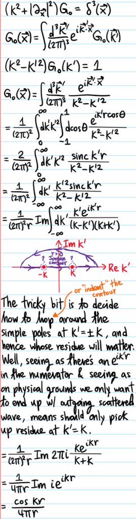
Problem #\(1\): Find the mistake in this derivation of the Green’s function for the inhomogeneous Helmholtz equation subject to the boundary condition of an outgoing wave:
Solution #\(1\): First of all, the correct answer should be \(G(r)=\frac{e^{ikr}}{4\pi r}\), not this standing wave with a \(\cos(kr)=(e^{ikr}+e^{-ikr})/2\) that superposes both an ingoing \(e^{-ikr}\) and outgoing wave \(e^{ikr}\). Reasoning that \(\cos(kr)\in\textbf R\) because it came after hitting with the \(\Im\) function, one might be led (correctly as it turns out) to the conclusion that this step:
was the seemingly innocuous but incorrect step. Basically, although it’s certainly true that \(\sin(k’r)=\Im e^{ik’r}\), the difficulty is that in order to be able to pull the \(\Im\) out of the integral, one has to be sure that the prefactor \(\frac{k’^2}{k^2-k’^2}\) is real. But in fact, despite looking very real, it should really have an \(i\varepsilon\) in the denominator (or sometimes just written as \(i0\) to reflect taking the limit \(\varepsilon\to 0\)). It is this slight shifting of the poles at \(k’=\pm k\) off the real axis to \(k’=\pm k\pm’i\varepsilon\) that makes this naive manipulation invalid!
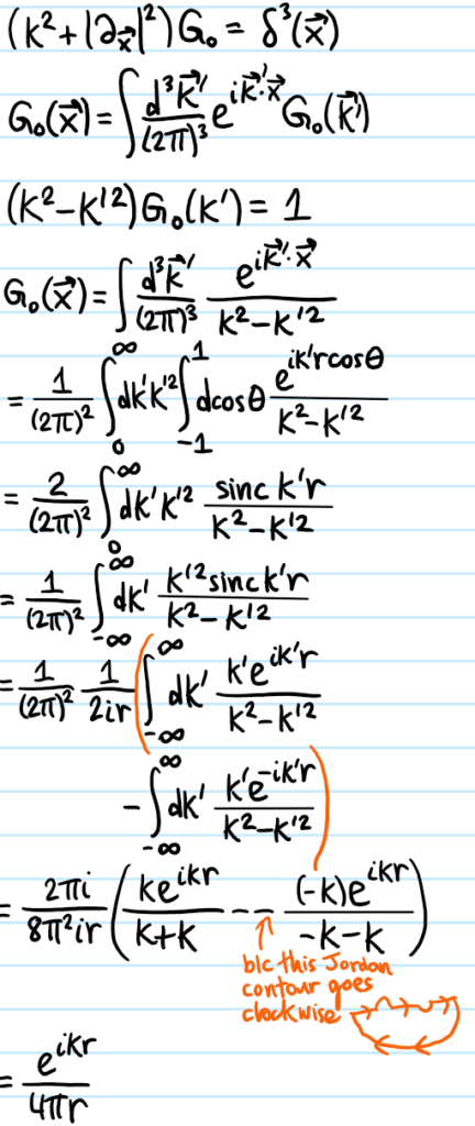
Problem #\(2\): Fix the mistake by redoing the derivation correctly
Solution #\(2\):
Problem #\(3\): Hence write down immediately the Lippman-Schwinger equation in the position representation for scattering off an arbitrary potential \(V\).
where the RHS is viewed as a \(\psi\)-dependent forcing function, so the solution of this inhomogeneous PDE is just the particular integral + complementary function:
Problem #\(4\): By aligning the incident momentum \(\textbf k=k\hat{\textbf z}\) along the \(z\)-axis and working asymptotically \(|\textbf x-\textbf x’|\approx |\textbf x|-\hat{\textbf x}\cdot\textbf x’\) in the exponent of the Green’s function \(G(r)=e^{ikr}/4\pi r\)while directly approximating \(|\textbf x-\textbf x’|\approx |\textbf x|\), obtain the Fraunhofer-Lippman-Schwinger equation:
Problem #\(5\): What is the scattering amplitude \(f(\hat{\textbf x})\) in the \(1^{\text{st}}\) Born approximation?
Solution #\(5\): Basically, just replace \(\psi(\textbf x’)\mapsto e^{i\textbf k\cdot\textbf x’}\) in the integrand (as that’s the plane wave solution when \(V=0\)). Thus, one finds that, up to some constants, the scattering amplitude \(f(\hat{\textbf x})\) in a given direction \(\hat{\textbf x}\) is determined by the Fourier structure of the potential \(V\), i.e. what is the amplitude of the plane wave in \(V\) travelling in the direction of the momentum transfer \(\textbf k’-\textbf k\):
Problem #\(7\): Apply the \(1^{\text{st}}\) Born approximation to calculate the Rutherford scattering amplitude \(f(\theta)\) in the cone \(\theta\) from a repulsive Coulomb potential.
Solution #\(7\): The Coulomb potential itself is not Fourier transformable, but the Yukawa potential \(V(r)=Ae^{-\kappa r}/r\) (which is like the Helmholtz Green’s function of a bound state?) has \(\hat V(k)=4\pi A/(k^2+\kappa^2)\) (no contour integration is even needed, this integral is very elementary). Then (nonrigorously) taking the limit \(\kappa\to 0\) (i.e. letting the range \(1/\kappa\to\infty\)) reproduces the Coulomb potential with supposed inverse-square Fourier transform \(\hat V(k)=4\pi A/k^2\). So the scattering amplitude in the \(1^{\text{st}}\) Born approximation is thus:
Problem: Show that the \(s\)-wave scattering amplitude \(f_s(k)\) is isotropic and related to the \(s\)-wave scattering length \(a_s\) of the isotropic potential \(V(r)\) by the Mobius transformation:
\[f_s(k)\approx-\frac{1}{ik+a^{-1}_s}=-a_s+ika_s^2+O(k^2)\to -a_s\text{ as }k\to 0\]
and hence as \(k\to 0\) the asymptotic wavefunction approaches \(\psi(r)\to 1-\frac{a_s}{r}\).
Solution: The partial wave expansion of the \(z\)-axisymmetric scattering amplitude \(f(\theta)\) in an isotropic potential \(V(r)\) receives contributions from all angular momentum sectors:
For low-energy \(k\to 0\) scattering, the \(\ell=0\) \(s\)-wave contribution dominates so that the scattering amplitude \(f(\theta)\approx f_0(k)P_0(\cos\theta)=f_0(k)=f_s(k)\) is not even a function of \(\theta\) anymore, i.e. it is isotropic!
In particular, in the low-energy limit \(k\to 0\) one has \(\delta_0(k)\to 0\) linearly as \(\delta_0(k)=-ka_s+O(k^2)\), so expanding \(\sin\delta_0(k)\approx\delta_o(k)\) and doing the slightly dodgy manipulation of writing \(e^{i\delta_0(k)}=\frac{1}{e^{-i\delta_0(k)}}=\frac{1}{1-i\delta_0(k)}\) one obtains the desired results. The asymptotic wavefunction is:
The purpose of this post is to review the classical theory of rigid body dynamics by working through a few illustrative problems in that regard.
Problem #\(1\): What defines a rigid body? What is an immediate corollary of this?
Solution #\(1\): A rigid body obeys \(|\textbf x_i-\textbf x_j|=\text{const}\) for all pairs of points \(i,j\) comprising the rigid body. As an immediate corollary, it follows that:
\[\frac{d}{dt}|\textbf x_i-\textbf x_j|^2=0\]
Writing \(|\textbf x_i-\textbf x_j|^2=(\textbf x_i-\textbf x_j)\cdot (\textbf x_i-\textbf x_j)\) and using the product rule leads one to an orthogonality criterion between the relative positions and velocities in a rigid body for all time:
Mathematically, this suggests that there should exist a single, universal vector \(\boldsymbol{\omega}\) called the angular velocity vector of the rigid body such that for all pairs \(i,j\) in the rigid body, one has:
Existence is always guaranteed, but one can find loopholes around uniqueness, e.g. the following rigid body consisting of a bunch of collinear point masses moving together with identical velocities \(\dot{\textbf x}_i=\dot{\textbf x}_j\) would admit any angular velocity \(\boldsymbol{\omega}\) along the line of their collinearity.
But in general, such situations never arise and so \(\boldsymbol{\omega}\) is unique at all times \(t\) (would be nice to obtain a rigorous proof of this intuition).
Problem #\(2\): How is the angular momentum \(\textbf L_{\textbf X}\) about a point \(\textbf X\) defined? What would it mean for \(\textbf X\) to be “fixed in some body frame” of a rigid body? Show that if \(\textbf X\) is fixed in some body frame, then the angular momentum \(\textbf L_{\textbf X}\) of the rigid body about \(\textbf X\) is:
i.e. inner product minus outer product. Note that \(\mathcal I_{\textbf X}^T=\mathcal I_{\textbf X}\) is clearly symmetric and positive semi-definite, so has \(3\) non-negative real eigenvalues \(I^1_{\textbf X},I^2_{\textbf X},I^3_{\textbf X}\) (for a given \(\textbf X\)) and orthogonal eigenspaces defining the so-called principal axes of the rigid body (with respect to \(\textbf X\)).
Solution #\(2\): The most useful definition in this context is:
The point \(\textbf X\) is said to be fixed in some body frame of a rigid body iff for all \(\textbf x_i\) comprising the rigid body, one has for all time \(|\textbf x_i-\textbf X|=\text{const}\); thus, if one likes one can think of \(\textbf X\) as just another mass element comprising the rigid body, except that it is massless.
In this case, it is clearly more desirable to work with the “fully relative” angular momentum \(\textbf L_{\textbf X}\) about \(\textbf X\) rather than the “partially relative” angular momentum \(\tilde{\textbf L}_{\textbf X}\) about \(\textbf X\) as it’s only in the former case that one can make use of the result \(\dot{\textbf x}_i-\dot{\textbf X}=\boldsymbol{\omega}\times(\textbf x_i-\textbf X)\) from Problem #\(1\) when \(\textbf X\) is fixed in some body frame:
where \(((\textbf x_i-\textbf X)\cdot\boldsymbol{\omega})(\textbf x_i-\textbf X)=(\textbf x_i-\textbf X)((\textbf x_i-\textbf X)\cdot\boldsymbol{\omega})=(\textbf x_i-\textbf X)((\textbf x_i-\textbf X)^T\boldsymbol{\omega})=((\textbf x_i-\textbf X)\textbf (\textbf x_i-\textbf X)^T)\boldsymbol{\omega}=(\textbf x_i-\textbf X)^{\otimes 2}\boldsymbol{\omega}\), so the result follows.
Problem #\(3\): Repeat Problem #\(2\) but for the kinetic energy \(T_{\textbf X}\) of a rigid body about a point \(\textbf X\) fixed in some body frame to show that:
Solution #\(3\): As always, it is essential to think in a clear-headed way about how various quantities are defined in the first place. In this case, there is no ambiguity (unlike the ambiguity between \(\textbf L_{\textbf X}\) and \(\tilde{\textbf L}_{\textbf X}\)), and one simply has:
In this case, \(|\dot{\textbf x}_i-\dot{\textbf X}|^2=|\boldsymbol{\omega}\times(\textbf x_i-\textbf X)|^2=|\boldsymbol{\omega}|^2|\textbf x_i-\textbf X|^2-(\boldsymbol{\omega}\cdot(\textbf x_i-\textbf X))^2=\boldsymbol{\omega}^T|\textbf x_i-\textbf X|^2\boldsymbol{\omega}-\boldsymbol{\omega}^T(\boldsymbol{\omega}\cdot(\textbf x_i-\textbf X))(\textbf x_i-\textbf X)\) and the rest is straightforward.
are true only for what point \(\textbf X\)? (note these decompositions are true not just for rigid bodies).
Solution #\(4\): Only when \(\textbf X\) coincides with the center of mass of the system as this ensures that cross-terms such as \(\sum_im_i(\textbf x_i-\textbf X)=\sum_im_i(\dot{\textbf x}_i-\dot{\textbf X})=\textbf 0\) vanish.
Problem #\(5\): Define the external torque \(\boldsymbol{\tau}_{\textbf X}^{\text{ext}}\) about \(\textbf X\) and, using this definition, check under \(2\) assumptions (which should be stated) that \(\dot{\textbf L}_{\textbf X}=\boldsymbol{\tau}_{\textbf X}^{\text{ext}}\) (again, this result is true not just for rigid bodies).
Solution #\(5\): The sensible definition in this case is:
Now the first assumption is that \(\textbf X\) coincides with the center of mass of the system. This allows the decomposition of \(\textbf L\) in Problem #\(4\) to be used, in particular:
Now comes the second assumption, namely that one is working in an inertial frame. This allows one to replace \(\dot{\textbf L}=\boldsymbol{\tau}^{\text{ext}}\) and \(M\ddot{\textbf X}=\textbf F^{\text{ext}}\). The claim follows.
Problem #\(5\): Synthesizing the results of the previous few problems, derive Euler’s equations for rigid body rotationabout the center of mass \(\textbf X\) in an inertial frame:
Solution #\(5\): The simple but important observation to make is that the center of mass \(\textbf X\) is also always fixed in any body frame (rigorous proof?). So conceptually, Euler’s equations are simply obtained by applying the product rule to:
except that it isn’t so obvious how to simplify \(\dot{\mathcal I}_{\textbf X}\) from its definition in Problem #\(2\). So instead, it will be convenient to choose a specific basis to carry out the computation in, and then revert back to the general vector notation. Specifically, the algebra is dramatically simplified in the principal body frame \((\hat{\textbf e}_1,\hat{\textbf e}_2,\hat{\textbf e}_3)_{\textbf X}\) with respect to which \(\mathcal I_{\textbf X}\) about the center of mass \(\textbf X\) is diagonal \(\mathcal I_{\textbf X}=\sum_{i=1}^3I_{\textbf X}^i\hat{\textbf e}_i^{\otimes 2}\) and moreover the principal moments of inertia \(I^1_{\textbf X},I^2_{\textbf X},I^3_{\textbf X}\) are \(t\)-independent. In this \(\mathcal I_{\textbf X}\)-eigenbasis, one can express \(\boldsymbol{\omega}=\sum_{i=1}^3\omega_i\hat{\textbf e}_i\) and hence \(\textbf L_{\textbf X}=\sum_{i=1}^3I^i_{\textbf X}\omega_i\hat{\textbf e}_i\), so applying the product rule gives:
Problem #\(6\): What does it mean for a rigid body to be free? Verify explicitly that both the kinetic energy \(T_{\textbf X}\) and magnitude of the angular momentum \(|\textbf L_{\textbf X}|\) are conserved for a free rigid body.
Solution #\(6\): A rigid body is said to be free iff it experiences no net external torque \(\boldsymbol{\tau}^{\text{ext}}_{\textbf X}=\textbf 0\) about its center of mass \(\textbf X\) in an inertial frame so that \(\textbf L_{\textbf X}\) is immediately conserved (and thus so is \(|\textbf L_{\textbf X}|\)). Moreover, because the inertia tensor is symmetric:
vanishes by virtue of dotting Euler’s equations with \(\boldsymbol{\omega}\).
Problem #\(7\): Describe Poinsot’s construction for visualizing the rotational dynamics of an arbitrary free rigid body.
Solution #\(7\): The idea is to first go to the principal body frame where one has (simplifying the notation on the principal moments of inertia a bit from earlier):
Thanks to Problem #\(6\), it follows that the angular velocity \(\boldsymbol{\omega}=\sum_{i=1}^3\omega_i\hat{\textbf e}_i\) is constrained to lie on a closed loop intersection of these two ellipsoids; it is common to visualize the first one (called the inertia ellipsoid) defined by the conserved kinetic energy \(T_{\textbf X}\) as embedded in the principal body frame of the rigid body so that the aforementioned closed loop on which \(\boldsymbol{\omega}\) travels is viewed as a trajectory (called the polhode) on the inertia ellipsoid.
So far this is just in the (principal) body frame, but in practice one is interested in how the rotation looks like in the inertial lab frame. For this, the key observation is that, reverting back to the vector notation, because \(T_{\textbf X}=\boldsymbol{\omega}\cdot\textbf L_{\textbf X}/2\) defines the equation of a plane in \(\boldsymbol{\omega}\)-space with normal vector \(\textbf L_{\textbf X}\), called the invariable plane; this also explains why one typically emphasizes the inertia ellipsoid over the “angular momentum ellipsoid”, since one thus has the nice interpretation that the inertia ellipsoid is tangent to the invariable plane at \(\boldsymbol{\omega}\), a fact which is confirmed by the gradient \(\partial T_{\textbf X}/\partial\boldsymbol{\omega}=\textbf L_{\textbf X}\) being orthogonal to contour surfaces. In the inertial lab frame, \(\boldsymbol{\omega}\) thus traces out a (not necessarily closed) trajectory called the herpolhode on the invariable plane as the inertia ellipsoid rolls without slipping on it (this is because, from the earlier rigid body kinematic formula \(\dot{\textbf x}_i-\dot{\textbf x}_j=\boldsymbol{\omega}\times(\textbf x_i-\textbf x_j)\), if one choose \(\textbf x_i\) to be the point of contact of the inertia ellipsoid with the invariable plane and \(\textbf x_j:=\textbf X\) the center of mass/center of the ellipsoid, then clearly \(\boldsymbol{\omega}\) is parallel to \(\textbf x_i-\textbf X\) and so the cross product vanishes, so \(\dot{\textbf x}_i=\dot{\textbf X}=\textbf 0\) which is the definition of rolling without slipping).
Another comment to make about Poinsot’s construction is that in some sense any free rigid body, no matter how jagged or complicated of an asteroid it is, can always be reduced to an ellipsoid with the same principal axes and moments of inertia; the \(2\) are kinematically indistinguishable but the latter has the advantage of being easier to interpret in terms of Poinsot’s construction. And clearly, understanding how the ellipsoid moves is equivalent to understanding how the principal axes of the original rigid body are rotating, which is all one could ask for to claim one has fully understood the dynamics of the rigid body!!! Systematically:
Step #\(1\): Mentally replace the rigid body by its inertia ellipsoid.
Step #\(2\): Figure out what the conserved \(\textbf L_{\textbf X}\) is; its magnitude determines the polhode on the inertia ellipsoid while its direction determines the invariable plane.
Step #\(3\): Keeping the invariable plane fixed in the lab frame, visualize the ellipsoid rolling without slipping on it along its polhode.
Step #\(4\): Now, optionally, get rid of the inertia ellipsoid as it was just a mental crutch and put the original rigid body back…but now it’s clear what it’s doing!
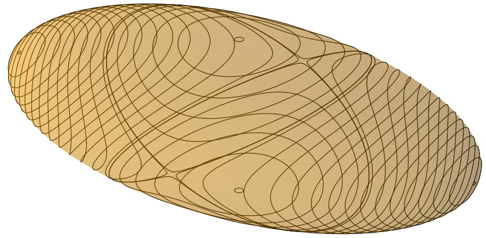
Here are some animations showing Poinsot’s construction for a particular free, asymmetric top with \(I_1\neq I_2\neq I_3\neq I_1\) varying the choice of \(\textbf L_{\textbf X}\), viewed in the lab frame
Problem #\(8\): State and explain intuitively the intermediate axis theorem (variously known as the tennis racket theorem or Dzhanibekov effect).
Solution #\(8\): For a free,asymmetric top (such as in the animations above), rotation about the principal axes \(\hat{\textbf e}_1\) and \(\hat{\textbf e}_3\) are stable, but rotation about \(\hat{\textbf e}_2\) is unstable. Although one can mathematically deduce it by linearizing, it also follows by inspecting the topology of the polhodes on the inertia ellipsoid for the asymmetric top (see also this nice qualitative explanation due to Terence Tao based on centrifugal force arguments in a rotating frame and video by Veritasium where it is explained that such a dramatic “flip” will not occur for the Earth by virtue of its non-rigidity which allows kinetic energy \(T_{\textbf X}\) to be dissipated internally as heat energy, thereby tending towards a minimal-energy state \(T_{\textbf X}=\sum_{i=1}^3L_i^2/2I_i\) of spinning about the principal axis with maximal moment of inertia).
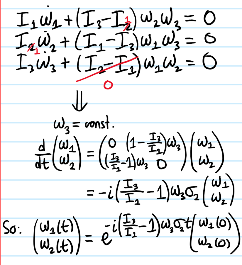
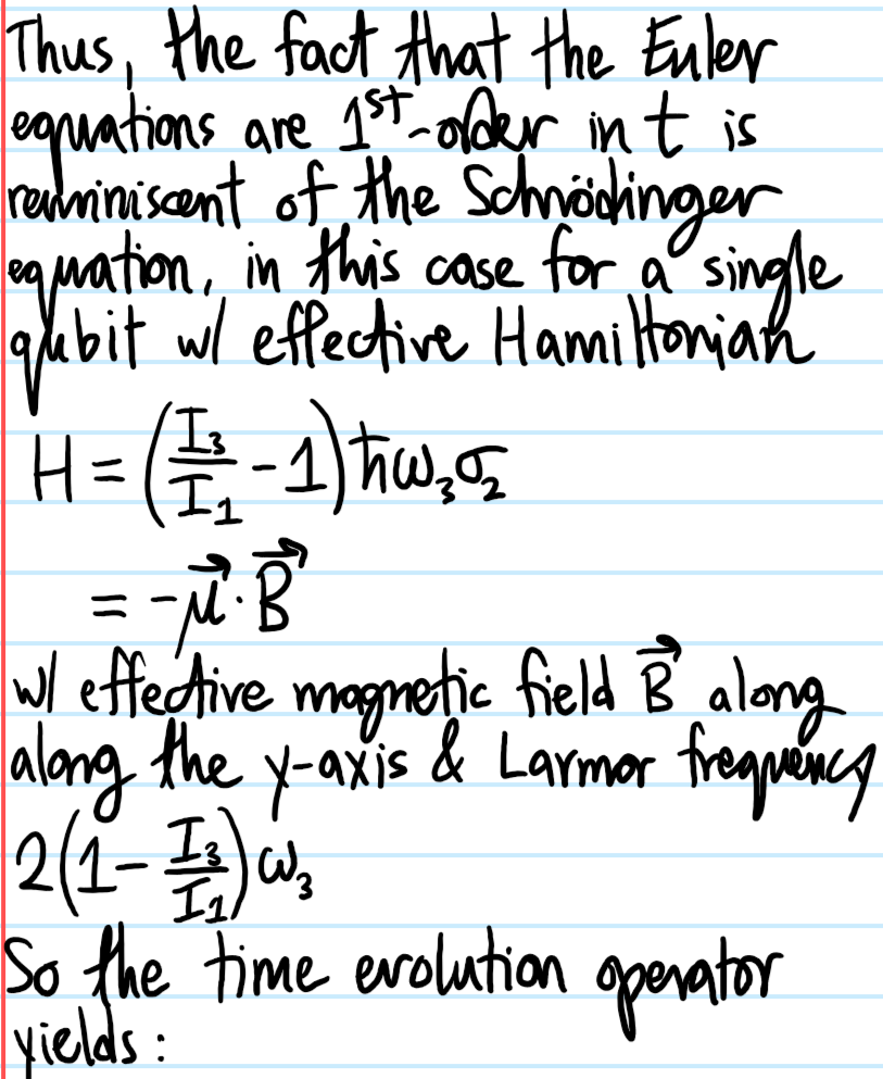
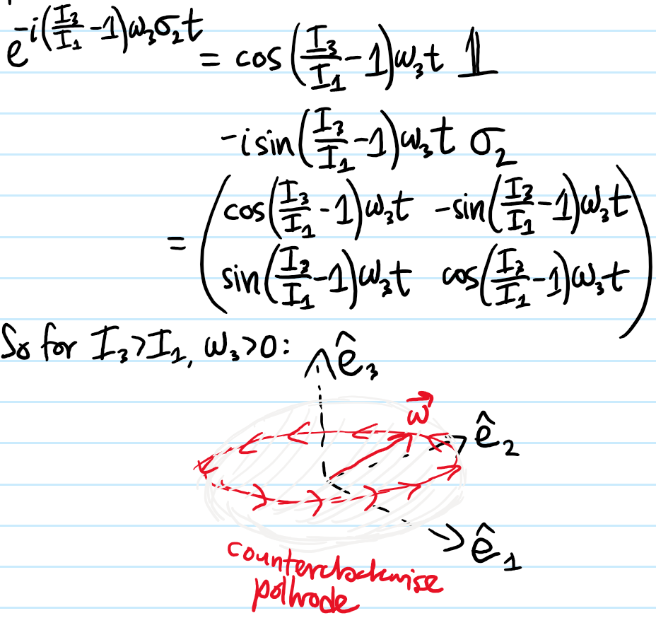
Problem #\(9\): Integrate Euler’s equations exactly for a free, symmetric top with \(I_1=I_2\).
Solution #\(9\):
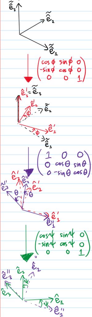
Problem #\(10\): Draw a diagram defining the Euler angles and rewrite Euler’s equations in terms of the Euler angles.
Solution #\(10\): The whole point of the Euler angles is to provide a language with which someone in the inertial lab frame can begin to talk about in a quantitative manner what the rigid body is doing (Poinsot’s construction with the herpolhode and all allows a good qualitative description but it doesn’t immediately offer anything quantitative).
Keep in mind there are many other (\(12\) to be precise) conventions for Euler angles. The \(SO(3)\) matrices should be interpreted not as active transformations of vectors in space, but as passive transformations of the basis which is why they look the way they do, for instance the last transformation says:
Problem #\(11\): In order to check that one has truly understood the Euler angles, explain what coefficient should replace each of the question marks in the linear combination below:
Problem #\(12\): Hence, how are the principal body frame angular velocities \((\omega_1,\omega_2,\omega_3)\) related to the Euler angles \((\phi,\theta,\psi)\)?
Solution #\(12\): Basically, one just needs to express \(\tilde{\hat{\textbf e}}_3\) and \(\hat{\textbf e}’_1 \) in the principal body frame. Although one can basically see the answer in the bottom row of that massive matrix above, in practice to rederive it the efficient way is to just walk directly from start to destination, i.e. in the first transformation \(\tilde{\hat{\textbf e}}_3=\hat{\textbf e}_3’\), in the next transformation \(\hat{\textbf e}_3’=\sin\theta\hat{\textbf e}_2^{\prime\prime}+\cos\theta\hat{\textbf e}_3^{\prime\prime}\) and in the last transformation \(\hat{\textbf e}_3^{\prime\prime}=\hat{\textbf e}_3\) while \(\hat{\textbf e}_2^{\prime\prime}=\sin\psi\hat{\textbf e}_1+\cos\psi\hat{\textbf e}_2\) so overall:
Solution #\(14\): Orienting the lab frame axes so that \(\textbf L\) lies along \(\tilde{\hat{\textbf e}}_3\), then by definition of the Euler angle \(\theta\) one has:
But both \(\textbf L\) and \(\omega_3\) are conserved for the free symmetric top, so \(\theta\) must also be conserved, i.e. \(\dot\theta=0\). This leads to the simplifications:
Rearranging leads to the desired \(\dot{\phi}=I_3\omega_3/I_1\cos\theta\). Finally, substituting this result into the remaining equation:
\[\omega_3=\dot{\phi}\cos\theta+\dot{\psi}\]
and isolating for \(\dot{\psi}=\left(1-\frac{I_3}{I_1}\right)\omega_3\) completes the proof.
Aside: one could also have started with the kinetic Lagrangian \(L=\frac{1}{2}I_1\dot{\phi}^2\sin^2\theta+\frac{1}{2}I_3(\dot{\phi}\cos\theta+\dot\psi)^2\), extracting the conserved momenta \(\partial L/\partial\dot{\phi},\partial L/\partial\dot{\psi}=I_3\omega_3\) and using the equation of motion \(\partial L/\partial\theta=0\) to quickly also obtain the results above.
Aside: a famous example of the free symmetric top considered by Richard Feynman is the case of a lamina (e.g. a plate) with \(I_1=I_2=I_3/2\) by the perpendicular axis theorem. Then in the lab frame, the precession/wobble rate \(\dot\phi\) and the spin rate \(\dot{\psi}\) are related by:
\[\dot{\phi}=-\frac{2\dot{\psi}}{\cos\theta}\]
In particular, when the nutation angle is very slight \(\theta\ll 1\), it follows that:
\[\dot{\phi}\approx -2\dot{\psi}\]
so the lamina wobbles twice as fast as it spins, for small inclinations.
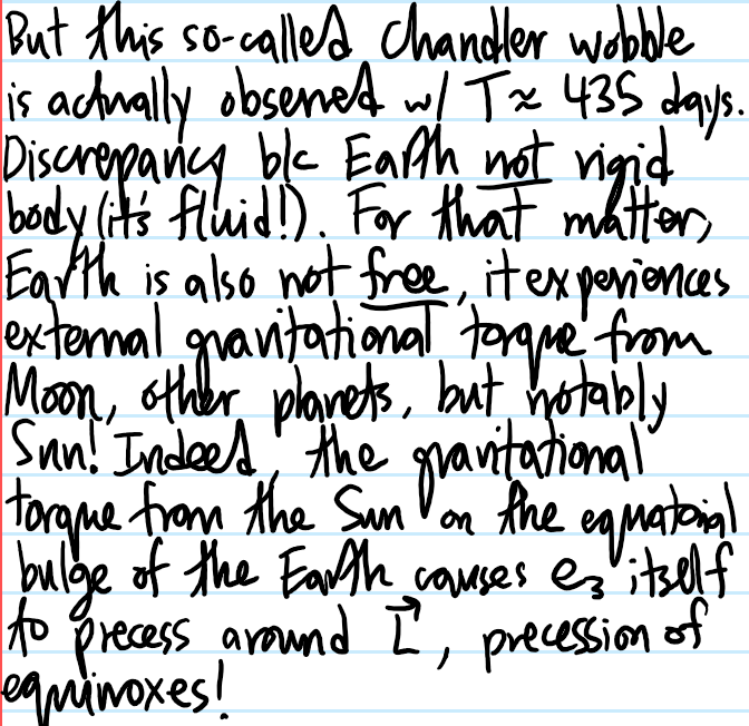
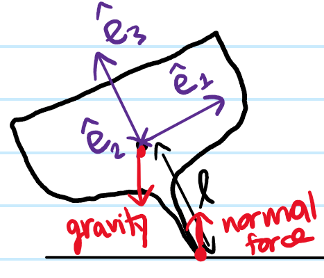
Problem #\(14\): The previous problems have all dealt with free rigid bodies. However, one can also consider a rigid body which is not free, being subject to an external torque \(\boldsymbol{\tau}_{\textbf X}^{\text{ext}}\). As an example, instead of a free symmetric top, consider a heavy symmetric top (e.g. a gyroscope) acted upon by a gravitational torque. Show that, just as there can be torque-free precession (Problem #\(9\)), there can also be torque-induced precession (in order to be able to do this problem, one absolutely requires the Euler angles in Solution #\(12\); thus, this just emphasizes again the point of Euler angles being to provide a language for discussing rigid body rotation in the lab frame).
Solution #\(14\):
The couple from gravity and the normal force is perfectly okay, but hard to express in the body frame? And also, I’m pretty sure the top will spin with its C.o.M fixed in the lab frame (rather than being pinned at the point of contact)? And as for the Lagrangian, just subtract \(-Mg\ell\cos\theta\), but \(\phi,\psi\) are still ignorable!
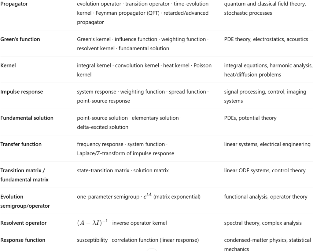
A ChatGPT thesaurus of all the synonyms of “propagator” across different disciplines:
Problem #\(1\): What is the retarded propagator of a quantum particle with Hamiltonian \(H\) in nonrelativistic quantum mechanics?
Solution #\(1\): At its heart, the “retarded” part should make one think of the causality factor \(\Theta(t-t’)\) while the “propagator” part should make one think of the time evolution operator \(\mathcal T\exp\left(-\frac{i}{\hbar}\int_{t’}^td\tilde t H(\tilde t)\right)\). So at its heart the retarded propagator is just the object:
\[\Theta(t-t’)\mathcal T\exp\left(-\frac{i}{\hbar}\int_{t’}^td\tilde t H\right)\]
that evolves states forward in time \(t\geq t’\). Indeed, the essence of this discussion holds for any kind of propagator in any context; they are basically just causal time evolution operators.
However, in the nonrelativistic (i.e. non-Lorentz invariant) quantum mechanics of a particle, one has access to its position observable \(\textbf X\) with position eigenstates \(|\textbf x\rangle\). So in this context, one may optionally (but conventionally) look at the matrix elements of the retarded propagator in the \(\textbf X\)-eigenbasis of that particle’s Hilbert space:
\[\Theta(t-t’)\langle\textbf x|\mathcal T\exp\left(-\frac{i}{\hbar}\int_{t’}^td\tilde t H\right)|\textbf x’\rangle\]
This now has the interpretation of the conditional probabilityamplitude for a measurement at time \(t\) of the particle’s position observable \(\textbf X\) to yield \(\textbf x\) given that at an earlier time \(t’\leq t\) the particle was prepared in a position eigenstate localized at \(\textbf x’\).
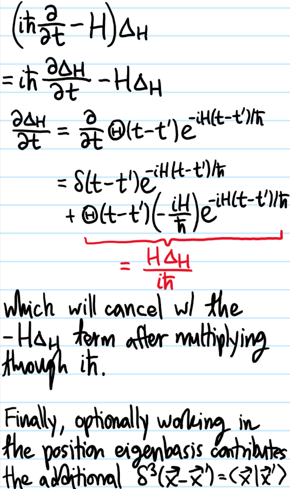
Problem #\(2\): Henceforth write \(U_H(t,t’):=\mathcal T\exp\left(-\frac{i}{\hbar}\int_{t’}^td\tilde t H\right)\) for the time evolution operator with respect to \(H\) so that \(i\hbar\dot U_H=HU_H\). Show that the retarded propagator is a retarded Green’s function for the Schrodinger operator \(\frac{\partial}{\partial t}-\frac{H}{i\hbar}\) in the sense that:
Solution #\(2\): The key fact is that the derivative of the step function \(\dot{\Theta}=\delta\) is a Dirac delta, which one can heuristically justify on the grounds that \(\Theta(t)=\int_{-\infty}^tdx\delta(x)\). Thus, when the \(\partial/\partial t\) operator hits the \(\Theta(t-t’)\), it will ultimately give the requisite \(\delta(t-t’)\) expected of any retarded Green’s function. The spatial \(\delta^3(\textbf x-\textbf x’)=\langle\textbf x|\textbf x’\rangle\) then arises as an artifact of working in the \(\textbf X\)-eigenbasis.
Problem #\(3\): Although not as relevant for nonrelativistic QM, one can also consider the advanced propagator:
Problem #\(3\): Hence, given any initial wavefunction \(\psi(\textbf x’,t’)\) at time \(t’\), how does the retarded propagator allow one to propagate this wavefunction forward in time to \(\psi(\textbf x,t)\) for \(t\geq t’\)?
Solution #\(3\): cf. Hugyen’s principle in wave optics:
Solution #\(2\): The nonrelativistic retarded propagator is intrinsic to the Hamiltonian \(H\) of the system, in particular being independent of whatever initial state \(|\psi(0)\rangle\) one prepares the particle in. More precisely, as the name “retarded propagator” suggests, its job is to propagate any initial state \(|\psi(0)\rangle\) forward in time by \(t>0\) (remember again that at its essence it’s just a causal time evolution operator!). That is, for \(t>0\) one can just set \(\Theta(t)=1\) and by insert a resolution of the identity:
Emphasizing again, the \(\textbf x\) and \(\textbf x’\) are very much the unimportant labels in that equation; the causal time evolution of the state \(|\psi(0)\rangle\mapsto|\psi(t)\rangle\) is at the heart of the retarded propagator.
Problem #\(3\): Show that the nonrelativistic retarded propagator \(\Delta_H(t’,\textbf x’|t,\textbf x)\) is a retarded Green’s function for the Schrodinger operator:
and using the plane wave momentum eigenstate \(\langle\textbf x|\textbf p\rangle=e^{i\textbf p\cdot\textbf x/\hbar}/(2\pi\hbar)^{3/2}\), this can be shown to reduce to (after performing the relevant Gaussian integrals):
Thus, roughly speaking, the propagator of a free particle at \(t=0\) is infinitely peaked at \(\textbf x=0\) but broadens over time \(t\) into an isotropic Gaussian with “imaginary” radial width \(\sigma_{|\textbf x|}=\sqrt{i\hbar t/m}\) exhibiting the usual \(\propto\sqrt{t}\) diffusion with “quantum diffusivity” \(D=i\hbar/m\).
Problem: Using Fourier transforms, calculate the Green’s function for the operator \(i\hbar\frac{\partial}{\partial t}-\frac{|\textbf P|^2}{2m}\) and by taking an inverse Fourier transform, show explicitly that it agrees, up to a factor of \(i\hbar\) with the propagator above.
Solution: The Green’s function in \(\textbf k,\omega\)-space is a simple Mobius transformation:
So the purpose of the pole at \(\omega=\omega_k=\hbar k^2/2m\) is to ensure that when using Cauchy’s integral formula in this inverse FT, the particle is put on-shell with that dispersion. Doing the Gaussian integrals then reproduces \(1/i\hbar\) times the propagator.
Problem #\(6\): Repeat Problem #\(5\) but for the \(1\)-dimensional quantum harmonic oscillator of trapping frequency \(\omega\). Hence, deduce the identity of Hermite polynomials:
Newton’s second law in its most basic form states that for a single point mass, \(\dot{\textbf p}=\textbf F\) in any inertial frame. Combining this with Newton’s third law (antisymmetry of forces \(\textbf F_{i\to j}=-\textbf F_{j\to i}\), similar to many other antisymmetric phenomena in physics such as relative velocities \(\textbf v_{ij}=-\textbf v_{ji}\)) gives the most useful system formulation of Newton’s second law \(\dot{\textbf P}=\textbf F^{\text{ext}}\) in any inertial frame where \(\textbf P:=\sum_{i=1}^N\textbf p_i\) is the total momentum of a system of \(N\) point masses.
For the single-particle form \(\dot{\textbf p}=\textbf F\) of Newton’s second law, crossing both sides with the particle’s position \(\textbf x\) (relative to any origin, stationary, moving, accelerating, etc. as seen in the inertial frame) gives \(\dot{\textbf L}=\boldsymbol{\tau}\) in any inertial frame (this is thanks to a combination of two facts, namely: the cross product is a derivation, and it is non-degenerate, I wonder if there is a theory which generalizes this observation?) a rotational analog of Newton’s second law. Thus, naturally one might hope that an analog \(\textbf L=\boldsymbol{\tau}^{\text{ext}}\) should hold at the system level too, with \(\textbf L=\sum_{i=1}^N\textbf L_i\) and \(\boldsymbol{\tau}^{\text{ext}}=\sum_{i=1}^N\boldsymbol{\tau}^{\text{ext}}_i\). This identity is indeed true provided that the angular momenta \(\textbf L_i\) and external torques \(\boldsymbol{\tau}^{\text{ext}}_i\) are all measured in an inertial frame relative to a point \(\tilde{\textbf X}\) moving parallel at all times to the center of mass \(\textbf X\) of the system. The proof is a direct computation:
Now, the idea is to decompose the forces on each particle as \(\textbf F_i=\textbf F^{\text{ext}}_i+\sum_{j=1}^N\textbf F_{j\to i}\) with the non-degenerate \(\textbf F_{i\to i}=\textbf 0\). This finally gives:
where \(\boldsymbol{\tau}^{\text{int}}=\sum_{1\leq i<j\leq N}(\textbf x_i-\textbf x_j)\times\textbf F_{j\to i}\) are \(N\choose 2\)\(=\frac{N(N-1)}{2}\) internal, reference-independent couples (and one would normally use one’s intuition to think about these rather than explicitly appealing to the formula) and \(\boldsymbol{\tau}^{\text{ext}}=\sum_{i=1}^N(\textbf x_i-\tilde{\textbf X})\times\textbf F^{\text{ext}}_i\). So it is clear that in order to have \(\dot{\textbf L}=\boldsymbol{\tau}^{\text{ext}}\) there are two obstacles in the way. Although actually, one of them is always zero, namely the internal couples \(\boldsymbol{\tau}^{\text{int}}=\textbf 0\). This follows from Galilean covariance (rather than from God, as my high school physics teacher told me); forces at a distance like gravity, electrostatics, masses pulled by springs or tension forces through ropes all have to be central (and thus conservative) so the cross product vanishes. On the other hand, the only time one can achieve an azimuthal/tangential/angular component of force is with friction, but then friction is not a force at a distance, but is rather a contact force and so the relative position \(\textbf x_i-\textbf x_j=\textbf 0\) at the point of transmission (the normal force is thus also zero because it simultaneously falls into both of those categories). I suspect any force of only position has to be like this, velocity-dependent forces like the magnetic force may be more subtle depending on Newtonian vs. relativistic frameworks, etc. To zero the remaining obstacle, since \(\textbf P=M\dot{\textbf X}\), it is both sufficient and necessary to have \(\tilde{\textbf X}||\textbf X\) at all times as claimed (e.g. a common, but certainly not the only choice is \(\tilde{\textbf X}:=\textbf X\)).
For instance, consider a hollow cylinder rolling without slipping down a ramp (couched in some inertial frame obviously). Take \(\tilde{\textbf X}\) to be the point of contact of the wheel with the ramp (clearly not associated with any physical particle). However, because \(\tilde{\textbf X}\) clearly moves parallel to \(\textbf X\) (indeed, it moves with the exact same velocity, just displaced from it), we know that \(\dot{\textbf L}=\boldsymbol{\tau}^{\text{ext}}\) relative to \(\tilde{\textbf X}\). Since this particular system of particles is in fact a rigid body, it is convenient to work with their common \(\omega\) and so \(L=I\omega\) (this step only works because of rolling without slipping) where by the parallel axis theorem \(I=2MR^2\). Now, one convenience of choosing \(\tilde{\textbf X}\) as the point of contact is that all contact forces acting at \(\tilde{\textbf X}\) by definition exert no torque about \(\tilde{\textbf X}\). So the only one is gravity. This yields \(\dot{\omega}=\frac{g\sin(\theta)}{2R}\). Since \(\omega\) is the same about any point (still don’t have very good intuition for this fact), one can do the derivation choosing \(\tilde{\textbf X}:=\textbf X\) instead, but it will be more lengthy since one has to more explicitly invoke the rolling without slipping constraint and Newton’s second law in its translation form to eliminate the static friction enforcing the rolling without slipping. The result is the same however, giving credence to the method.
My first year Cambridge physics supervisor also showed me a cute way to think about the situation which is mathematically equivalent to the above but conceptually somewhat different. The thing is that Newton’s second law refers only to a vector addition of force vectors, with no regards for where the point of application of those forces is (clearly if one is only interested in the center of mass motion, it doesn’t matter!). The torques are the devices that are sensitive to the point of application. So the idea is to basically draw the free body diagram of a system. Then, any forces that are not acting at the center of mass, draw a fictitious copy of the force acting at the center of mass but then to balance this out draw its negation also acting at the center of mass (if it acted elsewhere it wouldn’t affect the CoM motion but definitely the rotational dynamics!). Do this for all forces not acting at the CoM. The final result is that the torque about the CoM is completely comprised of reference-independent couples which dramatically clarifies the situation. Meanwhile, there is a unbalanced force left acting on the center of mass, which, intuitively, dictates its motion by Newton’s second law (actually, all this discussion holds equally well with CoM replaced by \(\tilde{\textbf X}\)). Hopefully this discussion will help me go back to learn rigid body dynamics more carefully and understand better.
The purpose of this post is to appreciate that the familiar idea of non-interacting particles from e.g. statistical mechanics manifests in the context of QFT as a free quantum field theory.
Problem #\(1\): What defines a free classical field theory? Give an example.
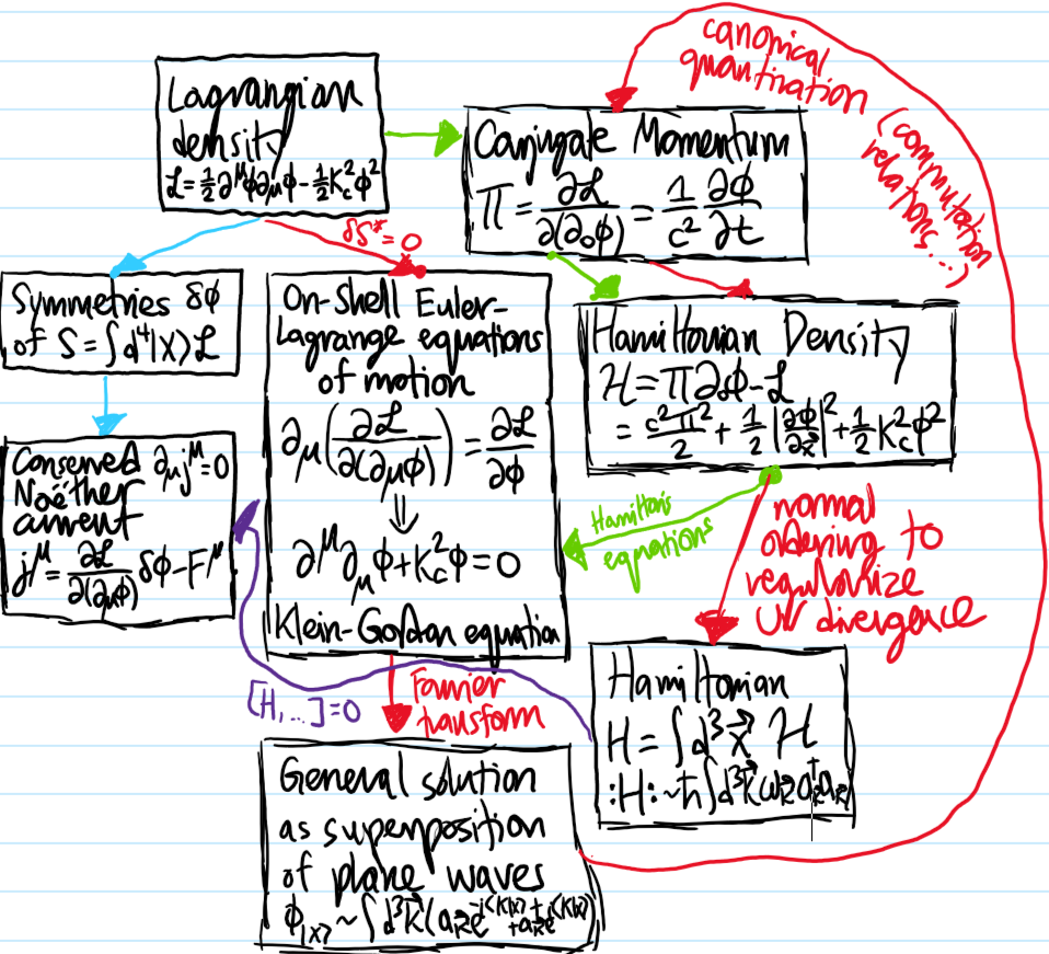
Solution #\(1\): A classical field theory is said to be free iff its Lagrangian density \(\mathcal L\), or equivalently Hamiltonian density \(\mathcal H\), is quadratic in all fields \(\phi_i\). Why? Because the corresponding Euler-Lagrange equations of motion for the fields \(\phi_i\) would then be linear in the \(\phi_i\). An example of a free classical field theory is the classical Klein-Gordon field theory which governs just a single, relativistic, real scalar field \(\phi(X)\):
(aside: Klein-Gordon field theory is “relativistic” in the sense of being Lorentz-invariant as manifest from the Lagrangian density \(\mathcal L\). It is “real” \(\phi(X)\in\textbf R\) because, when canonically quantized, it turns out to only give rise to neutral particles. It is clearly free. And it is a scalar field (as opposed to a vector field like in E&M) because, again when canonically quantized from a CFT to a QFT, turns out to also only describe spinless \(s=0\) bosons). Think Higgs boson for instance.
Problem #\(2\): In the context of the quantum harmonic oscillator from non-relativistic particle mechanics, the operators \(a,a^{\dagger}\) are typically called lowering and raising operators respectively. In moving from quantum particles to quantum fields however, the key conceptual leap that the number of particles is not conserved gives rise to an entirely new perspective on what \(a,a^{\dagger}\) are so that in QFT they are called annihilation and creation operators.
But, first, just using “classical cheating”, define \(a\) and \(a^{\dagger}\) and compute their commutator \([a,a^{\dagger}]\). Also define the number operator \(N\) and compute \([N,a]\) and \([N,a^{\dagger}]\).
Solution #\(2\): By inspecting the classical Hamiltonian:
\[H(x,p)=\frac{p^2}{2m}+\frac{m\omega^2x^2}{2}\]
One can construct a characteristic quantum oscillator length \(x_0\) and oscillator momentum \(p_0\) through the virial relations:
This sum of squares suggests the classical factorization:
\[H=\hbar\omega N\]
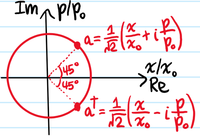
where \(N:=aa^{\dagger}\) and the isomorphism \(\cong\) between phase space \(\textbf R^2\) and the complex plane \(\textbf C\) is exploited:
Since canonical quantization is a Lie algebra representation up to quadratic polynomials on phase space (which applies to everything here), it follows that all Poisson bracket computations must agree with the corresponding commutators. In particular:
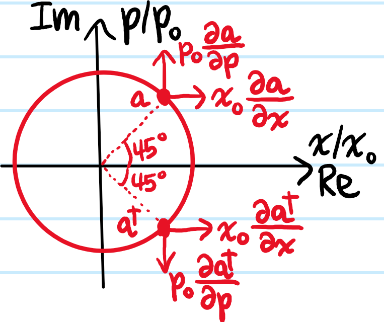
\[\{a,a^{\dagger}\}=\det\begin{pmatrix}\partial a/\partial x&\partial a^{\dagger}/\partial x \\ \partial a/\partial p & \partial a^{\dagger}/\partial p\end{pmatrix}=-\frac{i}{x_0p_0}=\frac{1}{i\hbar}\]
which could also be obtained just from drawing pictures like:
This “proves” that \([a,a^{\dagger}]=i\hbar\{a,a^{\dagger}\}=1\). The other commutators can be quickly obtained using the “product rule” for Poisson brackets:
(note that although \([F,G]^{\dagger}=[G^{\dagger},F^{\dagger}]\) for commutators, for Poisson brackets it’s just \(\{f,g\}^{\dagger}=\{f^{\dagger},g^{\dagger}\}\)).
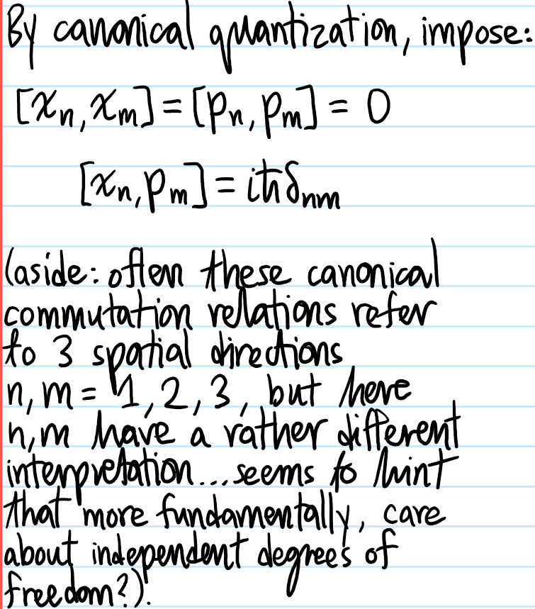
Problem #\(3\): A \(1\)D string has Hamiltonian density:
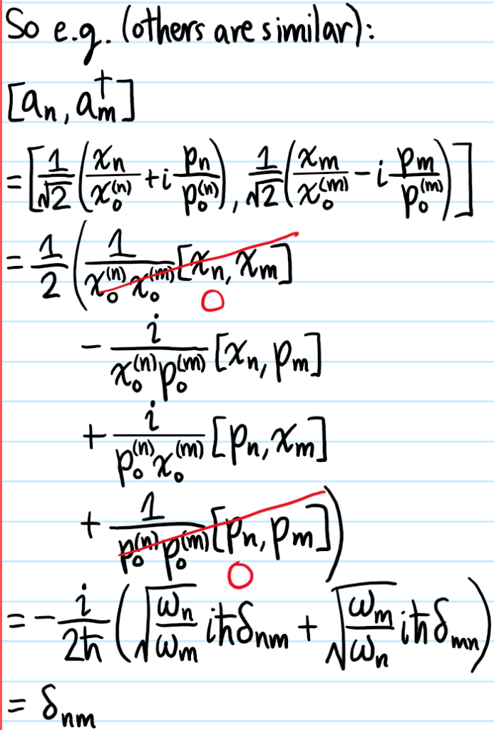
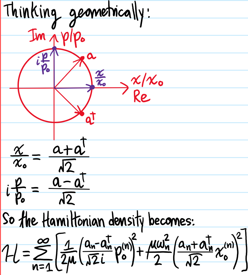
Unlike the previous problem where there was just \(1\) harmonic oscillator, here there are an infinite number of harmonic oscillators, one for each normal mode \(n=1,2,3,…\) (however, here it is only countably infinite; in QFT it will often be uncountably infinite!). Thus, each one gets its own pair of creation and annihilation operators \(a_n,a_n^{\dagger}\) defined analogously as in Problem #\(2\) (but where each oscillator now also has its own characteristic length \(x_0^{(n)}=\sqrt{\hbar/\mu\omega_n}\) and characteristic momentum \(p_0^{(n)}=\sqrt{\hbar\mu\omega_n}\)). Check that for distinct oscillators \(n\neq m\), these operators don’t talk to each other in the sense that \([a_n,a_m]=[a_n^{\dagger},a_m^{\dagger}]=0\) and \([a_n,a_m^{\dagger}]=\delta_{nm}\). Show that the Hamiltonian density can be rewritten:
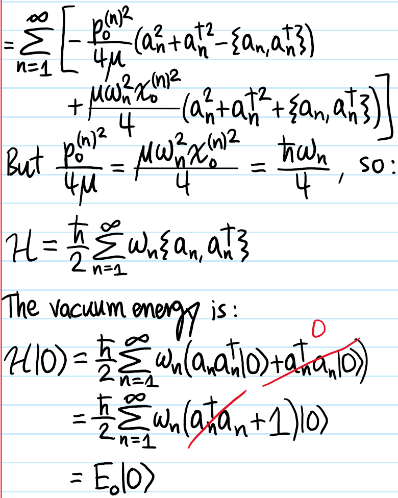
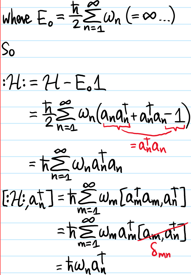
Assuming there exists a single universal ground state \(|0\rangle\) annihilated by \(a_n|0\rangle=0\) for all \(n=1,2,3,…\), show that, after discarding the vacuum energy, \(\mathcal H\mapsto :\mathcal H:\) takes the normally ordered form:
Substituting this as an ansatz into the Klein-Gordon equation yields, for each \(\textbf k\in\textbf R^3\), the equation of motion of a simple harmonic oscillator for \(\hat{\phi}(\textbf k,t)\):
(defined here as the positive square root). So the most general solution in \(\textbf k\)-space is parameterized by two arbitrary scalar fields \(a_{\textbf k},b_{\textbf k}\):
However, demanding that \(\phi(\textbf x,t)\) be a real scalar field so that \(\phi^{\dagger}(\textbf x,t)=\phi(\textbf x,t)\) (which is equivalent to demanding that its Fourier transform be Hermitian \(\hat{\phi}^{\dagger}(\textbf k,t)=\hat{\phi}(-\textbf k,t)\)) forces \(b_{\textbf k}=a_{-\textbf k}^{\dagger}\). Thus actually one can simply write:
Or, defining the four-wavevector \(|K\rangle:=(\omega_{\textbf k}/c, \textbf k)\), working with the standard four-position \(|X\rangle:=(ct,\textbf x)\), and using the time-like convention for the Minkowski metric \(\eta=\text{diag}(1,-1,-1,-1)\):
Note here that one is still working entirely within the realm of classical field theory (not QFT yet!) so the daggers \(\dagger\) are nothing more than complex conjugation, and in particular \(\phi(X)\) is a (real) scalar field rather than a (Hermitian) operator field. This is similarly the case with \(a_{\textbf k},a_{\textbf k}^{\dagger}\) being (complex) scalar fields at this stage rather than operator fields. Finally, it is worth noting that the conjugate real scalar momentum field is:
Problem #\(6\): Explain what it means to take the classical Klein-Gordon theory governing the real scalar fields \(\phi(X),\pi(X)\) and canonically quantize them in the Heisenberg picture to Hermitian operator fields, thereby constructing a free quantum Klein-Gordon field theory. What changes in the Schrodinger picture?
Solution #\(6\): On paper, the equations are invariant. Canonical quantization is really more of a conceptual leap, in that the fundamental “data type” of the objects in the equations are what changes. Specifically, one now promotes \(\phi(X),\pi(X)\) to operator fields, i.e. a function associating an operator to each event \(|X\rangle\) in Minkowski spacetime. It follows that the only way the classical Klein-Gordon field decompositions in the Fourier basis of plane waves can be compatible with canonical quantization is iff, in addition to promoting \(\phi(X),\pi(X)\) to operator fields, one also/simultaneously promotes the “Fourier coefficients” \(a_{\textbf k},a_{\textbf k}^{\dagger}\) to operators.
Furthermore, it turns out one should postulate equal-\(t\) commutation relations between these operators in the Heisenberg picture:
though one can show through straightforward computations in the spirit of Problem #\(5\) that these are logically equivalent to the following commutation relations on the Fourier coefficients (cf. Problem #\(3\)):
where the isotropy of the dispersion relation \(\omega_{-\textbf k}=\omega_{\textbf k}=\omega_{|\textbf k|}\) has been used. The expression for \(\hat{\phi}(\textbf k,t)\) was already given above, but can also of course be recovered by identical manipulations. So, in analogy with the classical case in Problem #\(3\), one has:
which are happily consistent with each other (note also that \(a_{\textbf k}\) is \(t\)-independent so all \(t\)-dependence on the right-hand side is spurious). One then has e.g.
But the commutation relations postulated on \(\phi(\textbf x,t)\) and \(\pi(\textbf x,t)\) in real space directly imply their corresponding commutation relations in \(\textbf k\)-space, for instance:
\[=\frac{i\hbar}{(2\pi)^3}\int d^3\textbf x e^{i(\textbf k’-\textbf k)\cdot\textbf x}=i\hbar\delta^3(\textbf k-\textbf k’)\]
From here the result follows. In a way, the fact that it is equal-\(t\) commutators of the operator fields which appear could be construed as motivation for imposing equal-\(t\) commutation relations in the first place. One can of course also easily show the converse, i.e. that imposing the commutation relations on \(a_{\textbf k},a_{\textbf k}^{\dagger}\) yield those of \(\phi\) and \(\pi\).
Problem #\(7\): Calculate the Hamiltonian \(H=\int d^3\textbf x\mathcal H\) for the free Klein-Gordon quantum field theory. In particular, comment on the infrared and ultraviolet divergences present and how one can regularize them.
Using the relativistic dispersion relation \(\omega_{\textbf k}^2/c^2=|\textbf k|^2+k_c^2\), the \(t\)-dependent oscillatory terms vanish and one finds that:
However, even after this replacement the second term still goes like \(\sim\int d^3\textbf k\omega_{\textbf k}=\infty_{\text{UV}}\) which diverges when integrated over \(\textbf k\in\textbf R^3\); it is called an ultraviolet divergence. In this case, it turns out one can deal with it by just subtracting it off from \(H\) (note it can also be interpreted as the zero-point energy \(E_0\) of the vacuum state \(|0\rangle\)) to obtain:
though the Casimir force and cosmological constant are \(2\) cases where this cannot be done.
Pragmatically speaking, normal ordering allows one to commute creation and annihilation operators with impunity (no need to worry about IR or UV divergences), i.e. \(:[a_{\textbf k},a_{\textbf k’}^{\dagger}]:=0\).
Problem #\(8\): Show that \([:H:,a_{\textbf k}^{\dagger}]=\hbar\omega_{\textbf k}a_{\textbf k}^{\dagger}\) and \([:H:,a_{\textbf k}]=-\hbar\omega_{\textbf k}a_{\textbf k}\) are identical to the classical results in Problem #\(3\). Hence, explain how excited states of the free quantum field \(\phi\) can be interpreted as identical spinless bosons.
and taking its adjoint yields the other commutation relation. Hence, one can declare victory; the excited state \(a_{\textbf k}^{\dagger}|0\rangle\) may be checked to be an \(:H:\)-eigenstate:
with energy \(E_{\textbf k}:=\hbar\omega_{\textbf k}\) above the ground state energy \(E_{\textbf 0}=0\). This already provides some evidence for the particle interpretation
As further evidence, one can check that the excited state \(a_{\textbf k}^{\dagger}|0\rangle\) has momentum \(\textbf p_{\textbf k}=\hbar\textbf k\) just like for a particle. To see this, note that for Klein-Gordon theory the energy-momentum tensor is symmetric with:
where the momentum density is \(\boldsymbol{\mathcal P}=-\frac{1}{c^2}\frac{\partial\phi}{\partial t}\frac{\partial\phi}{\partial\textbf x}\) from which one obtains the conserved momentum \(\textbf P:=\int d^3\textbf x\boldsymbol{\mathcal P}\):
which includes contributions from both orbital angular momentum and spin angular momentum \(\textbf J=\textbf L+\textbf S\). In particular, if one artificially fixes \(\textbf L=\textbf 0\) by considering a stationary particle \(|\textbf k=\textbf 0\rangle=a_{\textbf k=\textbf 0}^{\dagger}|0\rangle\), then this has:
\[\textbf J|\textbf k=\textbf 0\rangle=0\]
so the particles that arise as excitations of the free quantum field are spinless as mentioned earlier. Furthermore, given any multi-particle excited state:
the exchange of any two particles \(\textbf k_1\leftrightarrow\textbf k_2\) yields a physically equivalent state (since all creation operators commute) so these are by definition identical bosons.
As an aside, this particle interpretation of the excited states is also what justifies calling the ground state \(|0\rangle\) as the “vacuum state” because classically a vacuum is thought of as containing no particles.
Problem #\(9\): What is the state space \(\mathcal F\) of the free Klein-Gordon quantum field theory?
Solution #\(9\): It is known as Fock space, and is just the direct sum of all \(N\)-particle sectors \(\mathcal F_N=\text{span}_{\textbf C}\{\prod_{i=1}^Na_{\textbf k_i}^{\dagger}|0\rangle:\textbf k_i\in\textbf R^3\}\):
\[\mathcal F:=\oplus_{N=0}^{\infty}\mathcal F_N\]
It is denoted by \(\mathcal F\) rather than \(\mathcal H\) to avoid confusion with the Hamiltonian density (cf. in statistical mechanics where, to specify the microstate of a Bose gas, one just has to specify Bose occupation numbers in each single-boson state; this is the Fock space at work).
Problem #\(10\): Define the number operator \(N\), explain what it does, and check that it commutes with \(:H:\); what is the implication of this for free quantum field theories?
Solution #\(10\): It takes the normally ordered form:
And it is easy to convince oneself that \(N|\textbf k_1,\textbf k_2,…,\textbf k_n\rangle=n|\textbf k_1,\textbf k_2,…,\textbf k_n\rangle\) counts the number \(n\) of spinless bosons in a given multi-boson state \(|\textbf k_1,\textbf k_2,…,\textbf k_n\rangle\in \mathcal F_n\). Finally:
so the number of particles in free field theories are conserved (a property which is decisively not true of interacting field theories).
Problem #\(11\): Show that the neither the state \(a_{\textbf k}^{\dagger}|0\rangle\) nor \(\phi(\textbf x,t)|0\rangle\) are normalizable in \(\mathcal F\).
Solution #\(11\): Assuming the vacuum state is normalized \(\langle 0|0\rangle=1\), then for the single-boson excitation \(|\textbf k\rangle=a_{\textbf k}^{\dagger}|0\rangle\), one picks up the same IR divergence as before:
Similarly, although \(\langle 0|\phi(\textbf x,t)|0\rangle=0\), the fluctuations of \(\phi\) at a fixed event \((\textbf x,t)\) (which is also the norm-squared of the state since \(\phi^{\dagger}=\phi\)):
Problem #\(12\): Outline why \(\int\frac{d^3\textbf k}{\omega_{\textbf k}}\) is Lorentz invariant. Hence, define a relativistically “normalized” one-particle Fock state \(|\textbf k\rangle\).
Solution #\(12\): Clearly the measure \(d^4|K\rangle\) is Lorentz invariant (more precisely, \(SO(1,3)\)-invariant since \(|K’\rangle=\Lambda|K\rangle\) gives a Jacobian determinant \(\det\frac{\partial|K’\rangle}{\partial|K\rangle}=\det\Lambda=1\) for \(\Lambda\in SO(1,3)\)) and the inner product \(\langle K|K\rangle=\frac{\omega^2}{c^2}-|\textbf k|^2\) is also Lorentz invariant (this time \(O(1,3)\)-invariant), and finally the step function \(\Theta(\omega)\) is also Lorentz invariant (this time \(O^+(1,3)\)-invariant), so all in all, when the measure \(d^4|K\rangle\) is integrated on the mass shell \(\langle K|K\rangle=k_c^2\) and with the condition \(\omega>0\):
the resulting object must be Lorentz invariant (i.e. \(SO^+(1,3)\)-invariant). Note that the identity \(\delta^n(\textbf F(\textbf x))=\sum_{\textbf x_0\in\textbf R^n:\textbf F(\textbf x_0)=\textbf 0}\frac{\delta(\textbf x-\textbf x_0)}{|\det\frac{\partial\textbf F}{\partial\textbf x}(\textbf x_0)|}\) has been used.
Therefore, if one works with the following relativistic normalization for the Fock states:
Problem #\(13\): Recall that when canonically quantizing the classical free Klein-Gordon field theory for a real scalar field in the Hamiltonian formulation, the canonical commutation relations in the Heisenberg picture were equal-\(t\) commutators. For instance, at an equal time \(t\) and for any two distinct locations in space \(\textbf x\neq\textbf x’\), the operators \(\phi(\textbf x,t),\phi(\textbf x’,t)\) associated to the space-like separated events \((ct,\textbf x),(ct,\textbf x’)\) were postulated to commute:
\[[\phi(\textbf x,t),\phi(\textbf x’,t)]=0\]
However, in order for the theory to be compatible with special relativity, and in particular causality, it must be the case that:
\[[\phi(X),\phi(X’)]=0\]
for any two space-like separated events \(|X-X’|^2<0\) outside each other’s light cones, not just for two simultaneous events. Despite not being manifest, show that this is indeed the case.
Solution #\(13\): By directly chugging in the Fourier mode expansion for \(\phi\), one finds that the commutator is simply proportional to the identity in this free QFT (cf. many other commutators like \([X,P_x]=i\hbar 1\) and \([a,a^{\dagger}]=1\) in quantum mechanics where this occurs, so commonly that it is sometimes called a “c-number function” where the “c” stands for “classical”):
The fact that the integrand involves only the Lorentz invariant inner product \(\langle K|X-X’\rangle\) and that the measure \(\int d^3\textbf k/\omega_{\textbf k}\) is Lorentz invariant (thanks to Solution #\(12\)), it follows that the c-number commutator is also Lorentz invariant, i.e. for any \(\Lambda\in SO^+(1,3)\), \([\phi(\Lambda^{-1}X),\phi(\Lambda^{-1}X’)]=[\phi(X),\phi(X’)]\). Now, let \(|X-X’|^2<0\) be spacelike separated events. Then, and this is the key insight, there exists some Lorentz transformation \(\Lambda\in SO^+(1,3)\) such that \(\Lambda X\) and \(\Lambda X’\) become simultaneous events, so write \(\Lambda X-\Lambda X’=(0,\Delta\textbf x)\). But this then reproduces the originally postulated equal-\(t\) commutation relation:
since the integrand \(\sim\sin(\textbf k\cdot\Delta\textbf x)\) is odd in \(\textbf k\). Thus, causality is preserved.
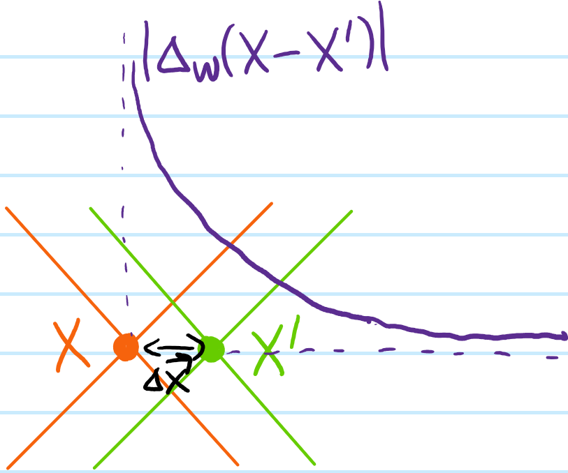
Problem #\(14\): Define the Wightman propagator of Klein-Gordon free QFT to be the two-point correlation function (change of notation here to emphasize that \(X\) is a mere label):
Earlier in Solution #\(11\), it was seen that for \(X=X’\), the propagator \(\Delta_W(0)=\infty\) suffered both IR and UV divergences. By contrast, if \(X\neq X’\) but instead are space-like separated events \(X-X’\approx (0,\Delta\textbf x)\), show that:
Solution #\(14\): As usual, just plug and chug the Fourier mode expansion for \(\phi(X)\) in the Heisenberg picture. Since the ket \(|0\rangle\) is annihilated by all \(a_{\textbf k’}\) while the bra \(\langle 0|\) is annihilated by all \(a_{\textbf k}^{\dagger}\) so the only surviving combination is of the form \(a_{\textbf k}a_{\textbf k’}^{\dagger}\) which can be commuted to produce one term that annihilates as above and a delta function that kills the \(d^3\textbf k’\) integral to obtain the desired result.
For the second part, evaluate the integral in \(\textbf k\)-space spherical coordinates:
The integral cannot be evaluated analytically, however one can apply Laplace’s saddle-point approximation to it in the limit \(a:=k_c|\Delta\textbf x|\gg 1\) of far spacelike separation:
which is stationary when \(x^2+ix+a^2=0\Rightarrow x\approx ia\), though one has to be a bit delicate about this, in particular \(x^2+a^2=-ix=a\neq 0\). One obtains the result:
in particular, even for arbitrarily spacelike separated events \(X,X’\), the quantum field “leaks” outside of the light cone in an evanescent manner. Nevertheless, this does not violate causality which only requires that \(\langle 0|[\phi_X,\phi_{X’}]|0\rangle=\Delta_W(X-X’)-\Delta_W(X’-X)=0\) vanish for spacelike separated \(|X-X’|^2<0\).
Problem #\(15\): Give \(3\) logically equivalent definitions of the Feynman propagator \(\Delta_F(X-X’)\) (useful in interacting QFTs). Show that Lorentz invariance is manifest in all \(3\) cases.
Solution #\(15\): The simplest way to think about it is that it is the time-ordered Wightman propagator:
(with the convention that \(\Theta(0)=1/2\) for simultaneous events). To check that \(\Delta_F(X-X’)\) is Lorentz invariant, first note that \(\Delta_W(X-X’)\) is Lorentz invariant for any pair \(X,X’\) of events. Then, if \(|X-X’|^2>0\) are timelike-separated, their time ordering \(\Theta(X^0-X’^{0})\) is Lorentz invariant so \(\Delta_F(X-X’)\) will be Lorentz invariant. On the other hand, if \(|X-X’|^2<0\) are spacelike separated, then their time ordering will in general not be Lorentz invariant, however in that case \(\Delta_W(X-X’)=\Delta_W(X’-X)\) as established in Solution #\(14\) so regardless of how their time ordering gets shuffled, the Feynman propagator \(\Delta_F(X-X’)\) takes the same value, hence it is Lorentz invariant.
On the other hand, the Feynman propagator is also, roughly speaking, given by the off-shell integral representation (containing manifestly Lorentz invariant objects like \(d^4|K\rangle\), Minkowski inner products, etc.):
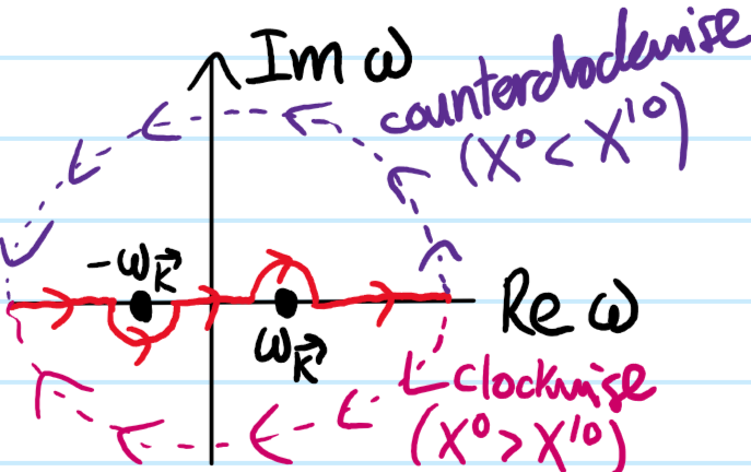
A priori, the integral is over all four-vectors \(|K\rangle\) in Minkowski spacetime which runs into trouble at the on-shell poles \(\langle K|K\rangle=k_c^2\). Thus, to be more precise, one can first write \(d^4|K\rangle=d^3\textbf kd\omega/c\) and also emphasize this by replacing \(\langle K|K\rangle-k_c^2=(\omega+\omega_{\textbf k})(\omega-\omega_{\textbf k})/c^2\), rather than integrating over the real axis \(\omega\in\textbf R\), the idea is to complexify it \(\omega\in\textbf C\) so that it hops around the on-shell poles at \(\omega=\pm\omega_{\textbf k}\) in a very specific way that enforces the time-ordering property from earlier:
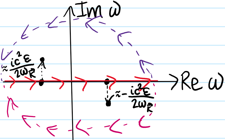
where the choice of which semicircular contour to close with is motivated by considering the time-ordering of \(X,X’\) and using Jordan’s lemma. Picking the appropriate residue in each case, one can thus verify this contour integral representation of the Feynman propagator, and indeed it is often also equivalently written without any complexification \(\omega\in\textbf R\) but instead introducing an \(i\varepsilon\)-prescription (with \(\varepsilon>0\) but infinitesimal in suitable units) to shift the poles slightly off the \(\Re\)-axis such that the pole originally at \(\omega=-\omega_{\textbf k}\) shifts slightly above the \(\Re\)-axis and vice versa for the pole at \(\omega=\omega_{\textbf k}\) to maintain the same topology as above:
(think of this as more of just a formality/notation to express a topological statement)
One last interpretation of the Feynman propagator \(\Delta_F(X-X’)\) is that, being suggestively written as a function of the argument \(X-X’\), it is essentially (irrespective of the choice of contour) a Green’s function for the Klein-Gordon operator on Minkowski spacetime:
where note that \(\partial_{\mu}=\frac{\partial}{\partial X^{\mu}}\neq\frac{\partial}{\partial X’^{\mu}}\). This means that if one wished to solve an inhomogeneous Klein-Gordon equation with some forcing field \(f(X)\), one could just convolve \(f(X)\) with the Feynman propagator \(\Delta_F(X-X’)\) as a kernel (boundary conditions tied to a choice of contour for the Green’s function? Retarded vs. advanced Green’s functions…).
Consider an arbitrary worldline \(\{(t,\textbf x)\}\) of a classical system of particles in configuration spacetime. In general, this worldline need not correspond to any physical/on-shelltrajectory; it can be as wildly off-shell as one likes, the only caveat being that time travel is forbidden (i.e. it must be possible to parameterize the worldline as \(\textbf x(t)\)).
Now take this worldline \(\{(t,\textbf x)\}\) and gently perturb each point on it \((t_0,\textbf x_0)\mapsto (t_0+\delta t(t_0,\textbf x_0),\textbf x_0+\delta\textbf x(t_0,\textbf x_0))\) by some infinitesimal translation to obtain a slightly shifted worldline. Given any generic off-shell function \(L(t,\textbf x,\dot{\textbf x})\) on configuration spacetime, if the function had value \(L(t_0,\textbf x_0,\dot{\textbf x}_0)\) at some point \((t_0,\textbf x_0)\in\{(t,\textbf x)\}\) on the worldline prior to the perturbation, then after the perturbation the value of the function at the corresponding displaced point \((t_0+\delta t(t_0,\textbf x_0),\textbf x_0+\delta\textbf x(t_0,\textbf x_0))\) on the perturbed worldline would be:
Henceforth dropping the cumbersome arguments (but keeping in mind the equation holds at any arbitrary point \((t_0,\textbf x_0)\in\{(t,\textbf x)\}\) on the unperturbed worldline), one thus has:
where \(\textbf p:=\frac{\partial L}{\partial\dot{\textbf x}}\). So far this has just been math. At this point, one has to introduce \(2\) key pieces of physics:
The function \(L(t,\textbf x,\dot{\textbf x})\) is not just some random function, but a special function called the Lagrangian, defined by \(L(t,\textbf x,\dot{\textbf x}):=T(\dot{\textbf x})-V(t,\textbf x)\).
Among the uncountably infinite ocean of worldlines \(\{(t,\textbf x)\}\) that one could weave through configuration spacetime, the tiny subset of these worldlines that are physical/on-shell are those which satisfy the stationary action principle. This means that for any pair of points \((t_1,\textbf x^*(t_1)),(t_2,\textbf x^*(t_2))\) on such an on-shell worldline \(\textbf x^*(t)\), the action functional
is stationary on \(\textbf x^*(t)\) (i.e. \(\delta S[\textbf x^*(t)]=0\)) subject to the constraints that:
The initial and final times \(t_1,t_2\) are fixed \(\delta t(t_1,\textbf x^*(t_1))=\delta t(t_2,\textbf x^*(t_2))=0\)
The initial and final configurations \(\textbf x^*(t_1),\textbf x^*(t_2)\) are also fixed \(\delta\textbf x(t_1,\textbf x^*(t_1))=\delta\textbf x(t_2,\textbf x^*(t_2))=\textbf 0\).
This yields the on-shellEuler-Lagrange equations of motion:
On the other hand, if one now relaxes the above boundary conditions (which were needed only for formulating the stationary action principle) and instead consider an arbitrary infinitesimal perturbation \((t_0,\textbf x^*(t_0))\mapsto (t_0+\delta t(t_0,\textbf x^*(t_0)),\textbf x^*(t_0)+\delta\textbf x(t_0,\textbf x^*(t_0)))\) of an on-shell trajectory \(\textbf x^*(t)\) (to emphasize again, the boundaries are now free to move!), then the on-shell action \(S^*=S[\textbf x^*(t)]\) changes by the infinitesimal virial:
Consider a free particle \(L=\frac{1}{2}m|\dot{\textbf x}|^2\). The Euler-Lagrange equations assert that such a particle moves at constant velocity \(\dot{\textbf x}=\text{const}\). Thus, all straight lines in configuration spacetime are on-shell worldlines because they make the action stationary.
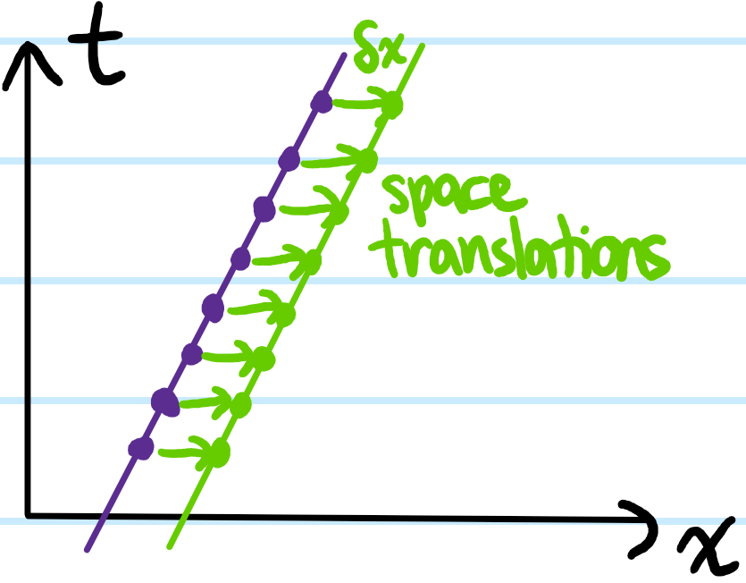
Therefore, if one starts with any such (on-shell) straight worldline \(\textbf x^*(t)\) and performs a simple space translation \(\delta\textbf x\) without any time translation \(\delta t=0\) (purple to green curve), then on the one hand the action is unchanged \(\delta S^*=0\) because the new straight worldline is still on-shell (or mathematically, \(S=\frac{m}{2}\int_{t_1}^{t_2}dt|\dot{\textbf x}(t)|^2\) but the “slope” \(|\dot{\textbf x}|\) didn’t change) but on the other hand general calculus considerations dictate it changes by \(\delta S^*=[\textbf p\cdot\delta\textbf x]^{t_2}_{t_1}\) where \(\textbf p=m\dot{\textbf x}\). One is thus forced to conclude that the quantity \(\textbf p\cdot\delta\textbf x\) (and thus \(\textbf p\) itself because \(\delta\textbf x(t_1,\textbf x(t_1))=\delta\textbf x(t_2,\textbf x(t_2))\) is a uniform space translation) is conserved (since \(t_1\leq t_2\) are arbitrary times). If one likes, this is the integral form of the conservation of momentum. The differential form \(\dot{\textbf p}=\textbf 0\) is just the on-shell Euler-Lagrange equation.
Conservation of Energy for Time-Independent Systems
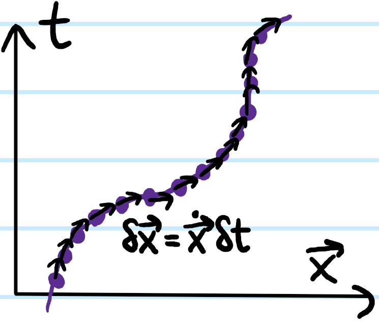
If one perturbs all the points along the curve such that the time and space perturbations are linked by the velocity \(\delta\textbf x=\dot{\textbf x}\delta t\), then this is a symmetry of the system since the on-shell action changes by a boundary term:
from which one obtains the conserved quantity \(H:=\textbf p\cdot\dot{\textbf x}-L\). In differential form, one can check the general on-shell identity \(\dot H=-\frac{\partial L}{\partial t}\) so when \(\frac{\partial L}{\partial t}=0\) one obtains \(H\) as the conserved energy (called the Beltrami identity in the more general setting of the calculus of variations). Strictly speaking \(H\) is not to be confused with the Hamiltonian which is a function of \(\textbf x\) and \(\textbf p\) via a \(\dot{\textbf x}\mapsto\textbf p\) Legendre transform of the Lagrangian \(L\).
Conservation of Angular Momentum
Finally, if the infinitesimal angular translation \(\delta\textbf x:=\delta\boldsymbol{\phi}\times\textbf x\) is a symmetry of the system, then the quantity:
is conserved, where the orbital angular momentum \(\textbf L:=\textbf x\times\textbf p\).
General Remarks on Noether’s Theorem
More generally, anything you can do to some on-shell worldline that keeps it on-shell such that the on-shell action \(\delta S^*\) changes by at most some boundary term (equivalently the Lagrangian \(L\) changes by a total time derivative) is called a symmetry of the system, and this state of affairs can always be rearranged to yield a conservation law. This is Noether’s theorem.
Thus, to recap, Noether’s theorem arises from the fact that the action \(S\) is a time integral \(\int dt\) and that when working on-shell, the variation \(\delta S^*\) in the on-shell action is zero everywhere along the main body of the worldline \(\textbf x^*(t)\) (thanks to the stationary action principle) and so is only sensitive to the “edge effects” associated with changes in the initial and final configurations. But if the perturbation is a symmetry of the system, then one can always reframe this as saying that some quantity is conserved. Implicit in the whole discussion is that these symmetries need to be elements of some continuous Lie group otherwise it wouldn’t be possible to speak of implementing them infinitesimally.
Also, for any kind of purely spatial perturbation \(\delta\textbf x(t)\) so that \(\delta t=0\), it doesn’t even matter if \(\partial L/\partial t\neq 0\)…
Problem: What is the defining property of the (Cauchy) stress tensor (field) \(\sigma(\textbf x,t)\) of a material.
Solution: The idea is that if one wants to find the stress vector (also called traction) \(\boldsymbol{\sigma}\) acting on a plane with unit normal \(\hat{\textbf n}\) in the material at location \(\textbf x\) and time \(t\), then this is obtained by acting with the stress tensor:
\[\boldsymbol{\sigma}=\sigma\hat{\textbf n}\]
Or in components:
\[\sigma_i=\sigma_{ij}n_j\]
Problem: What do the diagonal stresses \(\sigma_{11},\sigma_{22},\sigma_{33}\) represent physically? What about the off-diagonal stresses \(\sigma_{12},\sigma_{23},\sigma_{13}\), etc.
Solution: The diagonal stresses represent normal stresses. The off-diagonal stresses represent shear stresses.
Problem: Under what conditions is the stress tensor \(\sigma^T=\sigma\) symmetric? What does this imply the existence of?
Solution: Provided the net couple/torque vanishes \(\boldsymbol{\tau}=\textbf 0\) (intuitively, the normal stresses do not supply any torque, it is the off-diagonal shear stresses that need to match to ensure this rotational equilibrium).
The immediate corollary of this is that, as usual, \(\sigma\) will have \(3\) orthogonal eigenspaces (called principal directions spanned by \(\hat{\textbf n}\), whose orthogonal complements \(\text{span}^{\perp}(\hat{\textbf n})\) are called the principal planes) each associated to a real eigenvalue (called a principal stress). Physically, the stress vector \(\boldsymbol{\sigma}\) acts perpendicularly to such principal planes along the principal directions, so it is a pure normal stress since when diagonalized the off-diagonal shear stresses vanish.
Problem: If \(\sigma_{1,2,3}\) is a principal stress of the stress tensor \(\sigma\), explain why:
Solution: This is a bit trivial in that it’s just the general form of the characteristic equation for any \(3\times 3\) matrix. Equally trivial is the fact that coefficients are coordinate-free (and sometimes called stress invariants in this context). In terms of the principal stresses \(\sigma_1,\sigma_2,\sigma_3\) at a given point in spacetime (not to be confused with the components of the stress vector), of course one has:
Problem: Suppose one were interested in just the normal stress in the direction \(\hat{\textbf n}\) at some point even though the stress vector \(\boldsymbol{\sigma}\) was not parallel with \(\hat{\textbf n}\) (i.e. not a principal direction!). How can one nevertheless extract this information?
Solution: Do the obvious thing \(\hat{\textbf n}\cdot\boldsymbol{\sigma}=\hat{\textbf n}^T\sigma\hat{\textbf n}=\sigma_{ij}n_in_j\).
Problem: (Mohr’s circle, (equivalent) von Mises stress, yield criteria, cool Lagrange multiplier optimization problem for max/min shear stresses in Tresca’s criterion)
Solution:
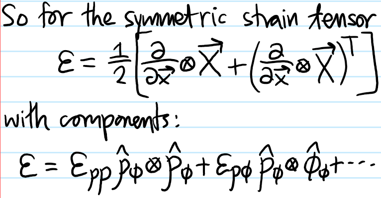
Problem: What is the definition of the strain tensor \(\varepsilon\)?
Solution: It is the symmetric part of the Jacobian of the displacement field \(\textbf X(\textbf x,t)\), i.e.
and therefore is by construction symmetric \(\varepsilon^T=\varepsilon\).
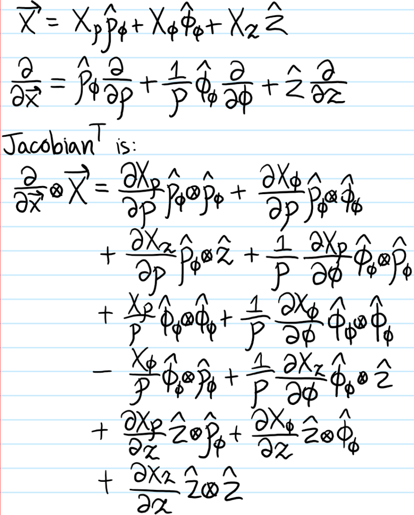
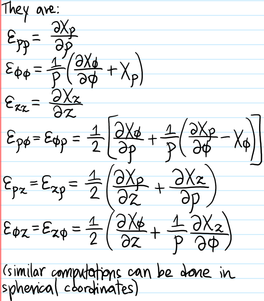
Problem: Find the components of the strain tensor \(\varepsilon\) in cylindrical coordinates.
Solution:
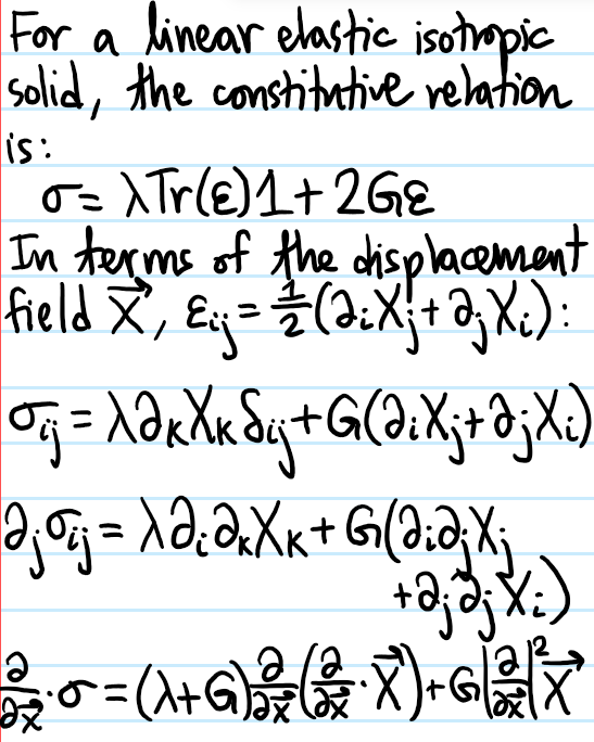
Problem: Describe the grown-up version of Hooke’s constitutive law relating \(\varepsilon\) to \(\sigma\).
Solution: At its essence, Hooke’s law postulates there exists a linear and elastic (i.e. in thermodynamics language, reversible, i.e. no hysteresis) relationship between them, given by a rank-\(4\) tensor field \(C\) (called the elasticity/stiffness tensor):
\[\sigma=C\varepsilon\]
Or, more transparently in Cartesian components:
\[\sigma_{ij}=C_{ijk\ell}\varepsilon_{k\ell}\]
Although a general rank-\(4\) tensor in \(3\)D has \(3^4=81\) degrees of freedom, the symmetries \(\sigma_{ij}=\sigma_{ji}\) and \(\varepsilon_{ij}=\varepsilon_{ji}\) means that \(C_{ijk\ell}=C_{jik\ell}\) and \(C_{ijk\ell}=C_{ij\ell k}\) so the first \(2\) indices \(\{i,j\}\) should be viewed as a multiset rather than an ordered pair, and similarly for the last \(2\) indices \(\{k,\ell\}\). By inspection, there are \(3+2-1\choose{2}\)\(=6\) such multisets, for a total of \(6^2=36\) degrees of freedom. However, the existence of a scalar elastic strain energy density \(\frac{1}{2}C_{ijk\ell}\varepsilon_{ij}\varepsilon_{k\ell}\) means that \(C_{ijk\ell}=C_{k\ell ij}\), so a \(6\times 6\) symmetric matrix has \(\frac{6\times 7}{2}=21\) independent degrees of freedom.
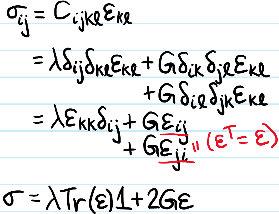
Problem: Imposing further the assumption that \(C\) is an isotropic tensor, explain why \(21\) degrees of freedom are reduced to just \(2\):
Solution: Start with Hooke’s law for a linear-elastic material, and then inject isotropy into \(C\):
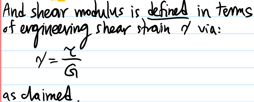
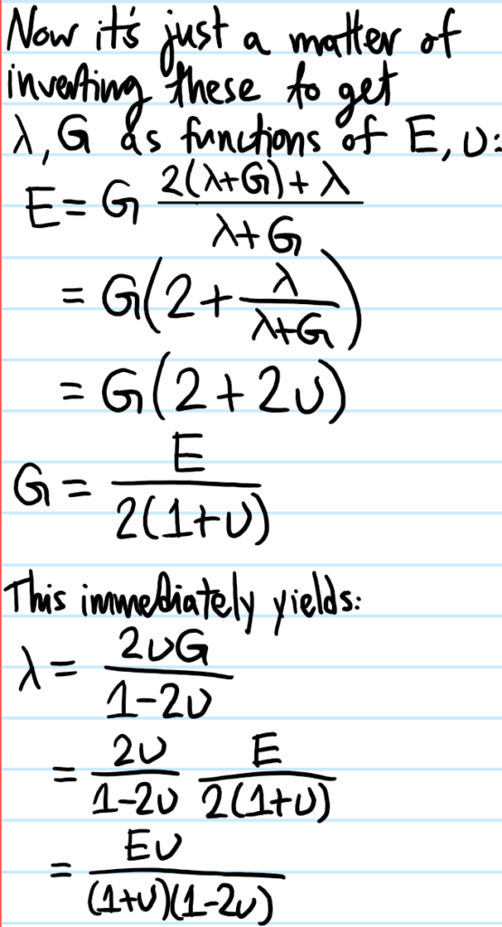
Problem: It is important to emphasize the number “\(2\)” in the statement “there are \(2\) Lame parameters \(\lambda, G\)”. Just as in the thermodynamics of a gas the state of the system is completely specified by \((p,V)\), similarly here any linear-elastic isotropic material’s behavior is completely specified by \(2\) independent moduli, such as \((\lambda, G)\). However, there are also other pairs of moduli available, such as \((E,\nu)\) (Young’s modulus with Poisson’s ratio) or \((B, G)\) (bulk modulus and shear modulus).
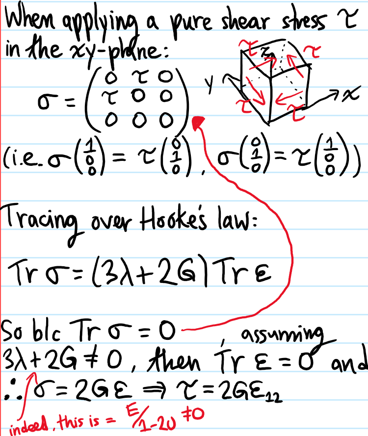
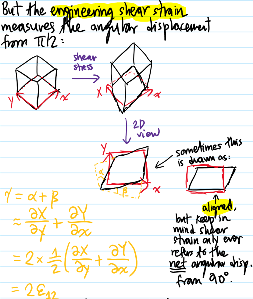
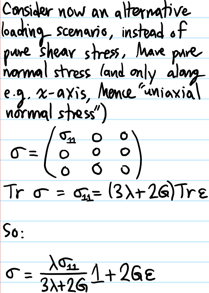
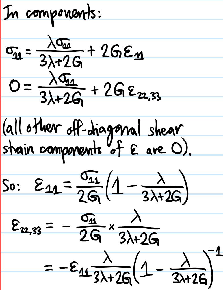
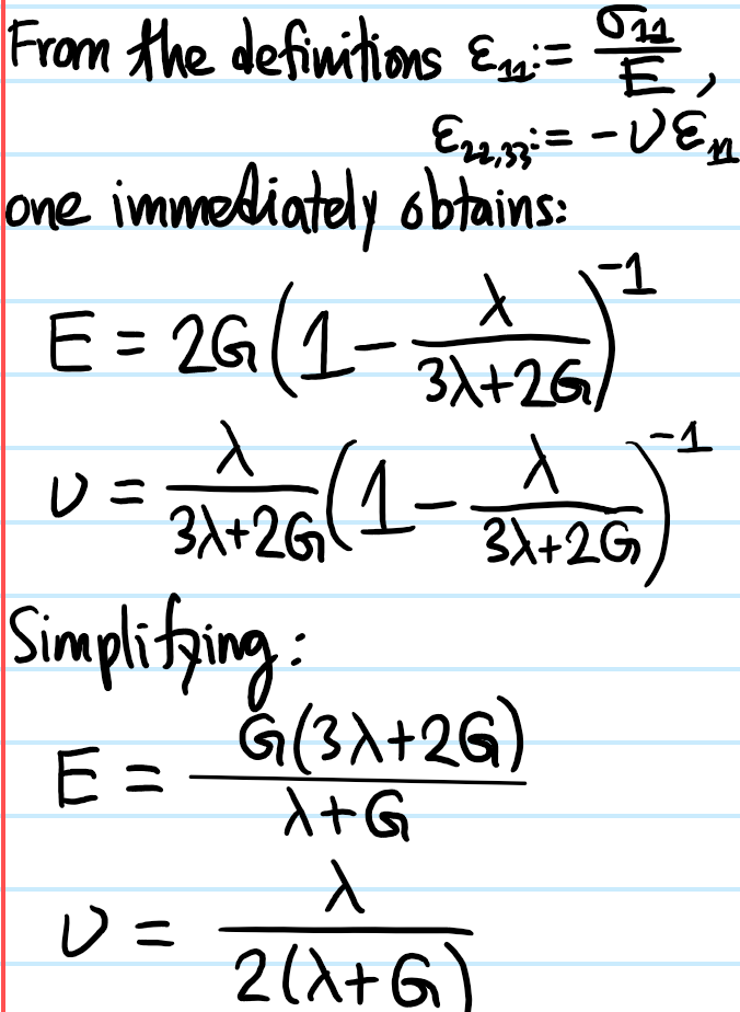
First, explain why the \(G\) here really deserves to be called “shear modulus”. Similarly, by considering other loading scenarios, show that the relevant “Legendre transformations” between the moduli are:
\[\lambda=\frac{E\nu}{(1+\nu)(1-2\nu)}\]
\[G=\frac{E}{2(1+\nu)}\]
\[B=\frac{E}{3(1-2\nu)}\]
Solution:
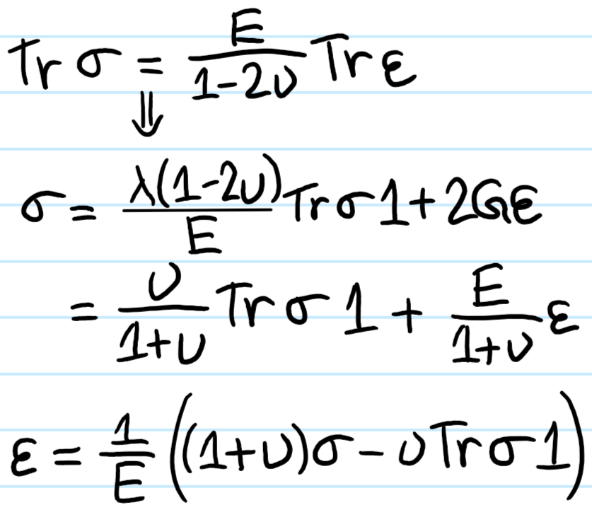
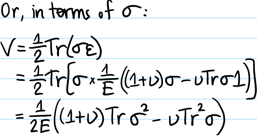
Problem: Hooke’s law for linear-elastic materials as it’s currently written:
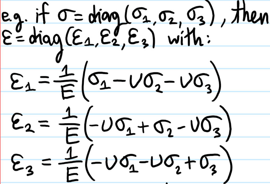
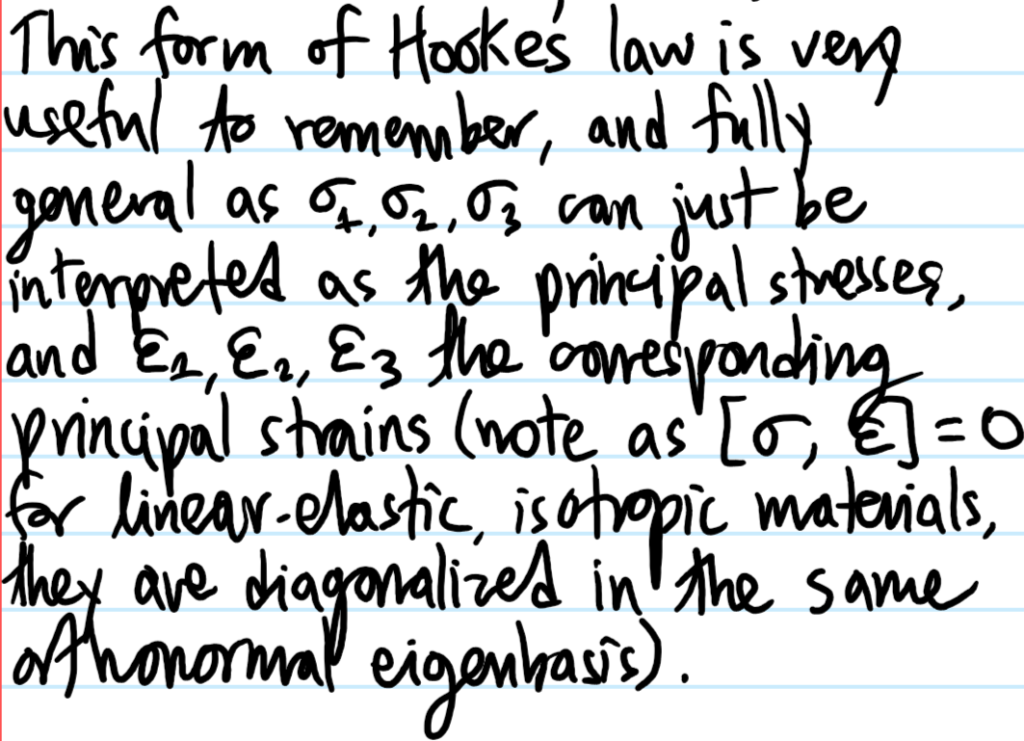
conflates cause-and-effect since \(\sigma\) is what causes \(\varepsilon\). Show how to isolate for \(\varepsilon\) in terms of \(\sigma\), and write the resultant Hooke’s law in the principal frame.
Solution:
Problem: Looking at the expression for the bulk modulus \(B\) in terms of \(E\) and \(\nu\):
\[B=\frac{E}{3(1-2\nu)}\]
Explain why this constrains \(\nu\leq 1/2\). What does it mean for a material (e.g. rubber) to have \(\nu=1/2\)?
Solution:Stability requires that \(B\geq 0\) (otherwise one would get a positive feedback loop between \(p,V\)), so this implies \(\nu\leq 1/2\). Materials with \(\nu=1/2\) are volume-preserving; stretching in \(z\) will causes a contraction in \(\rho\) such that \(z\rho^2=\text{const}\). Of course this means the bulk modulus is \(B=\infty\).
Problem: How is this grown-up version of Hooke’s law related to the childish version \(F=-kx\)?
Solution: For a spring of material with Young’s modulus \(E\), wire of cross-section \(A\), and length \(L\), the spring constant is:
\[k=\frac{EA}{L}\]
this should be compared with a similar formula for capacitance of a parallel-plate capacitor:
\[C=\frac{\varepsilon A}{d}\]
or inductance of a long solenoid:
\[L=\frac{\mu N^2A}{\ell}\]
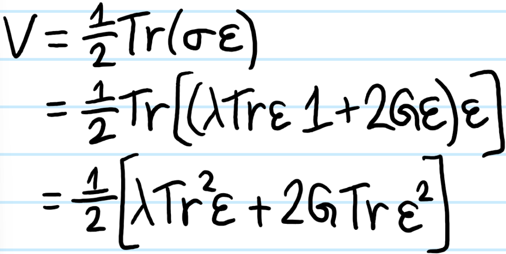
Problem: Explain why, as claimed earlier, for any (possibly anisotropic) linear elastic material, the strain energy density \(V\) is given by:
And show how this result specializes to the case of an isotropic linear elastic material.
Solution: Basically just the usual argument of doing some work on a unit cell and equating that with the stored energy; the factor of \(1/2\) is the canonical “area-of-a-triangle” factor that arises due to the linearity of the stress-strain “curve”.
Including the assumption of isotropy:
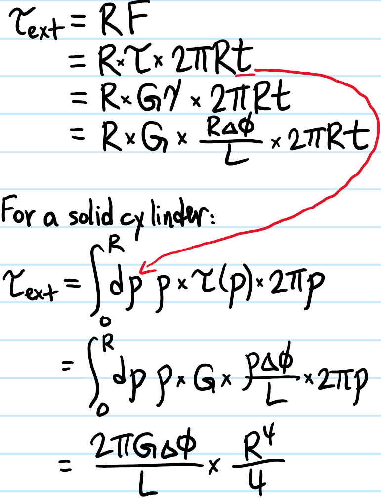
Problem: Consider twisting a hollow cylinder of radius \(R\), length \(L\), and thickness \(t\ll R\) through a small angle \(\Delta\phi\). Show that the external couple \(\tau_{\text{ext}}\) required to maintain this is:
(optional: calculate the elastic strain energy stored in the cylinders in both cases).
Solution:
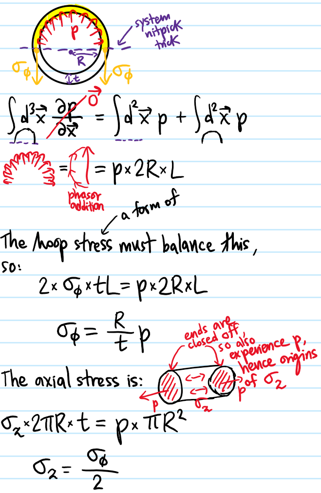
Problem: Consider a uniformly pressurized hollow, capped cylinder of pressure \(p\), radius \(R\), thickness \(t\) and length \(L\). Show that the hoop stress \(\sigma_{\phi}\) and axial stress \(\sigma_z\) are related by a factor of \(2\):
\[\sigma_{\phi}=2\sigma_{z}=\frac{R}{t}p\]
(WHAT ABOUT RADIAL STRESSES \(\sigma_{\rho}\)?)
Solution:
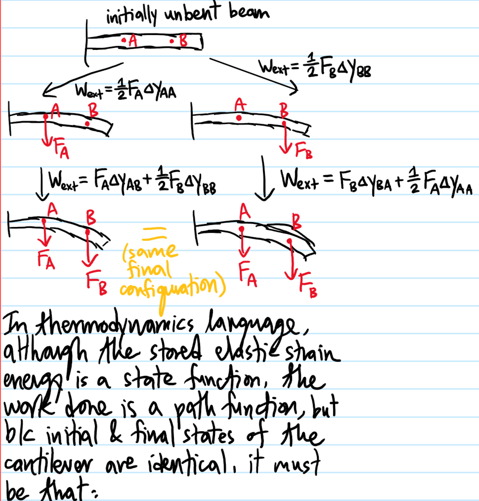
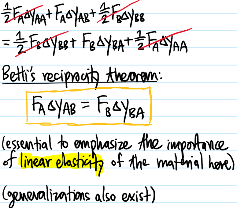
Problem: Demonstrate Betti’s reciprocity theorem for a linear elastic isotropic cantilever beam.
Solution:
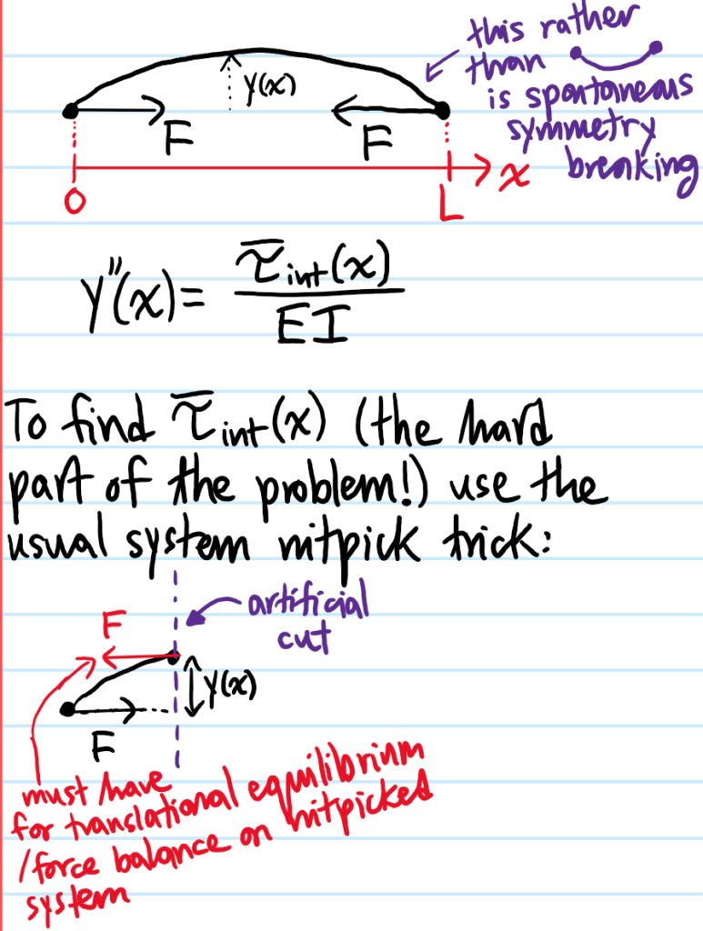
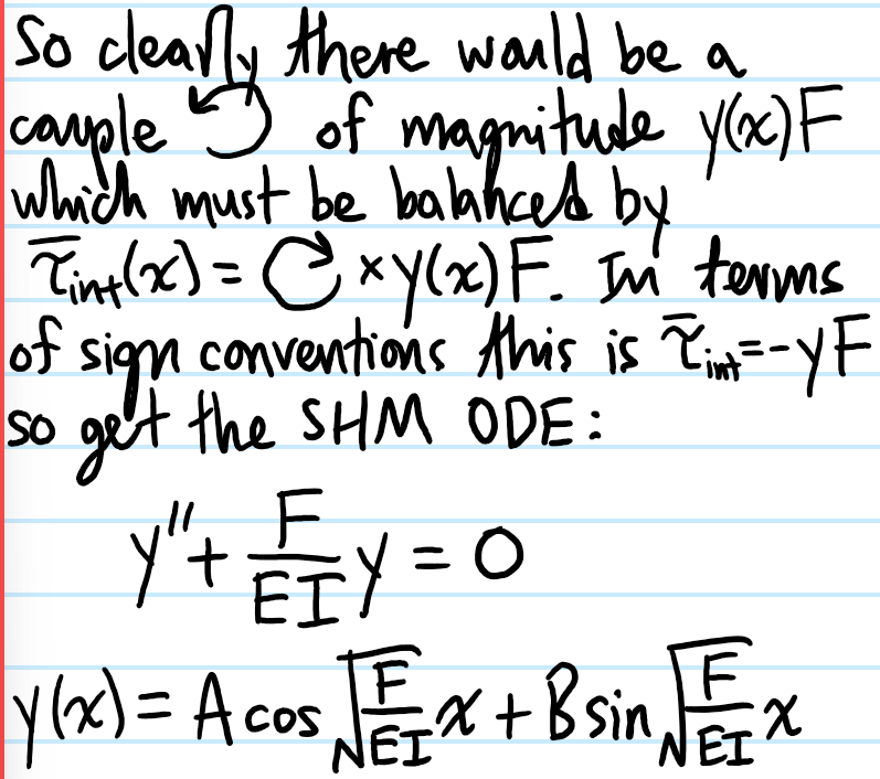
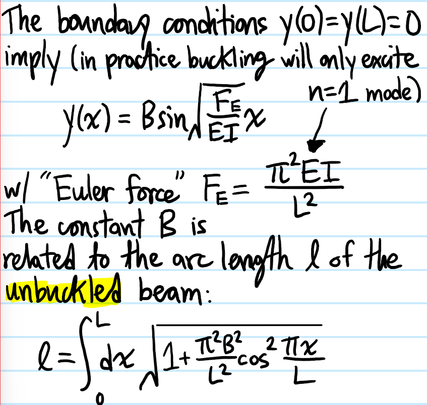
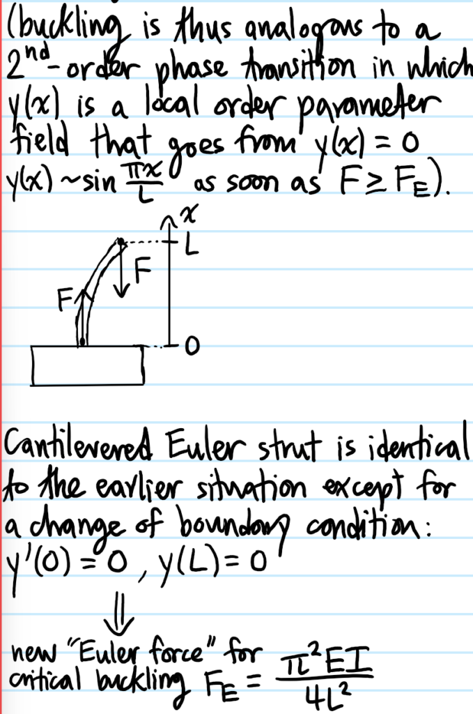
Problem: Show that if one takes a beam with Young’s modulus \(E\), moment of area \(I\), and you start to compress it axially, once the force \(F\) applied exceeds a certain critical force (the “Euler force”), the beam will spontaneously break symmetry by buckling (this configuration is sometimes referred to as the Euler strut).
Solution:
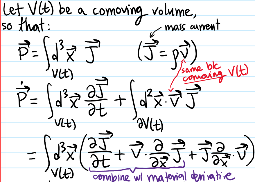
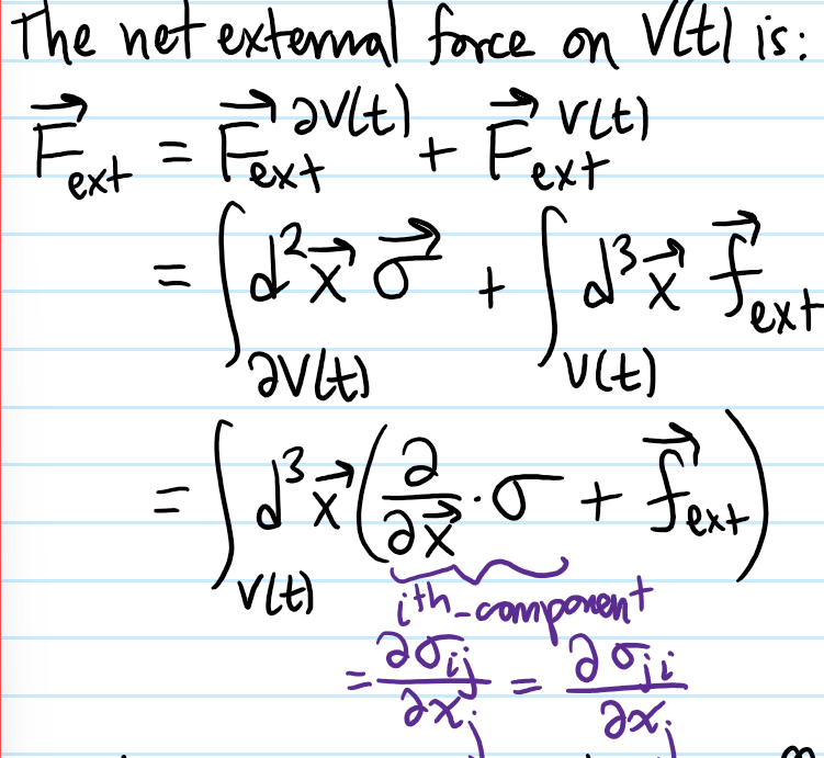
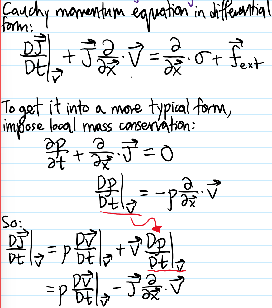
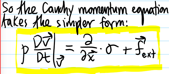
Problem: Show that Newton’s \(2^{\text{nd}}\) law in a continuum becomes the Cauchy momentum equation:
Solution: Basically just an application of the Reynold’s transport theorem to a system nitpick trick applied to a comoving volume:
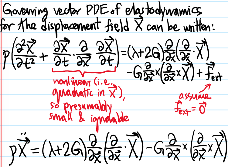
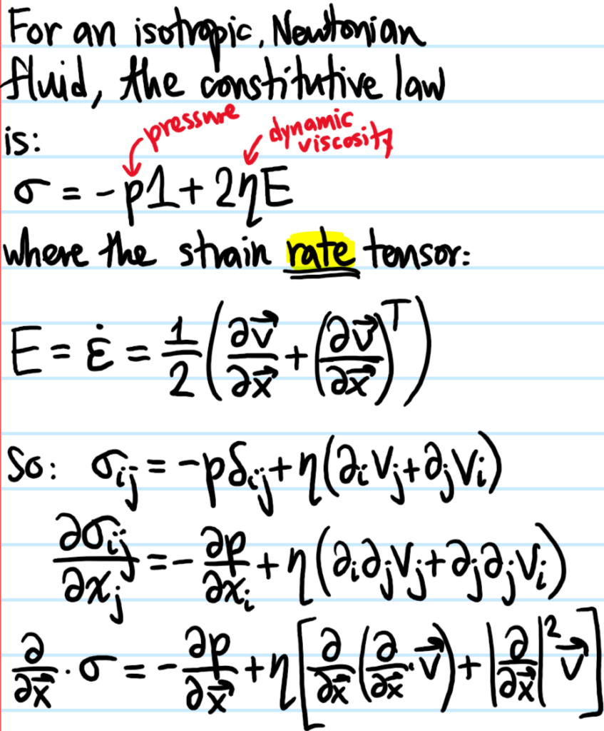
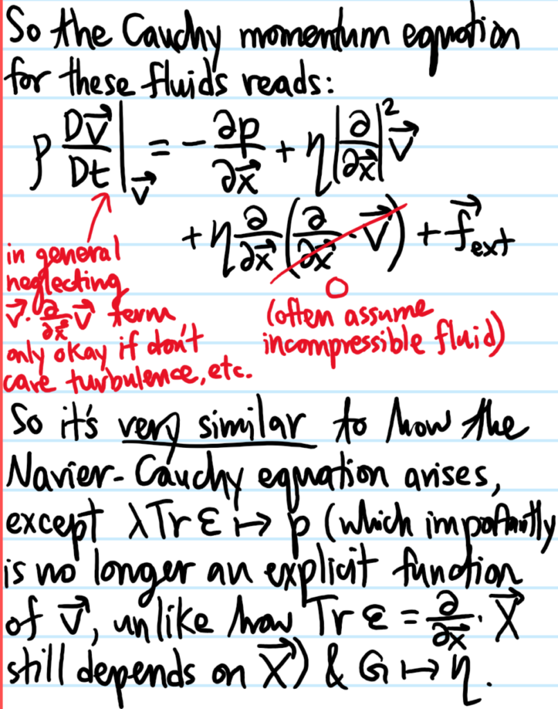
Problem: Show how, using the Cauchy momentum equation as the fundamental starting point, the equations of elastodynamics (Navier-Cauchy equations) and fluid dynamics (Navier-Stokes equations) arise from postulating similar-looking but conceptually different constitutive relations for the stress tensor \(\sigma\).
Solution:
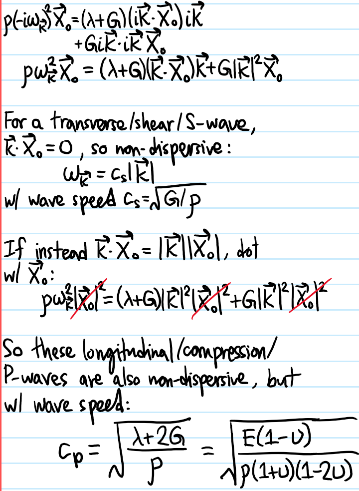
Problem: As the Navier-Cauchy equations are linear, it makes sense to consider a plane wave ansatz \(\textbf X(\textbf x,t)=\textbf X_0e^{i(\textbf k\cdot\textbf x-\omega_{\textbf k}t)}\). Hence show that there are \(2\) kinds of waves:
obtain the dispersion relation \(\omega_{\textbf k}\) for \(S\)-waves and \(P\)-waves (cf. \(s\) and \(p\) atomic orbitals or \(s\)-wave and \(p\)-wave scattering in quantum mechanics…the nomenclature is a coincidence as here \(S\) stands for “secondary” while \(P\) stands for “primary”, whereas in the quantum context \(s\) stands for “sharp” while \(p\) stands for “principal”).
Solution:
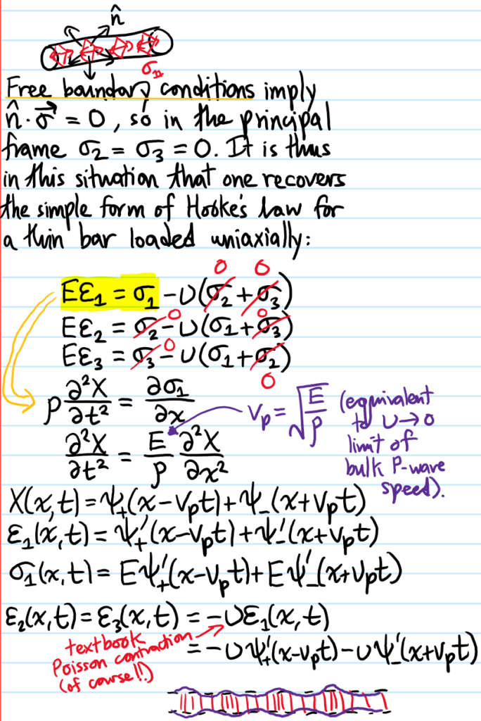
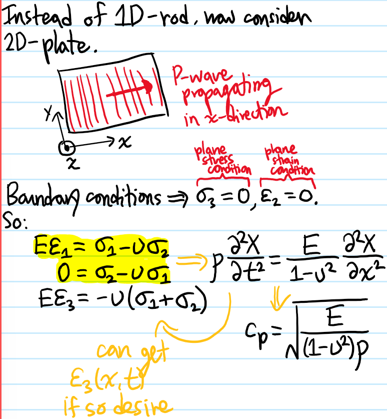
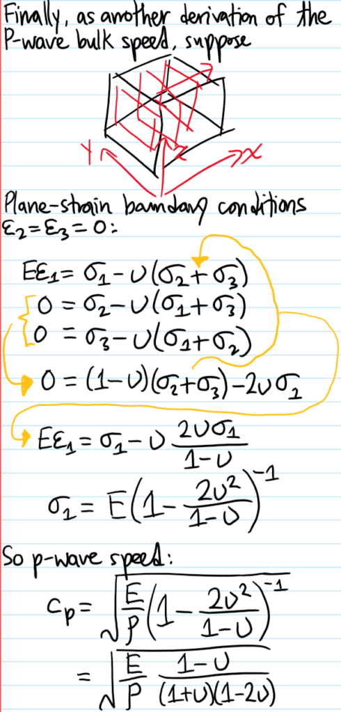
Problem: Consider a longitudinal \(P\)-wave propagating in the \(x\)-direction through:
a) A \(1\)D infinite (linear elastic isotropic) rod.
b) A \(2\)D infinite (linear elastic isotropic) plate.
c) A \(3\)D infinite (linear elastic isotropic) bulk solid.
In each case, what is the speed \(v_p\) of such \(P\)-waves?
Solution:
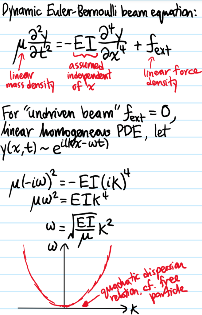
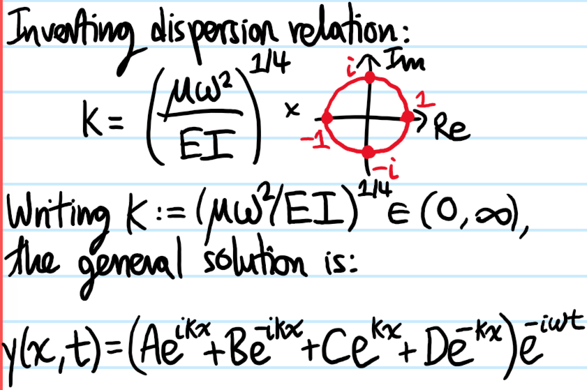
Problem: Starting from the Navier-Cauchy equations, show how to obtain the dynamic Euler-Bernoulli beam equation.
Solution:
Problem: Find the normal mode frequencies of vibration \(\omega_n\) of a cantilever beam of length \(L\).
Solution:
So the allowed values of \(kL\), although strictly given by the zeroes of the graph, quickly tend towards \(k_nL\approx (n+1/2)\pi\) (which are the vertical dashed lines). By the dispersion relation, the corresponding angular frequencies therefore quickly tend toward:
Problem: What is the sign convention for the internal couple (also called bending moment) of a beam?
Solution: Remember the mnemonic “top in tension” as this is when \(\bar{\tau}_{\text{int}}(x)>0\). For instance, for a simple cantilever beam drooping under its own weight, the top of the beam is clearly in tension everywhere, so the internal couple will be positive all the way along. Similarly, for a beam which is sagging between \(2\) supports, the top is in compression everywhere so under this sign convention the internal couple is negative everywhere along the beam.
Problem:
The advantage of this convention is that the static Euler-Bernoulli beam equation doesn’t need any pesky minus signs, assuming also the (reasonable) convention that \(y(x)>0\) is an upwards displacement:
\[y”(x)=\bar{\tau}_{\text{int}}(x)/EI\]
Geometrically, it is intuitively clear that when a beam is bent by external forces and torques, some sections will become longer (hence experiencing internaltension) while other sections will become shorter (hence experiencing internalcompression). By the intermediate value theorem, there thus exists a section which becomes neither longer nor shorter, instead possessing a bend-invariant length; this is called the neutral axis of the beam (strictly speaking, the neutral axis is not a 1D line, but a 2D surface cutting through the center of the beam so perhaps a better name would have been neutral surface). The neutral axis of the beam therefore experiences neither internal tension nor internal compression, and so is defined by experiencing zero internal stress \(\sigma_{\text{int}}=0\). The idea is to then understand how the internal stress field \(\sigma_{\text{int}}(y)\) varies as a function of the distance \(y\) above (or below) the neutral axis (where we’ve just established it’s zero). Intuitively, this should depend not only on \(y\), but also on the stiffness of the beam material (this is why it’s harder to bend stiffer beams!). Since the internal tensions and internal compressions are essentially uniaxial stresses along the beam, one should invoke Hooke’s law:
$$\sigma_{\text{int}}(y)=E\varepsilon(y)$$
where the engineering strain \(\varepsilon(y)\) at a distance \(y\) from the neutral axis may be approximated as \(\varepsilon(y)=\kappa y\) where \(\kappa\) is the local curvature of the beam (and the key reason for introducing it is that it is independent of \(y\), being only a function of position \(x\) along the neutral axis). Thus, the key finding here is that the internal stress field varies linearly about the neutral axis:
$$\sigma_{\text{int}}(y)=\kappa Ey$$
Throughout this, the analysis has been for some fixed \(x\), and looking at the variation in \(y\). To globalize this from \(y\to x\), one could stick with \(\sigma_{\text{int}}(x,y)=\kappa(x)Ey\) but this would still be mucking up \(x\) with \(y\). So in order to get rid of \(y\) and be able to just worry about \(x\), it is necessary to find some property that characterizes each cross section of the beam. Staring at the picture of the internal stress field, it is clear that one useful metric is provided by the internal torque \(\bar{\tau}_{\text{int}}(x)\) about the neutral axis (also called the internal bending moment by engineers), which by definition is:
$$\bar{\tau}_{\text{int}}(x)=\iint_{\text{cross section at }x}y\sigma_{\text{int}}(x,y)dA$$
Introducing the second moment of area \(\bar I(x):=\iint_{\text{cross section at }x}y^2dA\) about the neutral axis, this leads to the result:
which washes out all \(y\)-dependence as desired. The product \(E\bar I\) is called the flexural rigidity of the beam. Letting \(\delta(x)\) denote the profile of the bent beam, one has the approximation \(\kappa(x)\approx d^2\delta/dx^2\), so (suppressing the \(x\)-dependence):
Finally, although this form is generally sufficient (thanks to the “system nitpick trick”), it is also possible to express the internal torque \(\bar{\tau}_{\text{int}}\) about the neutral axis directly in terms of the (perhaps more intuitive) linear external transverse force density \(f_{\text{ext}}^{\perp}(x)\) along the beam. Specifically, because the beam is static, translational equilibrium in the vertical direction gives \(f_{\text{ext}}^{\perp}(x)=\frac{dF_{\gamma}}{dx}\) where \(F_{\gamma}(x)\) is the vertical shear force at position \(x\) and rotational equilibrium gives \(F_{\gamma}(x)=\frac{d\bar{\tau}_{\text{int}}}{dx}\). Altogether, this yields a 4th-order ODE which is traditionally called the static Euler-Bernoulli beam equation:
Evidently, a more descriptive name for the static Euler-Bernoulli beam equation would be the static small deflection beam equation since the most important assumption underlying it is that the deflection \(\delta(x)\) of the beam is small everywhere.
Example: Within the Euler-Bernoulli small deflection regime, what is the shape of a homogeneous cantilever beam of density \(\rho\), Young’s modulus \(E\), and length \(L\) with an \(a\times a\) square cross section in the presence of Earth’s surface gravitational field \(g\)? One option is to insert \(f_{\text{ext}}^{\perp}=\rho ga^2\) and integrate the static Euler-Bernoulli beam equation from \(0\) to \(L\) with respect to \(x\). Because the internal shear force \(F_{\gamma}(0)=\rho ga^2L\) at the fixed end must balance the weight of the cantilever, this gives a boundary condition to fix the first integration constant. Integrating again, and now using the boundary condition \(\bar{\tau}_{\text{int}}(0)=\rho ga^2L^2/2\), one gets a second boundary condition. Then integrating twice more and using the cantilever boundary conditions \(\delta(0)=d\delta/dx(0)=0\) yields the deflected beam profile as a quartic polynomial in \(x\):
with maximum deflection \(\delta(L)=\frac{3\rho gL^4}{2a^2E}\), so if one wished to minimize this, then a suitable merit index for materials selection would be \(E/\rho\).
For Mode I plane stress crack loading, an external stress \(\boldsymbol{sigma}_{\text{ext}}\) is applied which induces a uniform internal stress field \(\sigma\) in the material. A crack of “semi-major axis” \(a\) will grow/propagate iff \(a>a^*=\frac{EV’_I}{\pi\sigma^2_{\text{ext}}}\). For brittle materials, \(\mathcal G^*=2\gamma\) (I don’t like the notation, but it’s so common I’ll just use it; maybe think Gibbs free energy is also a sort of “energy released”?), but for ductile materials the potential energetic penalty \(\mathcal G^*\) is generally far greater due the formation of a plastic zone about the crack tip \(\sigma_{\text{int}}=\sigma^*\) which requires external work \(W_{\text{ext}}=\frac{(\sigma^*)^2}{2E}\) to form (since it’s plastic deformation just like doing any other kind of deformation! Or think about the dislocations?). This blunts the crack tip curvature. The punchline is that ductile = tough! Also, fracture toughness \(\mathcal K^*:=\sqrt{E\mathcal G^*}\) (idk why the K notation). So basically, shit breaks when you drop it on the floor for instance because at the moment of collision the high stress \(\sigma_{\text{ext}}\) lowered the critical crack size \(a^*\propto\frac{1}{\sigma_{\text{ext}}^2}\) so much that the natural cracks \(a\) always present as defects in the material (dislocations are the other key kind of defect) exceeded \(a^*\), and therefore by the Griffith criterion it was energetically favorable for them to grow/propagate, leading to fracture! (although depends on brittle vs. ductile again).
A material is said to be viscoelastic iff it exhibits a duality between behaving as a Newtonian fluid (with some dynamic viscosity \(\eta\), hence the visco part of “viscoelastic”) and a linear elastic solid (with some Young’s modulus \(E\), hence the elastic part of “viscoelastic”) (cf. with wave-particle duality in quantum mechanics). There are various ways to make this duality precise, for instance the simplest is to model a viscoelastic material via the Maxwell model, namely a viscous damper (also called a dashpot) of dynamic viscosity \(\eta\) in series with a linear elastic spring of Young’s modulus \(E\). By Newton’s second law (analog of Kirchoff’s laws for electric circuits), this gives rise to a constitutive relation between the external stress \(\sigma_{\text{ext}}\) applied to the viscoelastic Maxwell material and its total elastic strain \(\varepsilon\) as:
This is not really a differential equation, it’s just saying if you know a priori what the applied external stress \(\sigma_{\text{ext}}=\sigma_{\text{ext}}(t)\) is, then by time integration one can recover the corresponding elastic strain \(\varepsilon(t)\) experienced by the sample. This viscoelastic duality is directly responsible for loading-unloading hysteresis of materials (i.e. the damper dissipates heat energy, corresponding to the enclosed area on a hysteresis loop).