
Problem: In numerical computation, what are the \(2\) main kinds of rounding error?
Solution: Overflow error (\(N\approx\infty\)) but perhaps even more dangerous is underflow error (\(\varepsilon\approx 0\)) which are in some sense inverses of each other:
\[0=\frac{1}{\infty}\]
Problem: Explain how rounding errors can affect evaluation of the softmax activation function and strategies to address it.
Solution: Given a vector \(\mathbf x\in\mathbf R^n\), the corresponding softmax probability \(\ell^1\)-unit vector is \(e^{\mathbf x}/|e^{\mathbf x}|_1\in S^{n-1}\). If one of the components of \(\mathbf x\) is very negative, then the corresponding component of \(e^{\mathbf x}\) can underflow, whereas if it is instead very positive, then overflow becomes a possibility.
To address these numerical stability issues, the trick is to notice that softmax is invariant under “diagonal” translations along \(\mathbf 1\in\mathbf R^n\), i.e. \(\mathbf x\mapsto\mathbf x-\lambda\mathbf 1\) leads to \(e^{\mathbf x-\lambda\mathbf 1}=e^{\mathbf x}\odot e^{-\lambda\mathbf 1}=e^{-\lambda}e^{\mathbf x}\) and hence the \(\ell^1\)-norm \(|e^{\mathbf x-\lambda\mathbf 1}|_1=e^{-\lambda}|e^{\mathbf x}|_1\) is also merely scaled by the same factor \(e^{-\lambda}\). Choosing \(\lambda:=\text{max}(\mathbf x)\) to be maximum component of \(\mathbf x\) (which coincides with the \(\ell^{\infty}\) norm if \(\mathbf x\geq 0\) is positive semi-definite) would eliminate any overflow error that may have been present in evaluating the numerator \(e^{\mathbf x}\) by instead evaluating \(e^{\mathbf x-\text{max}(\mathbf x)\mathbf 1}\). For the same reason, the shifted denominator \(|e^{\mathbf x-\text{max}(\mathbf x)\mathbf 1}|_1\) is also immune to overflow error. Furthermore, the denominator is also resistant to underflow error because at least one term in the series for \(|e^{\mathbf x-\lambda\mathbf 1}|_1=\sum_{i}e^{x_i-\lambda}\) will be \(e^0=1\gg 0\), namely term \(i=\text{argmax}(\mathbf x)\). The only possible problem is that the modified numerator could still experience an underflow error; this would be bad if subsequently one were to evaluate the information content (loss function) of a softmax outcome in which taking \(\log(0)=-\infty\) would produce a nan. For this case, one can apply a similar trick to numerically stabilize the computation of this logarithm.
Problem: Describe the numerical analysis phenomenon of catastrophic cancellation.
Solution: Subtraction \(f(x,y):=x-y\) is ill-conditioned when \(x\approx y\). This is because even if \(x\) and \(y\) have small relative errors, the relative error in their difference \(f(x,y)\) can still be substantial.
Problem: What does the condition number of a matrix \(X\) measure?
Solution: The condition number measures how numerically stable it is to invert \(X\mapsto X^{-1}\). It is given by the ratio of the largest to smallest eigenvalues of \(X\) (by absolute magnitude, assuming \(X\) is diagonalizable):
\[\frac{\text{max}|\text{spec}(X)|}{\text{min}|\text{spec}(X)|}\]
For instance, a non-invertible matrix would have \(\text{min}|\text{spec}(X)|=0\) and thus an infinite condition number, since it’s non-invertible.
Problem: Show that during gradient descent of a scalar field \(f(\mathbf x)\), if at some point \(\mathbf x\) in the optimization landscape, one has \(\frac{\partial f}{\partial\mathbf x}\cdot\frac{\partial^2 f}{\partial\mathbf x^2}\frac{\partial f}{\partial\mathbf x}>0\) (e.g. such as if the Hessian \(\frac{\partial^2 f}{\partial\mathbf x^2}\) is just generally positive-definite or the gradient \(\frac{\partial f}{\partial\mathbf x}\) is an eigenvector of the Hessian \(\frac{\partial^2 f}{\partial\mathbf x^2}\) with positive eigenvalue), then by a line search logic, the most effective local learning rate \(\alpha(\mathbf x)>0\) is given by:
\[\alpha(\mathbf x)=\frac{\left|\frac{\partial f}{\partial\mathbf x}\right|^2}{\frac{\partial f}{\partial\mathbf x}\cdot\frac{\partial^2 f}{\partial\mathbf x^2}\frac{\partial f}{\partial\mathbf x}}\]
Solution: Since gradient descent takes a step \(\mathbf x\mapsto\mathbf x-\alpha\frac{\partial f}{\partial\mathbf x}\), and the goal is to decrease the value of the function \(f\) as much as possible to get closer to the minimum, one would like to maximize:
\[f(\mathbf x)-f\left(\mathbf x-\alpha\frac{\partial f}{\partial\mathbf x}\right)\]
as a function of the learning rate \(\alpha>0\). Assuming that a quadratic approximation is valid:
\[f(\mathbf x)-f\left(\mathbf x-\alpha\frac{\partial f}{\partial\mathbf x}\right)\approx \alpha\left|\frac{\partial f}{\partial\mathbf x}\right|^2-\frac{\alpha^2}{2}\frac{\partial f}{\partial\mathbf x}\cdot\frac{\partial^2 f}{\partial\mathbf x^2}\frac{\partial f}{\partial\mathbf x}\]
which has a well-defined maximum of the \(\alpha\)-parabola provided the \(\alpha^2\) coefficient is positive.
Problem: Explain why gradient descent is behaving like this in this case? What can be done to address that?
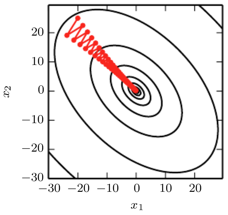
Solution: The problem is that the Hessian is ill-conditioned (in this case the condition number is \(5\) everywhere); the curvature in the \((1,1)\) direction is \(5\times\) greater than the curvature in the \((1,-1)\) direction. Gradient descent wastes time repeatedly descending “canyon walls” because it sees those as the steepest features. A \(2^{\text{nd}}\)-order optimization algorithm (e.g. Newton’s method) that uses information from the Hessian would do better.
Problem: Explain how the Karush-Kuhn-Tucker (KKT) conditions generalize the method of Lagrange multipliers.
Solution: The idea is, in addition to equality constraints like \(x+y=1\), one can also allow for inequality constraints like \(x^2+y^2\leq 1\) (indeed, an equality \(a=b\) is just \(2\) inequalities \(a\leq b\) and \(a\geq b\)). Then, constrained optimization of a scalar field \(f(\mathbf x)\) subject to a bunch of equality constraints \(g_1(\mathbf x)=g_2(\mathbf x)=…=0\) and a bunch of inequality constraints \(h_1(\mathbf x),h_2(\mathbf x),…\leq 0\) is equivalent to unconstrained optimization of the Lagrangian:
\[L(\mathbf x,\boldsymbol{\lambda}_{\mathbf g},\boldsymbol{\lambda}_{\mathbf h})=f(\mathbf x)+\boldsymbol{\lambda}_{\mathbf g}\cdot\mathbf g(\mathbf x)+\boldsymbol{\lambda}_{\mathbf h}\cdot\mathbf h(\mathbf x)\]
where \(\boldsymbol{\lambda}_{\mathbf g},\boldsymbol{\lambda}_{\mathbf h}\) are called KKT multipliers. The KKT necessary (but not sufficient!) conditions for optimality are then (ignoring technicalities about equating objects of possibly different dimensions):
- \(\frac{\partial L}{\partial\mathbf x}\mathbf 0\) (stationary)
- \(\mathbf g(\mathbf x)=\mathbf 0\geq \mathbf h(\mathbf x)\) (primal feasibility)
- \(\boldsymbol{\lambda}_{\mathbf h}\geq 0\) (if the inequalities were instead written as \(\mathbf h(\mathbf x)\geq\mathbf 0\) then this would instead require \(\boldsymbol{\lambda}_{\mathbf h}\leq 0\)) (dual feasibility)
- \(\boldsymbol{\lambda}_{\mathbf h}\odot\mathbf h(\mathbf x)=\mathbf 0\) (complementary slackness)