
Problem: Somewhat bluntly, what is machine learning?
Solution: Machine learning may be regarded (somewhat crudely) as just glorified “curve fitting”; an “architecture” is really just some “ansatz”/choice of fitting function that contains some number of unknown parameters, and machine learning simply amounts to fitting this function to some training data by pre-training + fine-tuning the optimal values of the unknown parameters. It’s nonlinear regression on steroids. Just as Feynman diagrams are just pretty pictures for various complicated integrals, so neural networks can also be thought of as just a kind of “pretty picture” for an otherwise rather complicated (but hence expressive/high-capacity!) function. Perhaps one additional point worth emphasizing is that we don’t just want the error on the training data to be low, we also want the model to generalize well to the test set.
Problem: Distinguish between \(2\) kinds of machine learning, namely supervised learning and unsupervised learning.
Solution: In supervised learning, the machine is fed a training set \(\{(\textbf x_1,y_1),…,(\textbf x_N,y_N)\}\) where each \(2\)-tuple \((\textbf x_i,y_i)\) is called a training example, \(\textbf x_i\) is called a feature vector and \(y_i\) is called its target label. The goal is to fit a function \(\hat y(\textbf x)\) (historically called a hypothesis, nowadays called a model) to this data in order to predict/estimate the target value \(y\) of an arbitrary feature vector \(\textbf x\) not in its training set.
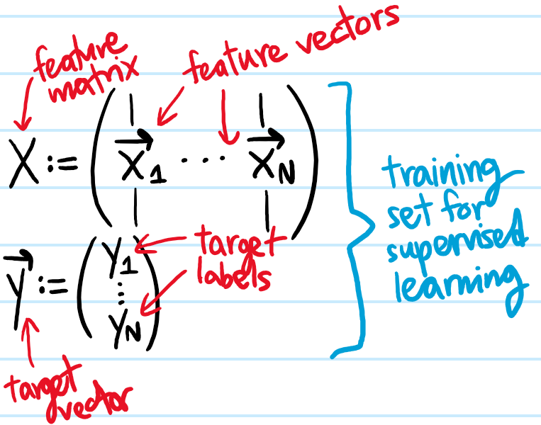
In unsupervised learning, the machine is simply given a bunch of feature vectors \(\textbf x_1,…,\textbf x_N\) without being labelled by any target values, and asked to find patterns/structure within the data. Thus, supervision and training are synonymous.
Problem: What does the manifold hypothesis state?
Solution: The manifold hypothesis states that for many machine learning systems, not all of \(n\)-dimensional feature space \(\mathbf R^n\) need be understood, but only some submanifold \(\cong\mathbf R^{n’}\) of dimension \(n'<n\). This partially offsets the curse of dimensionality.
Problem: What are the \(2\) most common types of supervised learning?
Solution: If the range of target labels \(y_i\) is at most countable (e.g \(\{0,1\},\textbf N,\textbf Q\), etc.) then this type of supervised learning is called classification (in the special case of \(\{0,1\}\), this is called binary classification whereas beyond \(2\) target labels it would be called multiclass classification). If instead the range of target labels \(y_i\) is uncountable (e.g. \(\textbf R,\textbf C\)) then this type of supervised learning is called regression (cf. the distinction between discrete and continuous random variables).
Problem: Write down the normal equations for multivariate linear regression, and the corresponding optimal estimators.
Solution: Given \(N\) labelled training examples \(\{(\mathbf x_1,y_1),…,(\mathbf x_N,y_N)\}\), the goal is to fit a linear map \(\hat y(\mathbf x|\mathbf w)=\mathbf w\cdot\mathbf x\) to the data (each of the \(N\) feature vectors \(\mathbf x_1,…,\mathbf x_N\) should be thought of as appended with a constant feature \(1\) and \(\mathbf w\) being in fact a “weight-bias vector” in the sense that its last entry is the bias \(b\)). Ideally, we would like to find a \(\mathbf w\) such that \(\mathbf w\cdot\mathbf x_1=y_1\),…,\(\mathbf w\cdot\mathbf x_N=y_N\), or in terms of the feature matrix \(X:=(\mathbf x_1,…,\mathbf x_N)\), one would like \(X^T\mathbf w=\mathbf y\) where \(\mathbf y:=(y_1,…,y_N)^T\). However, in general this won’t be possible. Instead, minimizing the MSE cost function:
\[\frac{\partial}{\partial\mathbf w}|\mathbf y-\mathbf X^T\mathbf w|^2=\mathbf 0\]
one obtains the normal equations:
\[XX^T\mathbf w=X\mathbf y\]
and hence, because the Gram matrix \(XX^T\) is positive semi-definite and Hermitian, may be inverted:
\[\mathbf w=X^{T+}\mathbf y\]
where the pseudoinverse \(X^{T+}\) of \(X^T\) is given by:
\[X^{T+}=(XX^T)^{-1}X\]
Problem: Write down the iterative update rule for standard batch gradient descent minimization of an arbitrary real-valued scalar field \(C(\boldsymbol{\theta})\).
Solution: The update rule for \(\partial_{\boldsymbol{\theta}}\)-descent is:
\[\boldsymbol{\theta}\mapsto\boldsymbol{\theta}-\alpha\frac{\partial C}{\partial\boldsymbol{\theta}}\]
where \(\alpha>0\) is a (possibly variable) learning rate.
Problem: In ML applications, \(C(\boldsymbol{\theta})\) has the interpretation of a so-called cost function and the parameters \(\boldsymbol{\theta}\) are usually called weights and biases. What’s special about the ML cost function \(C(\boldsymbol{\theta})\), and how does mini-batch stochastic gradient descent (SGD) exploit this?
Solution: It takes the form of a sum of a bunch of s0-called loss functions. That is:
\[C(\boldsymbol{\theta})=\frac{1}{N}\sum_{i=1}^NL(\mathbf x_i,y_i|\boldsymbol{\theta})\]
which is an expectation over the empirical distribution of the \(N\) training examples \((\mathbf x_1,y_1),…,(\mathbf x_N,y_N)\). Here, the integer \(N\) will be important. A typical supervised ML model might be trained on \(N\sim 10^9\) labelled feature vectors. This means that the corresponding gradient of the cost function:
\[\frac{\partial C}{\partial\boldsymbol{\theta}}=\frac{1}{N}\sum_{i=1}^N\frac{\partial L(\mathbf x_i,y_i|\boldsymbol{\theta})}{\partial\boldsymbol{\theta}}\]
would also require summing \(N\) terms, thus making each step of standard batch \(\partial_{\boldsymbol{\theta}}\)-descent computationally expensive. The idea of mini-batch stochastic gradient descent is to replace \(N\mapsto N'<N\) in order to reduce the computational burden at the expense of throwing away some precision about the optimal direction in \(\boldsymbol{\theta}\)-space to take each \(\partial_{\boldsymbol{\theta}}\)-descent step. Strictly speaking, SGD itself is the extreme limit in which \(N’:=1\), but in practice it is more common to use mini-batch SGD in which say \(N’=10^3\) so that the original ocean of \(N=10^9\) training examples may be randomly partitioned into \(N/N’=10^6\) mini-batches each containing \(N’=10^3\) training examples. Then, the mini-batches are further randomly sampled (with replacement) for each step of this modified/stochastic \(\partial_{\boldsymbol{\theta}}\)-descent:
\[\boldsymbol{\theta}\mapsto\boldsymbol{\theta}-\frac{\alpha}{N’}\sum_{i=1}^{N’}\frac{\partial L(\mathbf x_i,y_i|\boldsymbol{\theta})}{\partial\boldsymbol{\theta}}\]
Problem:
\[C(\textbf w,b):=\frac{1}{2N}\sum_{i=1}^N(\hat{y}(\textbf x_i|\textbf w,b)-y_i)^2\]
is a mean-square cost function for a linear regression model \(\hat y(\textbf x|\textbf w,b)=\textbf w\cdot\textbf x+b\) attempting to predict a training set \(\{(\textbf x_1,y_1),…,(\textbf x_N,y_N)\}\) (here \(\textbf w\) is a weight vector and \(b\) is called a bias), what do the update rules for gradient descent look like in mathematical notation (explicitly)?
Solution: Note that \(\textbf w_n\) and \(b_n\) should be updated simultaneously:
\[\textbf w_n=\textbf w_{n-1}-\frac{\alpha}{N}\sum_{i=1}^N(\textbf w_{n-1}\cdot\textbf x_i+b_{n-1}-y_i)\textbf x_i\]
\[b_n=b_{n-1}-\frac{\alpha}{N}\sum_{i=1}^N(\textbf w_{n-1}\cdot\textbf x_i+b_{n-1}-y_i)\]
Problem: What are the \(2\) key advantages of using NumPy?
Solution:
- Advantage #\(1\): Vectorization. The reason this is classified as an advantage hinges on the premise that modern parallel computing hardware (e.g. GPUs) turned out (somewhat unintentionally) to very efficient at matrix multiplication (and more broadly the many standard operations on/between NumPy arrays). The smoking gun for a correctly vectorized implementation of a computer program is that there should be no Python for loops visible anywhere in the code; all should instead be swept under the NumPy rug.
- Advantage #\(2\): Broadcasting. This allows standard operations such as scalar multiplication \(\textbf x\mapsto c\textbf x\) to occur.
Universal functions (ufuncs) in NumPy (precompiled \(C\)-loop).
(crudely speaking, these are Cartesian tensors in math/physics). Typically never have to bother with Python loops.
Problem: Implement gradient descent in Python for the training set \(\{(1,1),(2,2),(3,3)\}\) using a linear regression model. In particular, for a fixed initial guess, determine the optimal learning rate \(\alpha\). Also try different initial guesses? And batch gradient descent vs. mini-batch…
Solution:
$\textbf{Problem}$: Write Python code to generate two random vectors $\textbf w,\textbf x\in\mathbf R^{10^7}$ and compute their dot product $\textbf w\cdot\textbf x$:
i) Without vectorization (i.e. using a for loop)
ii) With vectorization
Show that vectorization significantly speeds up the computation of $\textbf w\cdot\textbf x$.
$\textbf{Solution}$:
import numpy as np # import the NumPy library
from numpy import random # import the random module from the NumPy library
from time import time # import the time library

n = int(1e7)
random.seed(62831853) # seed for "predictable" random vectors
w = random.rand(n) # random vector with n entries between 0 and 1
print(w)
x = random.rand(n) # random vector with n entries between 0 and 1
print(x)

# Without vectorization:
t_initial = time()
dot_product = 0
for i in np.arange(n):
    dot_product = dot_product + w[i]*x[i]
t_final = time()
print(f"Dot product value: {dot_product}")
print(f"Time taken: {t_final-t_initial} seconds")

# With vectorization:
t_initial = time()
dot_product = np.dot(w,x)
t_final = time()
print(f"Dot product value: {dot_product}")
print(f"Time taken: {t_final-t_initial} seconds")
[0.99139118 0.98259778 0.04074994 ... 0.37571015 0.46541306 0.60192845]
[0.02930771 0.23935712 0.46679807 ... 0.67633435 0.5376593  0.09256103]
Dot product value: 2499560.663731212
Time taken: 4.61395788192749 seconds
Dot product value: 2499560.663731507
Time taken: 0.003765106201171875 seconds
$\textbf{Problem}$:
i) Generate (from a fixed seed) $1000$ random points in the $xy$-plane which are dispersed around the line $y=3x+1$ with standard deviation $\sigma_y=50$, in the range $0\leq x\leq 100$.
ii) Using the univariate linear regression model $\hat y=wx+b$ with initial guess $w=b=0$, apply gradient descent with learning rates $\alpha=10^{-6},10^{-5},10^{-4}$ for $100$ iterations each and plot the corresponding learning curves.
iii) Show, for each of the previous values of $\alpha$, the machine learning of $(w,b)$ in a suitable plane.
$\textbf{Solution}$:
import numpy as np
import matplotlib.pyplot as plt
import scienceplots

N = 1000
x_min = 0
x_max = 100
sigma_y = 50

rng = np.random.default_rng(seed=62831853)
x = np.array(rng.uniform(x_min, x_max, N))
y = np.array(3*x + 1 + rng.normal(0, sigma_y, N))

with plt.style.context(['science']):
    plt.figure(figsize=(10, 5))
    plt.scatter(x, y, s=0.5)
    plt.title("Random Data")
    plt.xlabel(r"$x$")
    plt.ylabel(r"$y$")
    plt.show()

def y_hat(x, w, b):
    return w[..., None] * x + b[..., None]

def C(x, y, w, b):
    return 0.5 * np.mean((y_hat(x, w, b) - y)**2, axis=-1)

def dC_dw(w, b):
    return 1/N * np.sum((y_hat(x, w, b) - y) * x, axis=-1)

def dC_db(w, b):
    return 1/N * np.sum(y_hat(x, w, b) - y, axis=-1)

def grad_descent(w_init, b_init, alpha, n):
    w = np.zeros(n)
    b = np.zeros(n)
    w[0] = w_init
    b[0] = b_init
    for i in np.arange(1, n):
        w[i] = w[i-1] - alpha * dC_dw(w[i-1], b[i-1])
        b[i] = b[i-1] - alpha * dC_db(w[i-1], b[i-1])
    return w, b
n = 100
w_init = 0
b_init = 0

iterations = np.arange(n)
costs = np.zeros(n)

with plt.style.context(['science']):
    plt.figure(figsize=(10, 5))
    for alpha in [1e-6, 1e-5, 1e-4]:
        w, b = grad_descent(w_init, b_init, alpha, n)
        plt.plot(iterations, C(x, y, w, b), label=r"$\alpha=$"+str(alpha))
    plt.title("Learning Curves for Gradient Descent for Several Learning Rates")
    plt.xlabel("Number of Iterations")
    plt.ylabel("Cost Function")
    plt.legend()
    plt.show()

with plt.style.context(['science']):
    plt.figure(figsize=(10, 5))
    for alpha in [1e-6, 1e-5, 1e-4]:
        weights, biases = grad_descent(w_init, b_init, alpha, n)
        plt.scatter(weights, biases, label=r"$\alpha=$"+str(alpha), s=0.5)
    plt.title(r"Machine Learning the Linear Regression Model Parameters $w,b$")
    plt.xlabel(r"$w$")
    plt.ylabel(r"$b$")
    plt.legend()
    plt.show()

Problem: Explain how feature normalization and feature engineering can help to speed up gradient descent and obtain a model with greater predictive power.
Solution: Because the learning rate \(\alpha\) in gradient descent is, roughly speaking, a dimensionless parameter, it makes sense to nondimensionalize all feature variables in some sense. This is the idea of feature normalization. For instance, one common method is to simply perform range normalization:
\[x\mapsto\frac{x-\langle x\rangle}{\text{range}(x)}\]
Another method is standard deviation normalization where instead of using the range as a crude measure of dispersion, one replaces it by the more refined standard deviation to obtain a \(z\)-score:
\[x\mapsto\frac{x-\langle x\rangle}{\sigma_x}\]
Feature engineering is about using one’s intuition to design new features by transforming or combining original features. Typically, this means expanding the set of basis functions one works with, thus allowing one to curve fit even for nonlinear functions. Thus, linear regression also works with nonlinear functions; the word “linear” in “linear regression” shouldn’t be thought of as “linear fit” but as “linear algebra”.
Problem: Now consider the other type of supervised learning, namely classification, and specifically consider the method of logistic classification (commonly called by the misnomer of logistic “regression” even though it’s about classification). Write down a table comparing linear regression with logistic classification with regards to their:
i) Model function \(\hat y(\textbf x|\textbf w,b)\) to be fit to the training set \(\{(\textbf x_1,y_1),…,(\textbf x_N,y_N)\}\).
ii) Loss functions \(L(\hat y,y)\) appearing in the cost function \(C(\textbf w,b)=\frac{1}{N}\sum_{i=1}^NL(\hat y(\textbf x_i|\textbf w,b),y_i)\).
Solution:
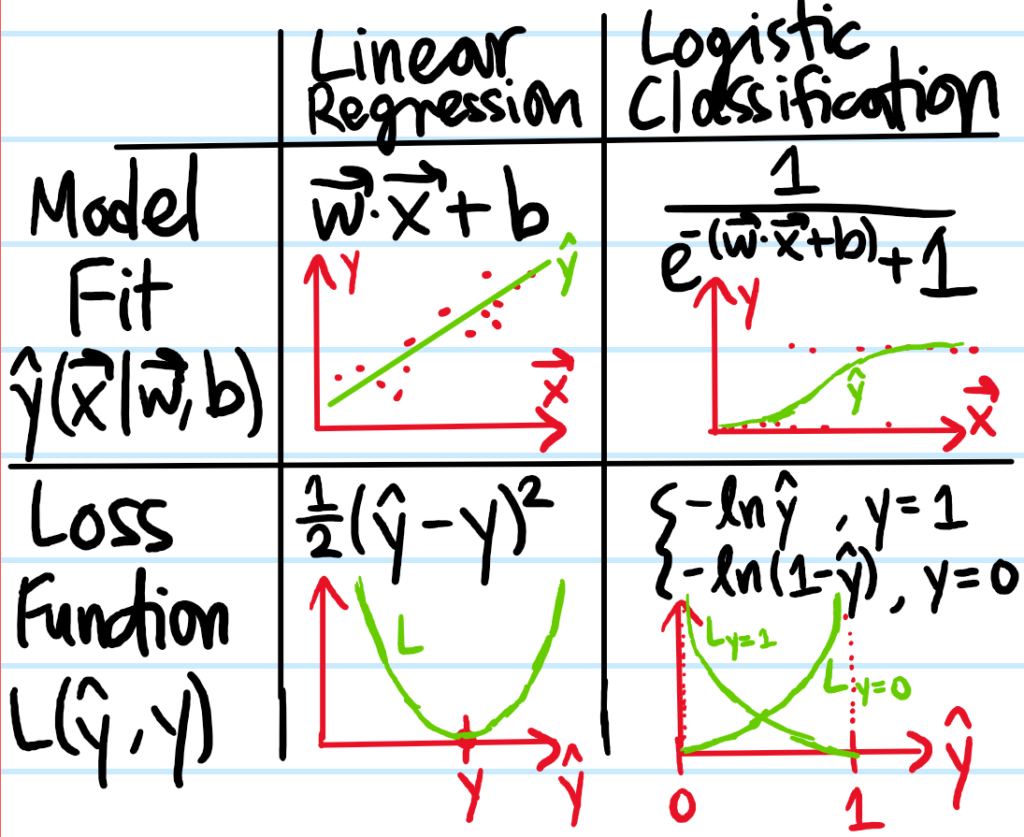
where, as a minor aside, the loss function for logistic classification can also be written in the explicit “Pauli blocking” or “entropic” form:
\[L(\hat y,y)=-y\ln\hat y-(1-y)\ln(1-\hat y)\]
Indeed, it is possible to more rigorously justify this choice of loss function precisely through such maximum-likelihood arguments. For simplicity, one can simply think of this choice of \(L\) for logistic classification as ensuring that the corresponding cost function \(C\) is convex so that gradient descent can be made to converge to a global minimum (which wouldn’t have been the case if one had simply stuck with the old quadratic cost function from linear regression). A remarkable fact (related to this?) is that the explicit gradient descent update formulas for each iteration look exactly the same for linear regression and logistic classification:
\[\textbf w_n=\textbf w_{n-1}-\frac{\alpha}{N}\sum_{i=1}^N(\hat y(\textbf x_i|\textbf w_{n-1},b_{n-1})-y_i)\textbf x_i\]
\[b_n=b_{n-1}-\frac{\alpha}{N}\sum_{i=1}^N(\hat y(\textbf x_i|\textbf w_{n-1},b_{n-1})-y_i)\]
just with the model function \(\hat y(\textbf x|\textbf w,b)\) specific to each case.
Problem: Given a supervised classification problem involving some training set to which a logistic sigmoid is fit with some optimal weights \(\textbf w\) and bias \(b\), how does the actual classification then arise?
Solution: One has to decide on some critical “activation energy”/threshold \(\hat y_c\in[0,1]\) such that the classification of a (possibly unseen) feature vector \(\textbf x\) is \(\Theta(\hat y(\textbf x|\textbf w,b)-\hat y_c)\in\{0,1\}\). Thus, the set of feature vectors \(\textbf x\) for which \(\hat y(\textbf x|\textbf w,b)=\hat y_c\) is called the decision boundary.
Problem: Given \(N\) feature vectors \(\mathbf x_1,…,\mathbf x_N\in\mathbf R^n\) each with \(n\) features, explain the curse of dimensionality relating the \(2\) integers \(N\) and \(n\), and methods for addressing it.
Solution: As the number of features \(n\) increases, the corresponding number of feature vectors \(N\) required for the ML model to generalize accurately grows exponentially:
\[N\sim\exp(n)\]
This is simply due to the fundamental geometric sparseness of higher-dimensional Euclidean space \(\mathbf R^n\). Thus, any method for addressing the curse of dimensionality must either increase \(N\) (collect more training examples!) or decrease \(n\) (either blunt feature selection or more sophisticated feature engineering using \(n\)-reduction techniques like PCA).
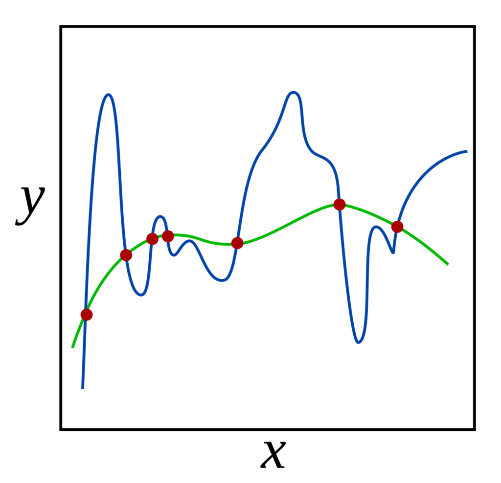
Problem: Explain what it means to regularize a learning algorithm. Give examples of regularization techniques.
Solution: In the broadest sense, regularizing a learning algorithm means making some tweak to the algorithm so as to reduce its tendency to overfit to the training data. More precisely, the goal of regularization is to reduce the model’s effective capacity (though not its representational capacity) in such a way that there would be a substantial decrease in the model’s variance that more than offsets a slight increase in bias. This thereby reduces the overall generalization error of the model, without significantly increasing its training error.
Examples of regularization include \(L^1\) (Lasso) regularization in which the cost function \(C(\mathbf w,b)\) acquires an additional penalty term of the form:
\[C(\textbf w,b)\mapsto C(\textbf w,b)+\frac{\lambda_1}{2N}|\textbf w|\]
or \(L^2\) (ridge) regularization in which:
\[C(\textbf w,b)\mapsto C(\textbf w,b)+\frac{\lambda_2}{2N}|\textbf w|^2\]
(this one actually has an interpretation as arising from a Bayesian MAP estimate assuming an isotropic zero-mean normally distributed prior \(p(\mathbf w)=\left(\frac{\lambda}{2\pi}\right)^{n/2}e^{-\lambda |\mathbf w|^2/2}\)).
Of course, other regularization techniques (both explicit like above and implicit) exist.
(optionally though not typically one can also regularize the bias term \(b\) by adding \(\lambda b^2/2N\) to the cost function \(C\)). Here, \(\lambda_1,\lambda_2\) like \(\alpha\) is another hyperparameter (sometimes called a regularization parameter).