
Problem: What is the defining property of the (Cauchy) stress tensor (field) \(\sigma(\textbf x,t)\) of a material.
Solution: The idea is that if one wants to find the stress vector (also called traction) \(\boldsymbol{\sigma}\) acting on a plane with unit normal \(\hat{\textbf n}\) in the material at location \(\textbf x\) and time \(t\), then this is obtained by acting with the stress tensor:
\[\boldsymbol{\sigma}=\sigma\hat{\textbf n}\]
Or in components:
\[\sigma_i=\sigma_{ij}n_j\]
Problem: What do the diagonal stresses \(\sigma_{11},\sigma_{22},\sigma_{33}\) represent physically? What about the off-diagonal stresses \(\sigma_{12},\sigma_{23},\sigma_{13}\), etc.
Solution: The diagonal stresses represent normal stresses. The off-diagonal stresses represent shear stresses.
Problem: Under what conditions is the stress tensor \(\sigma^T=\sigma\) symmetric? What does this imply the existence of?
Solution: Provided the net couple/torque vanishes \(\boldsymbol{\tau}=\textbf 0\) (intuitively, the normal stresses do not supply any torque, it is the off-diagonal shear stresses that need to match to ensure this rotational equilibrium).
The immediate corollary of this is that, as usual, \(\sigma\) will have \(3\) orthogonal eigenspaces (called principal directions spanned by \(\hat{\textbf n}\), whose orthogonal complements \(\text{span}^{\perp}(\hat{\textbf n})\) are called the principal planes) each associated to a real eigenvalue (called a principal stress). Physically, the stress vector \(\boldsymbol{\sigma}\) acts perpendicularly to such principal planes along the principal directions, so it is a pure normal stress since when diagonalized the off-diagonal shear stresses vanish.
Problem: If \(\sigma_{1,2,3}\) is a principal stress of the stress tensor \(\sigma\), explain why:
\[\sigma_{1,2,3}^3-\text{Tr}(\sigma)\sigma_{1,2,3}^2+\frac{1}{2}\left(\text{Tr}^2(\sigma)-\text{Tr}(\sigma^2)\right)\sigma_{1,2,3}-\det(\sigma)=0\]
Solution: This is a bit trivial in that it’s just the general form of the characteristic equation for any \(3\times 3\) matrix. Equally trivial is the fact that coefficients are coordinate-free (and sometimes called stress invariants in this context). In terms of the principal stresses \(\sigma_1,\sigma_2,\sigma_3\) at a given point in spacetime (not to be confused with the components of the stress vector), of course one has:
\[\text{Tr}(\sigma)=\sigma_1+\sigma_2+\sigma_3\]
\[\frac{1}{2}\left(\text{Tr}^2(\sigma)-\text{Tr}(\sigma^2)\right)=\sigma_1\sigma_2+\sigma_2\sigma_3+\sigma_3\sigma_1\]
\[\det(\sigma)=\sigma_1\sigma_2\sigma_3\]
Problem: Suppose one were interested in just the normal stress in the direction \(\hat{\textbf n}\) at some point even though the stress vector \(\boldsymbol{\sigma}\) was not parallel with \(\hat{\textbf n}\) (i.e. not a principal direction!). How can one nevertheless extract this information?
Solution: Do the obvious thing \(\hat{\textbf n}\cdot\boldsymbol{\sigma}=\hat{\textbf n}^T\sigma\hat{\textbf n}=\sigma_{ij}n_in_j\).
Problem: (Mohr’s circle, (equivalent) von Mises stress, yield criteria, cool Lagrange multiplier optimization problem for max/min shear stresses in Tresca’s criterion)
Solution:
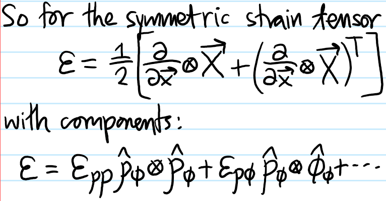
Problem: What is the definition of the strain tensor \(\varepsilon\)?
Solution: It is the symmetric part of the Jacobian of the displacement field \(\textbf X(\textbf x,t)\), i.e.
\[\varepsilon:=\frac{1}{2}\left(\frac{\partial}{\partial\textbf x}\otimes\textbf X+\left(\frac{\partial}{\partial\textbf x}\otimes\textbf X\right)^T\right)\]
Or with respect to a Cartesian basis:
\[\varepsilon_{ij}=\frac{1}{2}\left(\partial_i X_j+\partial_j X_i\right)\]
and therefore is by construction symmetric \(\varepsilon^T=\varepsilon\).
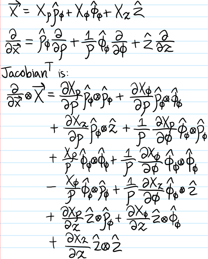
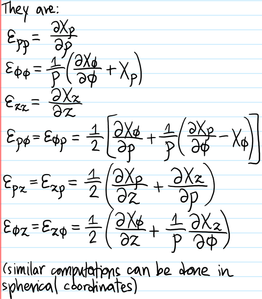
Problem: Find the components of the strain tensor \(\varepsilon\) in cylindrical coordinates.
Solution:
Problem: Describe the grown-up version of Hooke’s constitutive law relating \(\varepsilon\) to \(\sigma\).
Solution: At its essence, Hooke’s law postulates there exists a linear and elastic (i.e. in thermodynamics language, reversible, i.e. no hysteresis) relationship between them, given by a rank-\(4\) tensor field \(C\) (called the elasticity/stiffness tensor):
\[\sigma=C\varepsilon\]
Or, more transparently in Cartesian components:
\[\sigma_{ij}=C_{ijk\ell}\varepsilon_{k\ell}\]
Although a general rank-\(4\) tensor in \(3\)D has \(3^4=81\) degrees of freedom, the symmetries \(\sigma_{ij}=\sigma_{ji}\) and \(\varepsilon_{ij}=\varepsilon_{ji}\) means that \(C_{ijk\ell}=C_{jik\ell}\) and \(C_{ijk\ell}=C_{ij\ell k}\) so the first \(2\) indices \(\{i,j\}\) should be viewed as a multiset rather than an ordered pair, and similarly for the last \(2\) indices \(\{k,\ell\}\). By inspection, there are \(3+2-1\choose{2}\)\(=6\) such multisets, for a total of \(6^2=36\) degrees of freedom. However, the existence of a scalar elastic strain energy density \(\frac{1}{2}C_{ijk\ell}\varepsilon_{ij}\varepsilon_{k\ell}\) means that \(C_{ijk\ell}=C_{k\ell ij}\), so a \(6\times 6\) symmetric matrix has \(\frac{6\times 7}{2}=21\) independent degrees of freedom.
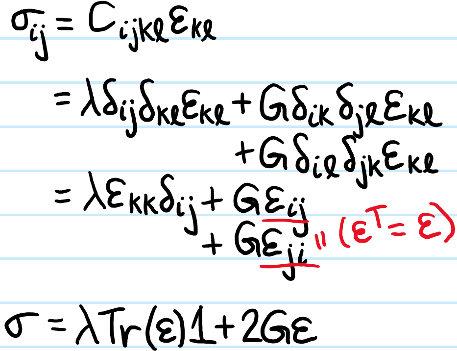
Problem: Imposing further the assumption that \(C\) is an isotropic tensor, explain why \(21\) degrees of freedom are reduced to just \(2\):
\[C_{ijk\ell}=\lambda\delta_{ij}\delta_{k\ell}+G(\delta_{ik}\delta_{j\ell}+\delta_{i\ell}\delta_{jk})\]
where the scalars \(\lambda,G\in\textbf R\) are called the Lame parameters of \(C\).
Solution: A standard mathematical theorem is that the most general form of a rank-\(4\) isotropic tensor is:
\[C_{ijk\ell}=\lambda\delta_{ij}\delta_{k\ell}+\mu\delta_{ik}\delta_{j\ell}+G\delta_{i\ell}\delta_{jk}\]
except that in this case the additional symmetries mentioned earlier (e.g. \(\sigma^T=\sigma\)) enforce \(\mu=G\).
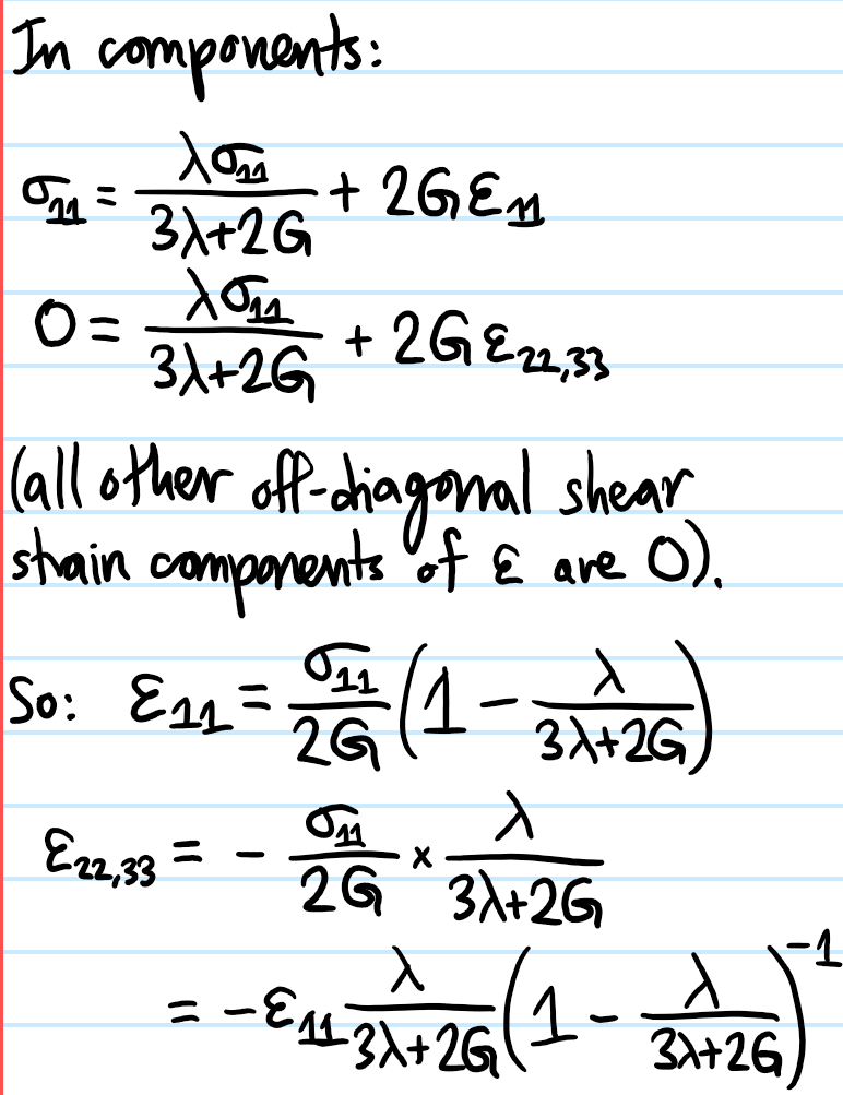
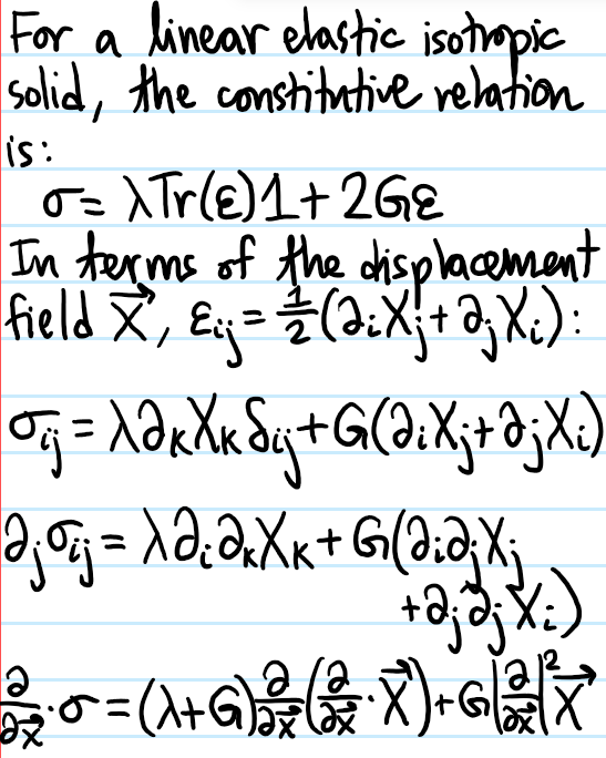
Problem: Hence, demonstrate that for a linear-elastic isotropic material:
\[\sigma=\lambda\text{Tr}(\varepsilon)1+2G\varepsilon\]
Solution: Start with Hooke’s law for a linear-elastic material, and then inject isotropy into \(C\):
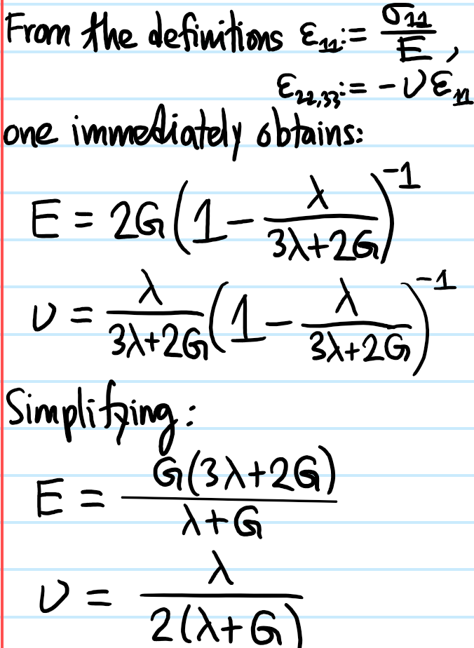
Problem: It is important to emphasize the number “\(2\)” in the statement “there are \(2\) Lame parameters \(\lambda, G\)”. Just as in the thermodynamics of a gas the state of the system is completely specified by \((p,V)\), similarly here any linear-elastic isotropic material’s behavior is completely specified by \(2\) independent moduli, such as \((\lambda, G)\). However, there are also other pairs of moduli available, such as \((E,\nu)\) (Young’s modulus with Poisson’s ratio) or \((B, G)\) (bulk modulus and shear modulus).
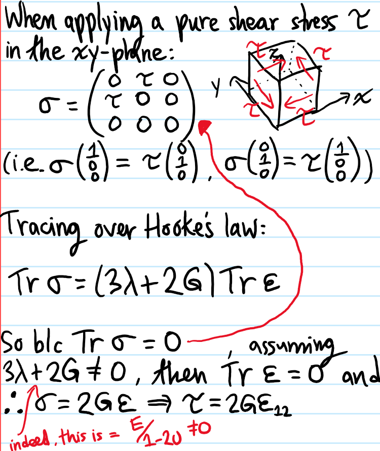
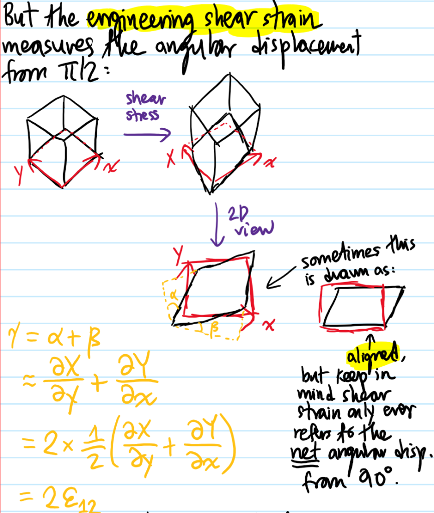
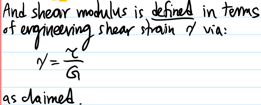
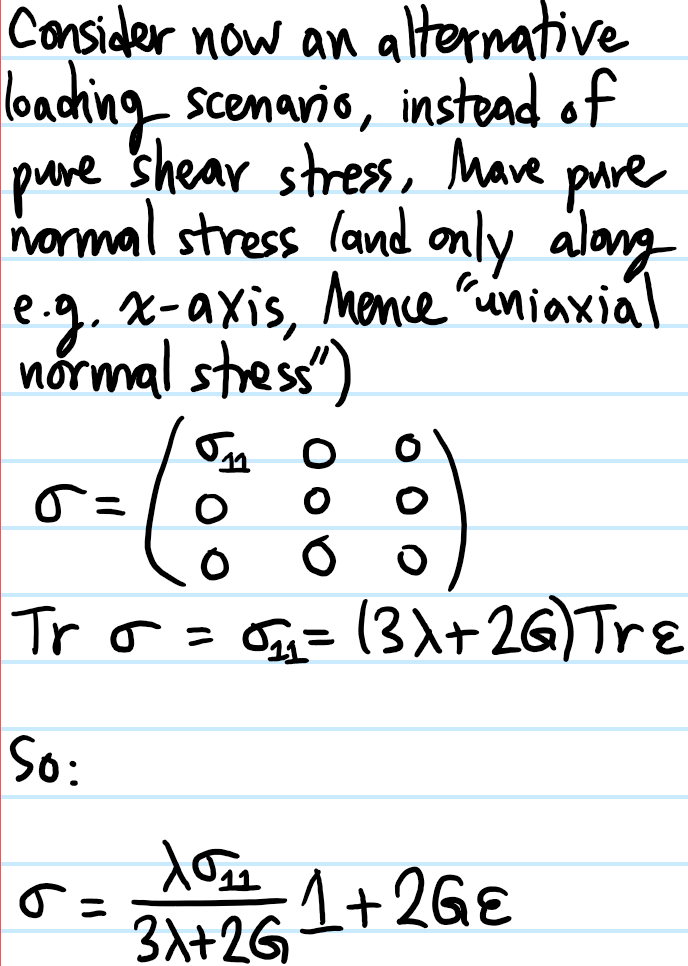
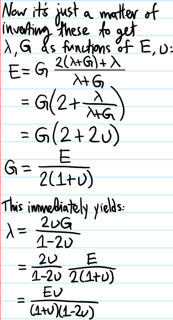
First, explain why the \(G\) here really deserves to be called “shear modulus”. Similarly, by considering other loading scenarios, show that the relevant “Legendre transformations” between the moduli are:
\[\lambda=\frac{E\nu}{(1+\nu)(1-2\nu)}\]
\[G=\frac{E}{2(1+\nu)}\]
\[B=\frac{E}{3(1-2\nu)}\]
Solution:
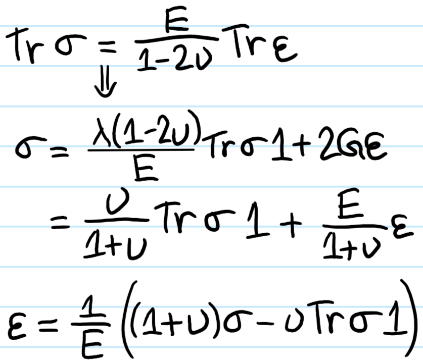
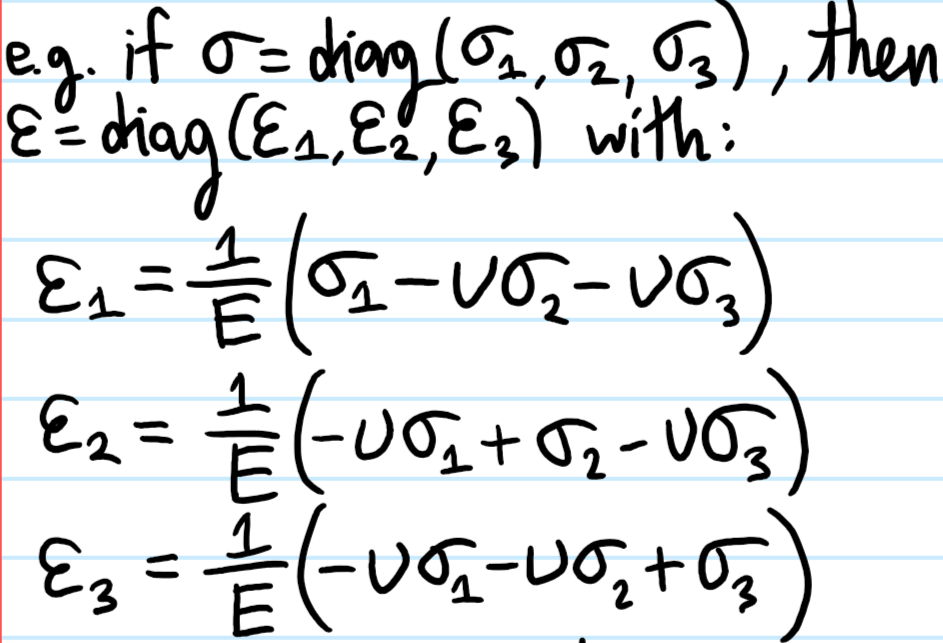
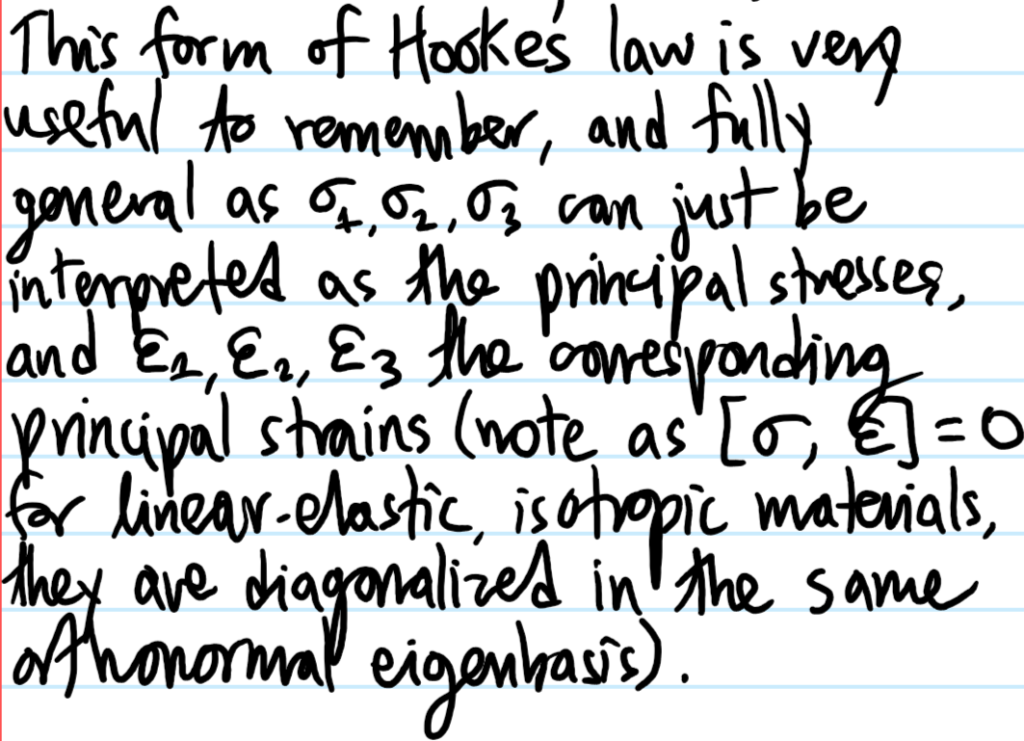
Problem: Hooke’s law for linear-elastic materials as it’s currently written:
\[\sigma=\lambda\text{Tr}(\varepsilon)1+2G\varepsilon\]
conflates cause-and-effect since \(\sigma\) is what causes \(\varepsilon\). Show how to isolate for \(\varepsilon\) in terms of \(\sigma\), and write the resultant Hooke’s law in the principal frame.
Solution:
Problem: Looking at the expression for the bulk modulus \(B\) in terms of \(E\) and \(\nu\):
\[B=\frac{E}{3(1-2\nu)}\]
Explain why this constrains \(\nu\leq 1/2\). What does it mean for a material (e.g. rubber) to have \(\nu=1/2\)?
Solution: Stability requires that \(B\geq 0\) (otherwise one would get a positive feedback loop between \(p,V\)), so this implies \(\nu\leq 1/2\). Materials with \(\nu=1/2\) are volume-preserving; stretching in \(z\) will causes a contraction in \(\rho\) such that \(z\rho^2=\text{const}\). Of course this means the bulk modulus is \(B=\infty\).
Problem: How is this grown-up version of Hooke’s law related to the childish version \(F=-kx\)?
Solution: For a spring of material with Young’s modulus \(E\), wire of cross-section \(A\), and length \(L\), the spring constant is:
\[k=\frac{EA}{L}\]
this should be compared with a similar formula for capacitance of a parallel-plate capacitor:
\[C=\frac{\varepsilon A}{d}\]
or inductance of a long solenoid:
\[L=\frac{\mu N^2A}{\ell}\]
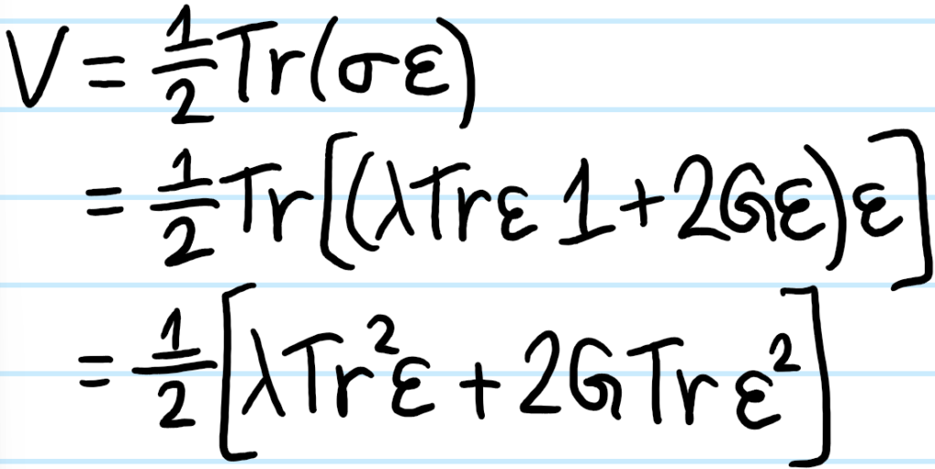
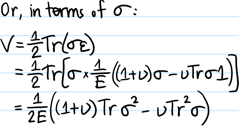
Problem: Explain why, as claimed earlier, for any (possibly anisotropic) linear elastic material, the strain energy density \(V\) is given by:
\[V=\frac{1}{2}C_{ijk\ell}\varepsilon_{ij}\varepsilon_{k\ell}=\frac{1}{2}\text{Tr}(\sigma\varepsilon)\]
And show how this result specializes to the case of an isotropic linear elastic material.
Solution: Basically just the usual argument of doing some work on a unit cell and equating that with the stored energy; the factor of \(1/2\) is the canonical “area-of-a-triangle” factor that arises due to the linearity of the stress-strain “curve”.
Including the assumption of isotropy:
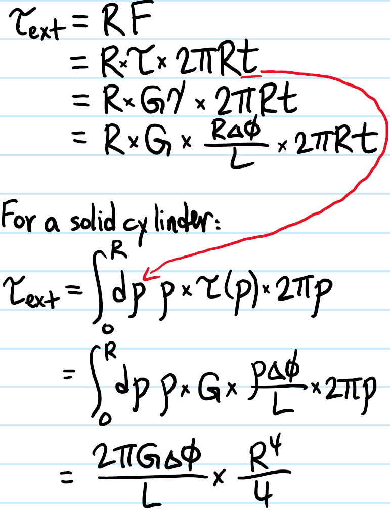
Problem: Consider twisting a hollow cylinder of radius \(R\), length \(L\), and thickness \(t\ll R\) through a small angle \(\Delta\phi\). Show that the external couple \(\tau_{\text{ext}}\) required to maintain this is:
\[\tau_{\text{ext}}=\frac{2\pi GR^3t}{L}\Delta\phi\]
If instead it is a solid cylinder, show that the external couple required is now:
\[\tau_{\text{ext}}=\frac{\pi GR^4}{2L}\Delta\phi\]
(optional: calculate the elastic strain energy stored in the cylinders in both cases).
Solution: 
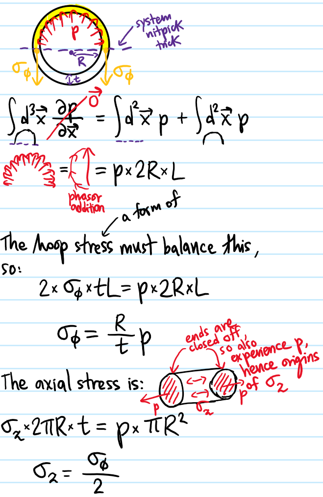
Problem: Consider a uniformly pressurized hollow, capped cylinder of pressure \(p\), radius \(R\), thickness \(t\) and length \(L\). Show that the hoop stress \(\sigma_{\phi}\) and axial stress \(\sigma_z\) are related by a factor of \(2\):
\[\sigma_{\phi}=2\sigma_{z}=\frac{R}{t}p\]
(WHAT ABOUT RADIAL STRESSES \(\sigma_{\rho}\)?)
Solution:
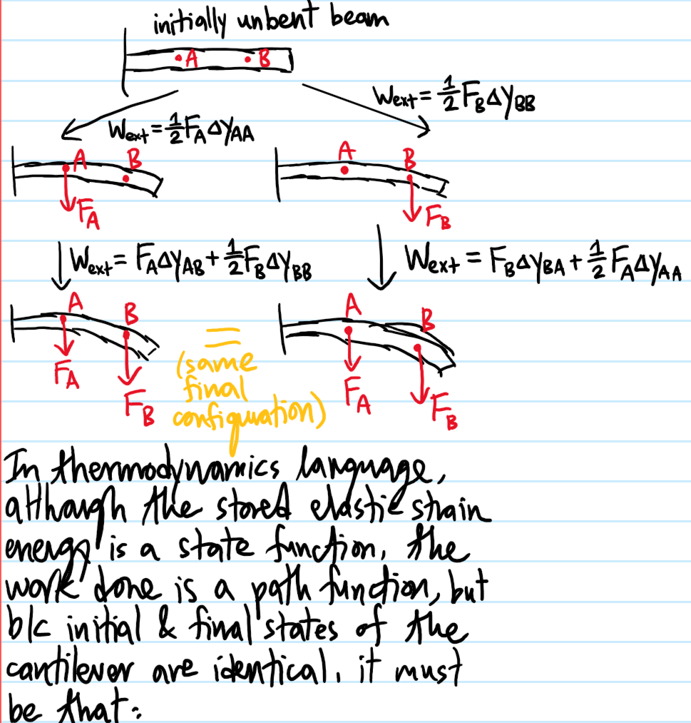
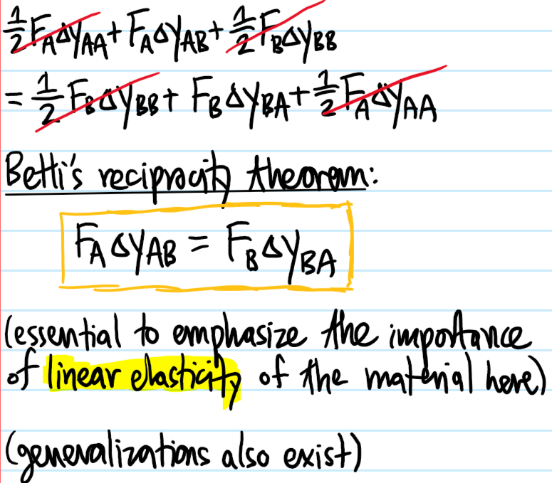
Problem: Demonstrate Betti’s reciprocity theorem for a linear elastic isotropic cantilever beam.
Solution:
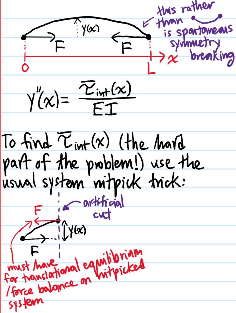
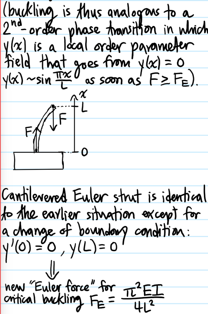
Problem: Show that if one takes a beam with Young’s modulus \(E\), moment of area \(I\), and you start to compress it axially, once the force \(F\) applied exceeds a certain critical force (the “Euler force”), the beam will spontaneously break symmetry by buckling (this configuration is sometimes referred to as the Euler strut).
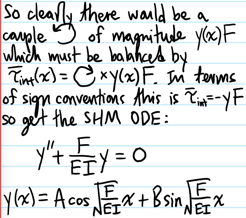
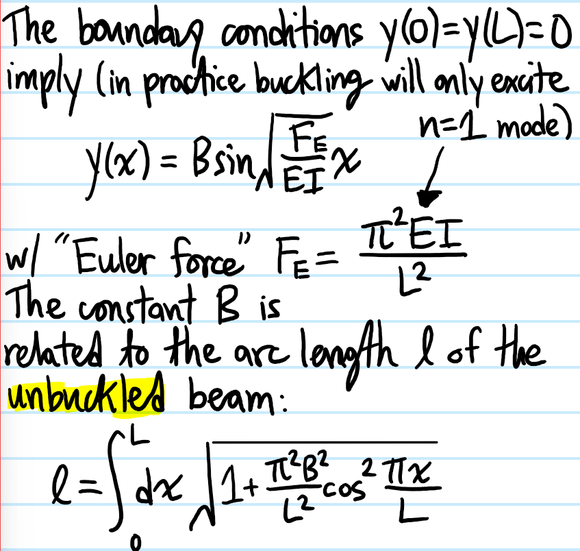
Solution:
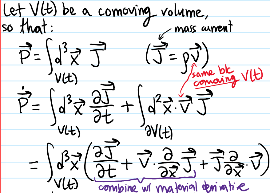
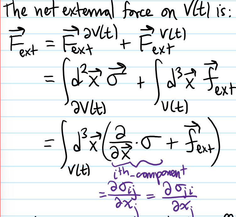
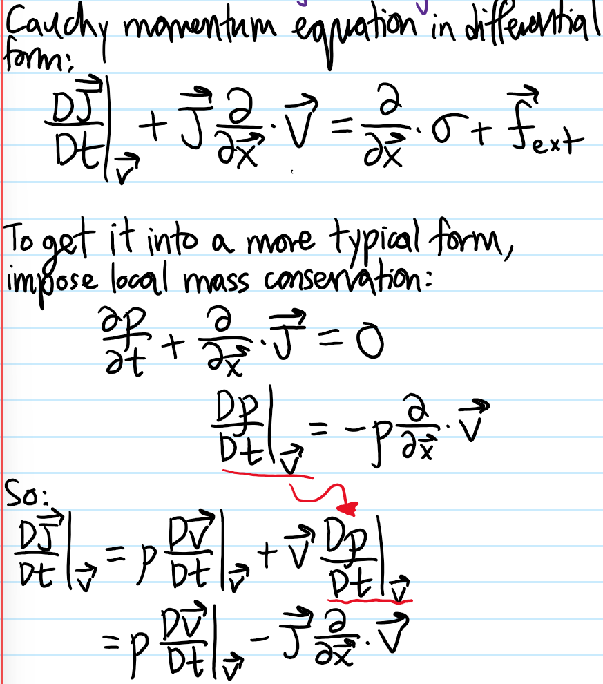
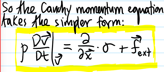
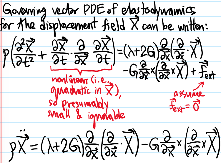
Problem: Show that Newton’s \(2^{\text{nd}}\) law in a continuum becomes the Cauchy momentum equation:
\[\rho\frac{D\textbf v}{Dt}\biggr|_{\textbf v}=\frac{\partial}{\partial\textbf x}\cdot\sigma+\textbf f_{\text{ext}}\]
Solution: Basically just an application of the Reynold’s transport theorem to a system nitpick trick applied to a comoving volume:
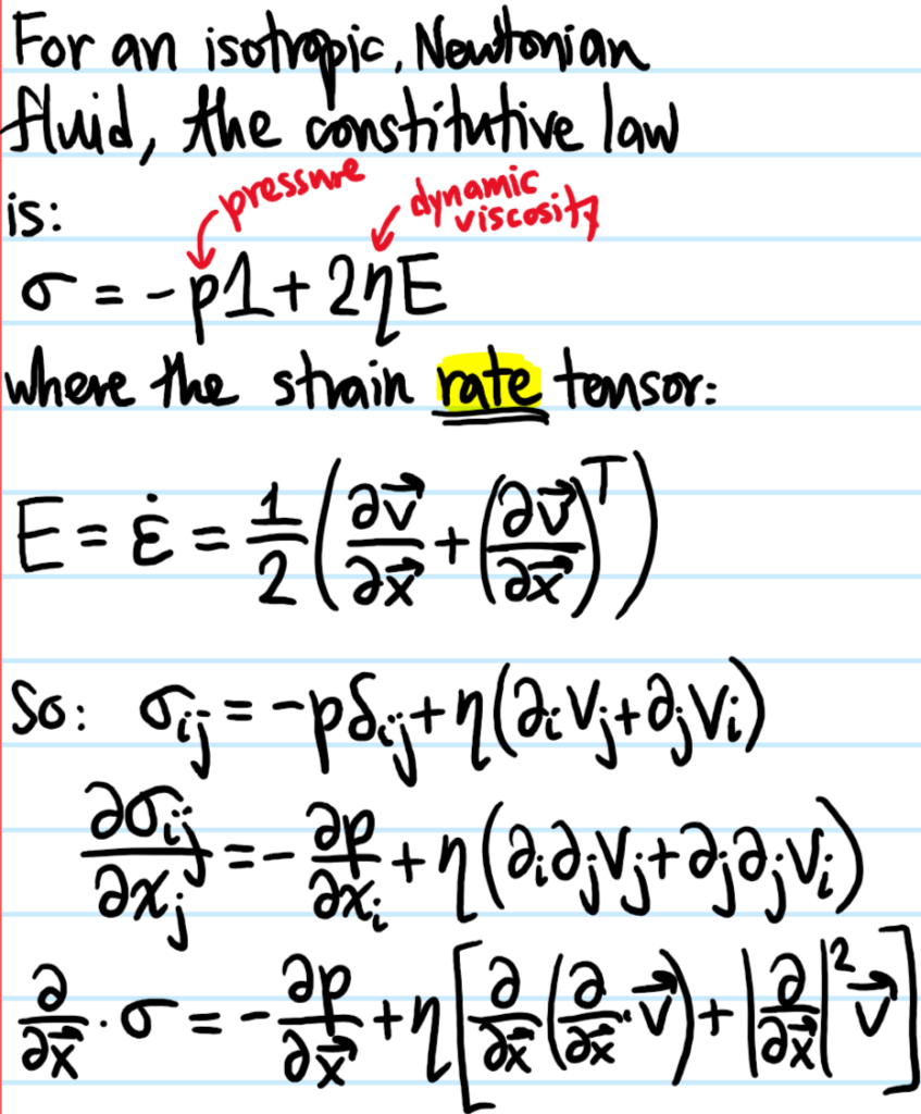
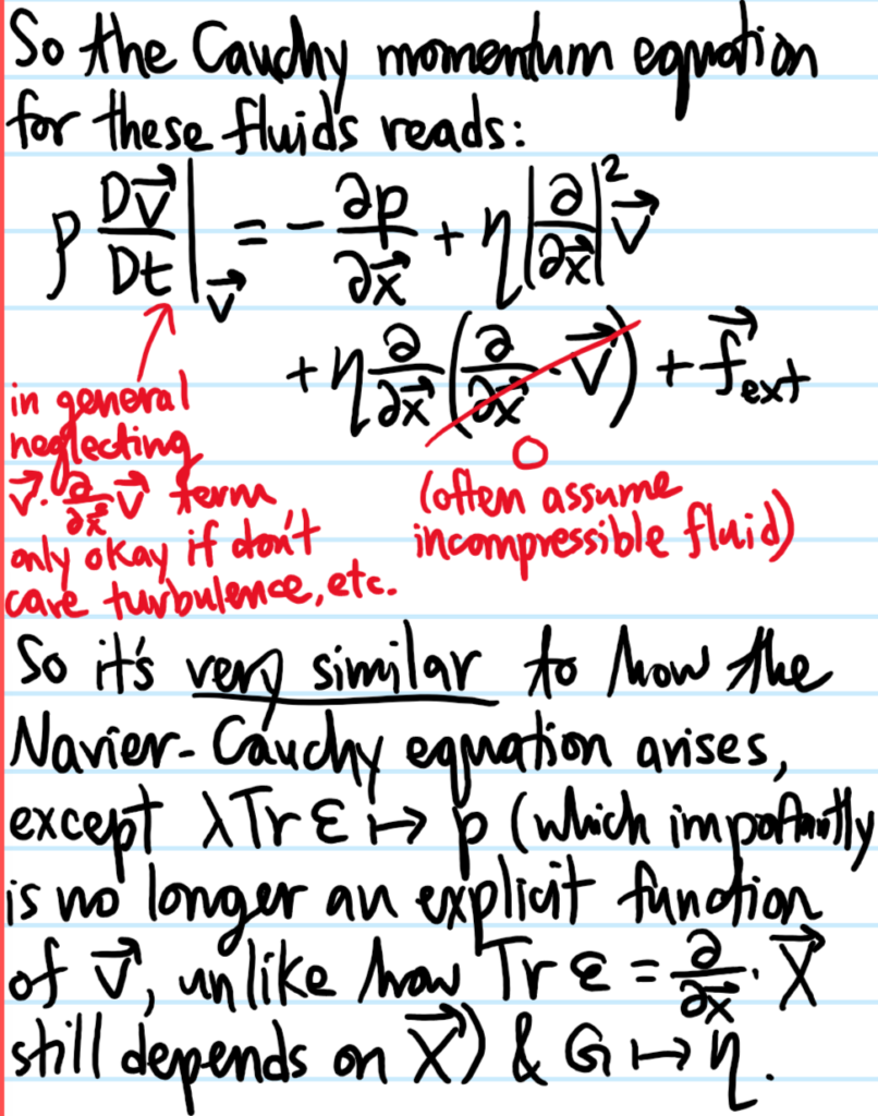
Problem: Show how, using the Cauchy momentum equation as the fundamental starting point, the equations of elastodynamics (Navier-Cauchy equations) and fluid dynamics (Navier-Stokes equations) arise from postulating similar-looking but conceptually different constitutive relations for the stress tensor \(\sigma\).
Solution:
Problem: As the Navier-Cauchy equations are linear, it makes sense to consider a plane wave ansatz \(\textbf X(\textbf x,t)=\textbf X_0e^{i(\textbf k\cdot\textbf x-\omega_{\textbf k}t)}\). Hence show that there are \(2\) kinds of waves:
\[\text{S-waves}\Leftrightarrow\textbf k\cdot\textbf X_0=0\]
\[\text{P-waves}\Leftrightarrow\textbf k\times\textbf X_0=\textbf 0\]
obtain the dispersion relation \(\omega_{\textbf k}\) for \(S\)-waves and \(P\)-waves (cf. \(s\) and \(p\) atomic orbitals or \(s\)-wave and \(p\)-wave scattering in quantum mechanics…the nomenclature is a coincidence as here \(S\) stands for “secondary” while \(P\) stands for “primary”, whereas in the quantum context \(s\) stands for “sharp” while \(p\) stands for “principal”).
Solution:
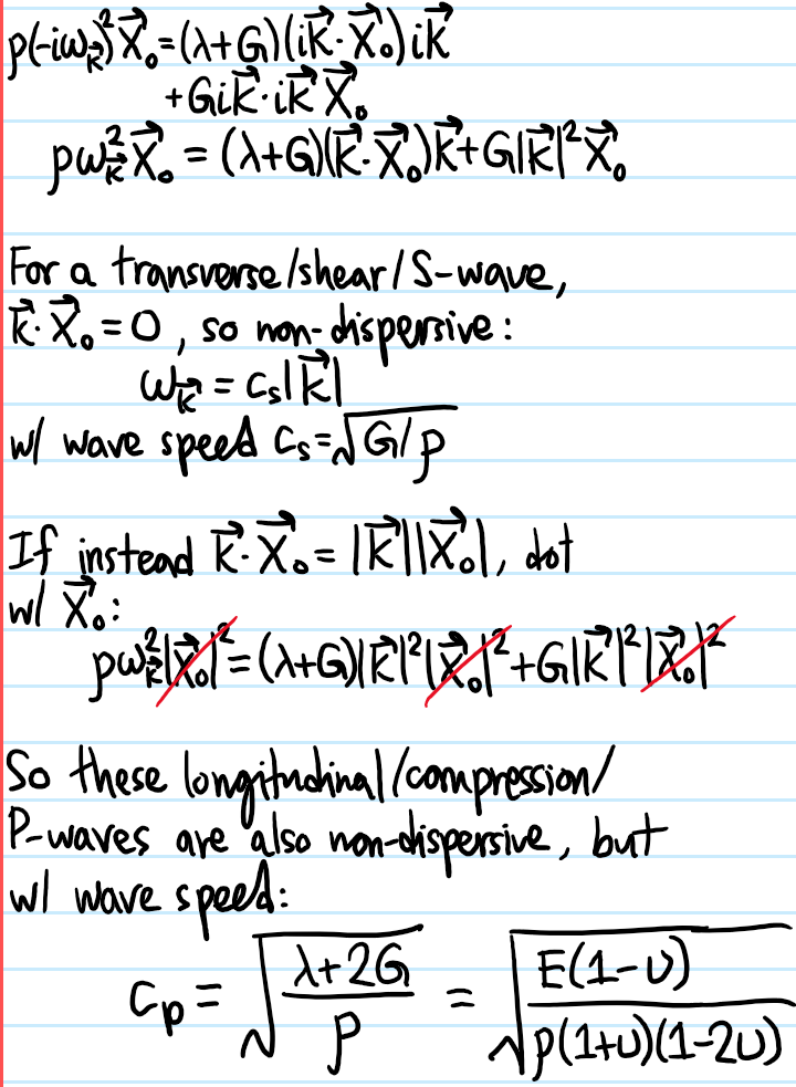
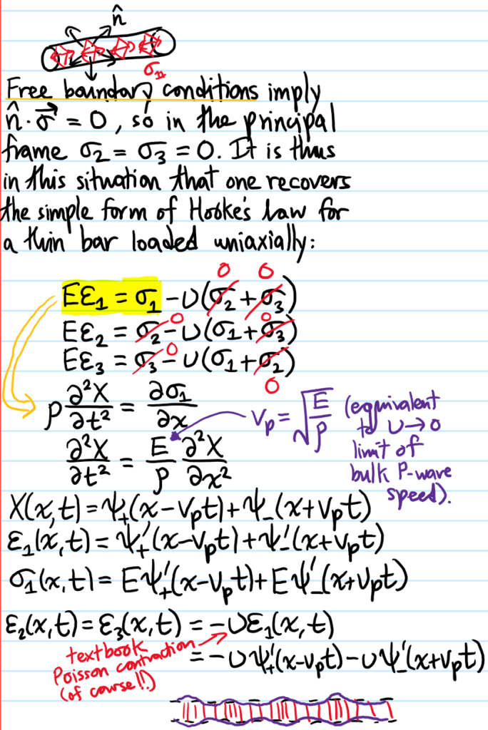
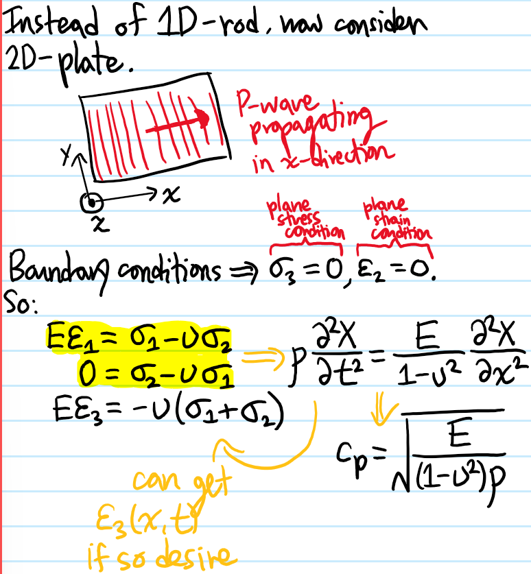
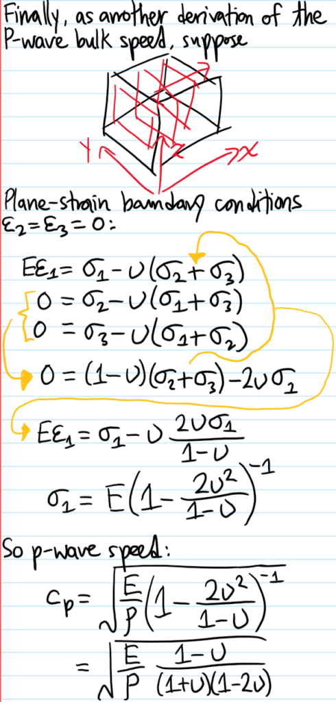
Problem: Consider a longitudinal \(P\)-wave propagating in the \(x\)-direction through:
a) A \(1\)D infinite (linear elastic isotropic) rod.
b) A \(2\)D infinite (linear elastic isotropic) plate.
c) A \(3\)D infinite (linear elastic isotropic) bulk solid.
In each case, what is the speed \(v_p\) of such \(P\)-waves?
Solution:
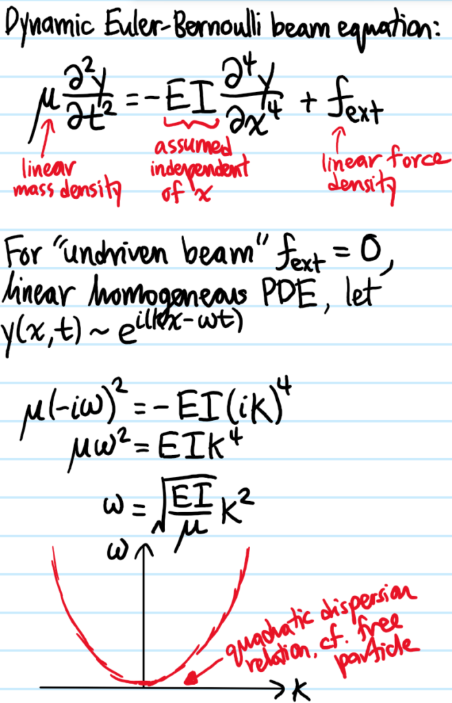
Problem: Starting from the Navier-Cauchy equations, show how to obtain the dynamic Euler-Bernoulli beam equation.
Solution:
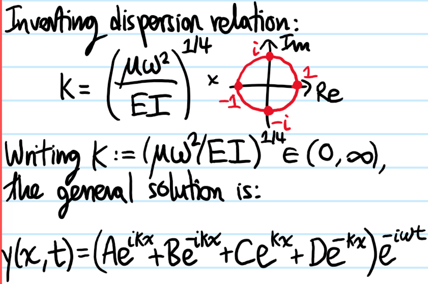
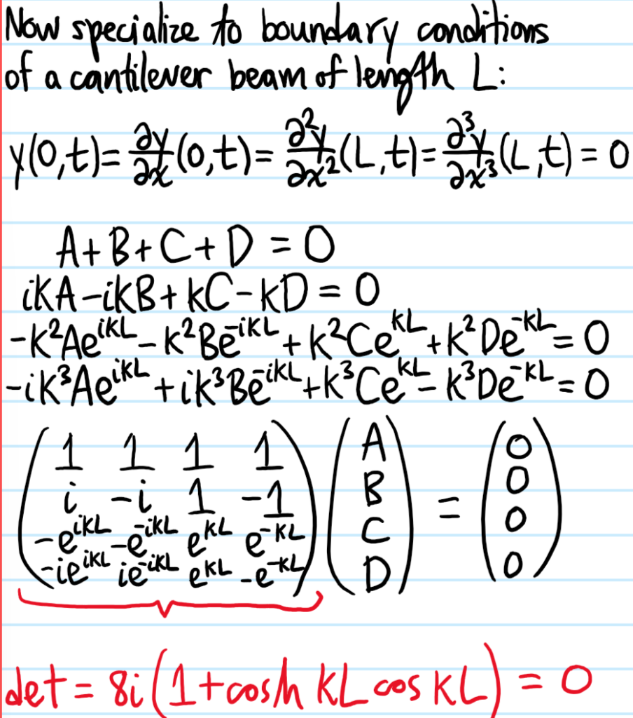
Problem: Find the normal mode frequencies of vibration \(\omega_n\) of a cantilever beam of length \(L\).
Solution:
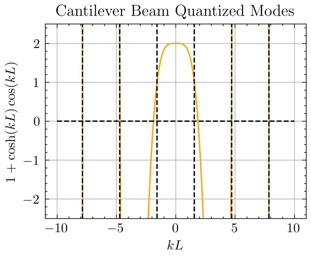
So the allowed values of \(kL\), although strictly given by the zeroes of the graph, quickly tend towards \(k_nL\approx (n+1/2)\pi\) (which are the vertical dashed lines). By the dispersion relation, the corresponding angular frequencies therefore quickly tend toward:
\[\omega_n\approx\sqrt{\frac{EI}{\mu}}\frac{(n+1/2)^2\pi^2}{L^2}\]
Problem: What is the sign convention for the internal couple (also called bending moment) of a beam?
Solution: Remember the mnemonic “top in tension” as this is when \(\bar{\tau}_{\text{int}}(x)>0\). For instance, for a simple cantilever beam drooping under its own weight, the top of the beam is clearly in tension everywhere, so the internal couple will be positive all the way along. Similarly, for a beam which is sagging between \(2\) supports, the top is in compression everywhere so under this sign convention the internal couple is negative everywhere along the beam.
Problem:
The advantage of this convention is that the static Euler-Bernoulli beam equation doesn’t need any pesky minus signs, assuming also the (reasonable) convention that \(y(x)>0\) is an upwards displacement:
\[y”(x)=\bar{\tau}_{\text{int}}(x)/EI\]
Geometrically, it is intuitively clear that when a beam is bent by external forces and torques, some sections will become longer (hence experiencing internal tension) while other sections will become shorter (hence experiencing internal compression). By the intermediate value theorem, there thus exists a section which becomes neither longer nor shorter, instead possessing a bend-invariant length; this is called the neutral axis of the beam (strictly speaking, the neutral axis is not a 1D line, but a 2D surface cutting through the center of the beam so perhaps a better name would have been neutral surface). The neutral axis of the beam therefore experiences neither internal tension nor internal compression, and so is defined by experiencing zero internal stress \(\sigma_{\text{int}}=0\). The idea is to then understand how the internal stress field \(\sigma_{\text{int}}(y)\) varies as a function of the distance \(y\) above (or below) the neutral axis (where we’ve just established it’s zero). Intuitively, this should depend not only on \(y\), but also on the stiffness of the beam material (this is why it’s harder to bend stiffer beams!). Since the internal tensions and internal compressions are essentially uniaxial stresses along the beam, one should invoke Hooke’s law:
$$\sigma_{\text{int}}(y)=E\varepsilon(y)$$
where the engineering strain \(\varepsilon(y)\) at a distance \(y\) from the neutral axis may be approximated as \(\varepsilon(y)=\kappa y\) where \(\kappa\) is the local curvature of the beam (and the key reason for introducing it is that it is independent of \(y\), being only a function of position \(x\) along the neutral axis). Thus, the key finding here is that the internal stress field varies linearly about the neutral axis:
$$\sigma_{\text{int}}(y)=\kappa Ey$$
Throughout this, the analysis has been for some fixed \(x\), and looking at the variation in \(y\). To globalize this from \(y\to x\), one could stick with \(\sigma_{\text{int}}(x,y)=\kappa(x)Ey\) but this would still be mucking up \(x\) with \(y\). So in order to get rid of \(y\) and be able to just worry about \(x\), it is necessary to find some property that characterizes each cross section of the beam. Staring at the picture of the internal stress field, it is clear that one useful metric is provided by the internal torque \(\bar{\tau}_{\text{int}}(x)\) about the neutral axis (also called the internal bending moment by engineers), which by definition is:
$$\bar{\tau}_{\text{int}}(x)=\iint_{\text{cross section at }x}y\sigma_{\text{int}}(x,y)dA$$
Introducing the second moment of area \(\bar I(x):=\iint_{\text{cross section at }x}y^2dA\) about the neutral axis, this leads to the result:
$$\bar{\tau}_{\text{int}}(x)=E\bar I(x)\kappa(x)$$
which washes out all \(y\)-dependence as desired. The product \(E\bar I\) is called the flexural rigidity of the beam. Letting \(\delta(x)\) denote the profile of the bent beam, one has the approximation \(\kappa(x)\approx d^2\delta/dx^2\), so (suppressing the \(x\)-dependence):
$$\frac{d^2\delta}{dx^2}=\frac{\bar{\tau}_{\text{int}}}{E\bar{I}}$$
Finally, although this form is generally sufficient (thanks to the “system nitpick trick”), it is also possible to express the internal torque \(\bar{\tau}_{\text{int}}\) about the neutral axis directly in terms of the (perhaps more intuitive) linear external transverse force density \(f_{\text{ext}}^{\perp}(x)\) along the beam. Specifically, because the beam is static, translational equilibrium in the vertical direction gives \(f_{\text{ext}}^{\perp}(x)=\frac{dF_{\gamma}}{dx}\) where \(F_{\gamma}(x)\) is the vertical shear force at position \(x\) and rotational equilibrium gives \(F_{\gamma}(x)=\frac{d\bar{\tau}_{\text{int}}}{dx}\). Altogether, this yields a 4th-order ODE which is traditionally called the static Euler-Bernoulli beam equation:
$$\frac{d^4\delta}{dx^4}=\frac{f_{\text{ext}}^{\perp}}{E\bar I}$$
Evidently, a more descriptive name for the static Euler-Bernoulli beam equation would be the static small deflection beam equation since the most important assumption underlying it is that the deflection \(\delta(x)\) of the beam is small everywhere.
Example: Within the Euler-Bernoulli small deflection regime, what is the shape of a homogeneous cantilever beam of density \(\rho\), Young’s modulus \(E\), and length \(L\) with an \(a\times a\) square cross section in the presence of Earth’s surface gravitational field \(g\)? One option is to insert \(f_{\text{ext}}^{\perp}=\rho ga^2\) and integrate the static Euler-Bernoulli beam equation from \(0\) to \(L\) with respect to \(x\). Because the internal shear force \(F_{\gamma}(0)=\rho ga^2L\) at the fixed end must balance the weight of the cantilever, this gives a boundary condition to fix the first integration constant. Integrating again, and now using the boundary condition \(\bar{\tau}_{\text{int}}(0)=\rho ga^2L^2/2\), one gets a second boundary condition. Then integrating twice more and using the cantilever boundary conditions \(\delta(0)=d\delta/dx(0)=0\) yields the deflected beam profile as a quartic polynomial in \(x\):
$$\delta(x)=\frac{\rho g}{2a^2E}x^2(6L^2-4Lx+x^2)$$
with maximum deflection \(\delta(L)=\frac{3\rho gL^4}{2a^2E}\), so if one wished to minimize this, then a suitable merit index for materials selection would be \(E/\rho\).
For Mode I plane stress crack loading, an external stress \(\boldsymbol{sigma}_{\text{ext}}\) is applied which induces a uniform internal stress field \(\sigma\) in the material. A crack of “semi-major axis” \(a\) will grow/propagate iff \(a>a^*=\frac{EV’_I}{\pi\sigma^2_{\text{ext}}}\). For brittle materials, \(\mathcal G^*=2\gamma\) (I don’t like the notation, but it’s so common I’ll just use it; maybe think Gibbs free energy is also a sort of “energy released”?), but for ductile materials the potential energetic penalty \(\mathcal G^*\) is generally far greater due the formation of a plastic zone about the crack tip \(\sigma_{\text{int}}=\sigma^*\) which requires external work \(W_{\text{ext}}=\frac{(\sigma^*)^2}{2E}\) to form (since it’s plastic deformation just like doing any other kind of deformation! Or think about the dislocations?). This blunts the crack tip curvature. The punchline is that ductile = tough! Also, fracture toughness \(\mathcal K^*:=\sqrt{E\mathcal G^*}\) (idk why the K notation). So basically, shit breaks when you drop it on the floor for instance because at the moment of collision the high stress \(\sigma_{\text{ext}}\) lowered the critical crack size \(a^*\propto\frac{1}{\sigma_{\text{ext}}^2}\) so much that the natural cracks \(a\) always present as defects in the material (dislocations are the other key kind of defect) exceeded \(a^*\), and therefore by the Griffith criterion it was energetically favorable for them to grow/propagate, leading to fracture! (although depends on brittle vs. ductile again).
A material is said to be viscoelastic iff it exhibits a duality between behaving as a Newtonian fluid (with some dynamic viscosity \(\eta\), hence the visco part of “viscoelastic”) and a linear elastic solid (with some Young’s modulus \(E\), hence the elastic part of “viscoelastic”) (cf. with wave-particle duality in quantum mechanics). There are various ways to make this duality precise, for instance the simplest is to model a viscoelastic material via the Maxwell model, namely a viscous damper (also called a dashpot) of dynamic viscosity \(\eta\) in series with a linear elastic spring of Young’s modulus \(E\). By Newton’s second law (analog of Kirchoff’s laws for electric circuits), this gives rise to a constitutive relation between the external stress \(\sigma_{\text{ext}}\) applied to the viscoelastic Maxwell material and its total elastic strain \(\varepsilon\) as:
$$\dot{\varepsilon}=\frac{\dot{\sigma}_{\text{ext}}}{E}+\frac{\sigma_{\text{ext}}}{\eta}$$
This is not really a differential equation, it’s just saying if you know a priori what the applied external stress \(\sigma_{\text{ext}}=\sigma_{\text{ext}}(t)\) is, then by time integration one can recover the corresponding elastic strain \(\varepsilon(t)\) experienced by the sample. This viscoelastic duality is directly responsible for loading-unloading hysteresis of materials (i.e. the damper dissipates heat energy, corresponding to the enclosed area on a hysteresis loop).