
The purpose of this post is to explain several techniques for laser cooling and laser trapping of atoms. In order to better emphasize key conceptual points, it will take the approach of posing problems, followed immediately by their solutions.
Problem #\(1\): Recall that any locally conserved field is associated to a continuity equation \(\dot{\rho}+\partial_{\textbf x}\cdot\textbf J=0\). In particular, the local flow of the corresponding conserved quantity can always be interpreted in terms of a velocity field \(\textbf v\) (with SI units of meters/second) by enforcing that \(\textbf J=\rho\textbf v\). Interpret this in the context of fluid mechanics and electromagnetism.
Solution #\(1\): In fluid mechanics, mass is locally conserved, so \(\rho\) could represent mass density while \(\textbf J\) represents mass flux. Momentum is also locally conserved provided there are no external body forces acting on the fluid, so in that case \(\rho\) would be a vector field representing momentum density while \(\textbf J\) would be the stress tensor field representing momentum transport (this is just the Navier-Stokes equations). Similar comments can be made about energy, angular momentum, etc.
In electromagnetism, electric charge is locally conserved, so in that case \(\rho\) represents charge density while \(\textbf J\) represents an electric current. Similarly, the total energy stored in both electromagnetic fields and electric charges is locally conserved. In that case, the continuity equation in linear dielectrics takes the form:
\[\frac{\partial\mathcal E}{\partial t}+\textbf J_f\cdot\textbf E+\frac{\partial}{\partial\textbf x}\cdot\textbf S=0\]
where the electromagnetic field energy density is \(\mathcal E:=(\textbf D\cdot\textbf E+\textbf H\cdot\textbf B)/2\) and the Poynting vector \(\textbf S:=\textbf E\times\textbf H\). If an electromagnetic wave propagates with group velocity \(|\textbf v|\leq c\) in some linear dielectric, it follows that \(\textbf S=\mathcal E\textbf v\) (similar comments apply to momentum density; indeed they are unified in the Maxwell stress tensor).
Problem #\(2\): Within the framework of classical electromagnetism, what is the formula for the radiation pressure \(p_{\gamma}\) exerted at normal incidence to an absorbing surface \(\hat{\textbf n}\) with reflection coefficient \(R\)?
Solution #\(2\): Just as \(\textbf S=\mathcal E\textbf v\) (from Solution #\(1\)), so the radiation pressure is a certain projection of an isotropic current for the momentum density \(\boldsymbol{\mathcal P}\):
\[p_{\gamma}=(1+R)(\boldsymbol{\mathcal P}\cdot\hat{\textbf n})(\textbf v\cdot\hat{\textbf n})=(1+R)|\boldsymbol{\mathcal P}||\textbf v|\cos^2\theta\]
The photon dispersion relation \(\mathcal E=|\boldsymbol{\mathcal P}||\textbf v|\) in a linear dielectric then implies that the radiation pressure \(p_{\gamma}=(1+R)\mathcal E\cos^2\theta\) is given by a Malusian proportionality with the energy density stored in the EM field (aside: how is this related to the equation of state \(p=\mathcal E/3\) for a photon gas?).
Problem #\(3\): An atom moving at (nonrelativistic) speed \(v\) (in the lab frame) and meets a counter-propagating laser beam of incident intensity \(I\) and frequency \(\omega\) (both in the lab frame, where of course it is assumed that the laser source is also at rest in the lab frame). Estimate the velocity-dependent scattering force \(F_{\gamma}(v)\) exerted on the atom and its maximum possible value \(F_{\gamma}^*> F_{\gamma}(v)\).
Solution #\(3\): Heuristically, the scattering force might also be called the radiation force as it’s roughly just the radiation pressure \(p_{\gamma}\) exerted on the cross-section \(\sigma(\omega_D)\) of the atom (evaluated at the Doppler-shifted frequency \(\omega_D:=\omega\sqrt{(1+\beta)/(1-\beta)}\approx \omega+kv\)):
\[F_{\gamma}(v)\approx p_{\gamma}\sigma(\omega_D)=\frac{I}{c}\frac{\sigma_{01}}{1+(2\delta_D/\Gamma)^2}\]
where in the last expression it is assumed that the Doppler detuning \(\delta_D=\omega_D-\omega_{01}\) is small so in particular both \(I\) and \(\sigma_{01}\) are taken to be independent of \(\omega_D\). This is from the perspective of stimulated absorption. On the other hand, because all the analysis is implicitly in the steady state, one can also view this from the perspective of spontaneous emission:
\[F_{\gamma}(v)=(\hbar k)(\Gamma\rho_{11})=\frac{\Gamma}{2}\frac{s}{1+s+(2\delta_D/\Gamma)^2}\]
Note that these two formulas for \(F_{\gamma}(v)\) are not exactly equal, but approximately so at low irradiance \(s\ll 1\) (how to rationalize why?). Meanwhile, on resonance \(\delta_D=0\), in the high-irradiance \(s\to\infty\) limit, the theoretical max scattering force achievable is \(F_{\gamma}^*=\hbar k\Gamma/2\).
Problem #\(4\): Atoms flying out of an oven at temperature \(T\) are collimated to form an atomic beam which meets a counterpropagating laser \(s,\omega\). Without any frequency compensation on the laser \(\omega\), show how to determine the terminal velocity \(v_{\infty}\) of the atoms.
Solution #\(4\): The idea is that when one is far detuned from \(\omega_D\), there is hardly any scattering force and so the atoms move at roughly constant velocity. It is only in a small window \(\omega_D\in[\omega_{01}-\Gamma/2,\omega_{01}+\Gamma/2]\) that there is any significant scattering force. In this near-resonance regime, one can therefore set up an equation of motion \(M\dot v=-F_{\gamma}(v)\) whose solution is:
\[(1+s)(v_{\infty}-v_0)+\frac{4}{3\Gamma k^2}(\delta_{D,\infty}^3-\delta_{D,0}^3)=-\frac{\hbar k\Gamma s}{2M}\Delta t\]
where the initial speed can be taken as the most probable one \(v_0=\sqrt{2k_BT/M}\), and the time \(\Delta t\) can be estimated by considering the situation where \(\omega+kv_0=\omega_{01}+\Gamma/2\) and \(\omega+kv_{\infty}=\omega_{01}-\Gamma/2\) (actually not sure about this).
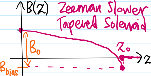
Problem #\(5\): If the atomic beam emerging from the oven along with the counterpropagating laser are oriented along some “\(z\)-axis”, write down the magnetic field \(\mathbf B(z)=B(z)\hat{\textbf k}\) required to make a Zeeman slower.
Solution #\(5\): Assuming one is working at relatively low magnetic field strengths, the low-field basis which diagonalizes the perturbative hyperfine Hamiltonian \(\Delta H_{\text{HFS}}\propto\textbf I\cdot\mathbf J\) is \(|f,m_f\rangle\). In this basis, the expectation of the perturbative Zeeman Hamiltonian \(\Delta H_{\text{Zeeman}}\) is approximately:
\[\langle f,m_f|\Delta H_{\text{Zeeman}}|f,m_f\rangle=g_f\mu_BB(z)m_f\hbar\]
Thus, if one is exploiting an electric dipole transition from a “ground state” \(|fm_f\rangle\) to an “excited state” \(|f’m’_f\rangle\), then one requires the difference in the Zeeman shifts experienced by these \(2\) levels to precisely compensate for the Doppler detuning \(\delta_D=\omega+kv-\omega_{01}\):
\[(g_{f’}m’_f-g_fm_f)\frac{\mu_BB(z)}{\hbar}=\delta_D\]
In practice, one would like to achieve a constant deceleration \(a>0\) so that \(v^2=v_0^2-2az\). This requires a magnetic field from e.g. a tapered solenoid of the form:
\[B(z)=B_0\sqrt{1-\frac{z}{z_0}}+B_{\text{bias}}\]
where \(z_0:=v_0^2/2a\) is the stopping distance, \(B_0:=\frac{\hbar kv_0}{\mu_B(g_{f’}m’_f-g_fm_f)}\) can be interpreted as \(B_0=B(0)-B(z_0)\), and the bias field is \(B_{\text{bias}}=\frac{\hbar(\omega-\omega_{01})}{\mu_B(g_{f’}m’_f-g_fm_f)}\); or at least, if one wishes to completely stop the atoms at \(z=z_0\) (if not, then one may need to experimentally lower \(B_{\text{bias}}\) until one obtains a desired terminal velocity; in that case one should then discontinuously turn off the magnetic field \(B(z):=0\) for \(z>z_0\) so that the E\(1\) transition would again be substantially detuned from resonance and so experience a negligible scattering force \(F_{\gamma}\) after the atoms exit the Zeeman slower).
Problem #\(6\): For the specific case of say sodium atoms \(\text{Na}\) (analogous remarks apply to any alkali atom), explain why electric dipole transitions between the stretched states \(|fm_f\rangle=|22\rangle\) in \(3s_{1/2}\) and \(|f’m’_f\rangle=|33\rangle\) in \(3p_{3/2}\) are a good choice for laser cooling via the scattering force \(F_{\gamma}\)? In this case, what should be the corresponding value of \(B_0\) used in a Zeeman slower (the transition has \(\lambda_{01}=589\text{ nm}\))? What should be the polarization of the incident laser light?
Solution #\(6\): This E\(1\) transition is not only allowed but also forms a closed cycle thanks to the usual E\(1\) selection rules, ensuring no optical pumping into dark states that would prevent a given atom from experiencing any further scattering. One can check that \(B_0\approx 0.12\text{ T}=1200\text{ G}\) is reasonable to achieve in the lab. The incident photons should be \(\sigma^+\) circularly-polarized along the quantization axis \(\hat{\textbf k}\) defined by the \(\textbf B\)-field along which the atomic beam is also propagating.
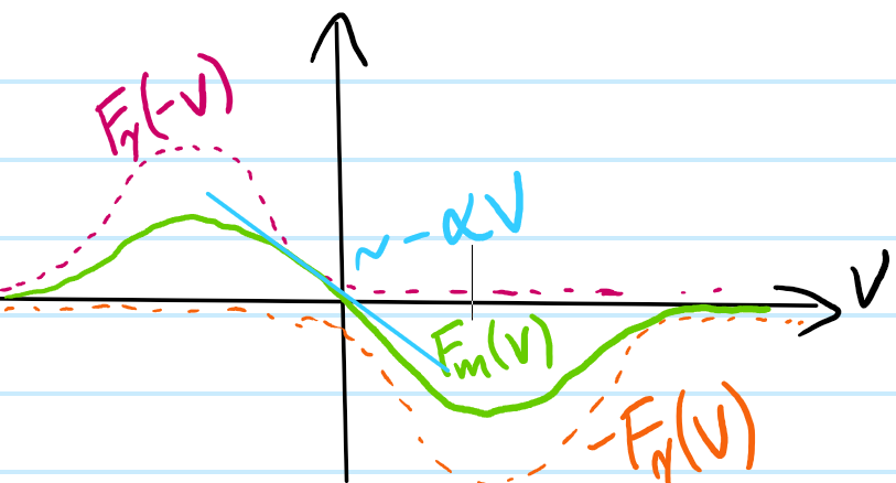
Problem #\(7\): Show, stating any assumptions made, that the velocity-dependent optical molasses force \(F_m(v)\approx -\alpha v\) along an arbitrary axis looks like linear damping with some damping coefficient \(\alpha>0\) for an appropriately-chosen laser detuning \(\delta\). Hence, show that the atom’s kinetic energy \(T(t)=T(0)e^{-t/\tau}\) (supposedly) decays exponentially with time constant \(\tau=m/2\alpha\).
Solution #\(7\): Along any of the \(3\) Cartesian axies, the component of the optical molasses force \(F_m(v)\) along that axis is a superposition of two opposite (but not necessarily equal) scattering forces:
\[F_m(v)=-F_{\gamma}(v)+F_{\gamma}(-v)\approx -2v\frac{\partial F_{\gamma}}{\partial v}(v=0)\]
where the low-velocity assumption \(kv/\Gamma\ll 1\) has been made. This shows that the damping coefficient is:
\[\alpha=2\frac{\partial F_{\gamma}}{\partial v}(v=0)=-4\hbar k^2s\frac{2\delta/\Gamma}{(1+s+(2\delta/\Gamma)^2)^2}\]
So in order for \(\alpha>0\) to actually be damping, one requires \(\delta<0\) to be red-detuned as suggested in the picture. It turns out that in order to treat the two laser beams independently (as has been implicitly done above), they both have the same low \(s\ll 1\) so that neither one saturates the E\(1\) transition too much. In this simple model of optical molasses, one should therefore really take:
\[\alpha=2\frac{\partial F_{\gamma}}{\partial v}(v=0)=-4\hbar k^2s\frac{2\delta/\Gamma}{(1+(2\delta/\Gamma)^2)^2}\]
In some sense, the fact that it looks like linear damping near \(v=0\) is not really conceptually any different from the fact that e.g. systems looks like simple harmonic oscillators near stable equilibria; it’s just taking the \(1\)-st order term in a Taylor series in \(v\).
Kinetic energy is lost through the dissipative power of the molasses force:
\[\dot T=F_m(v)v=-\alpha v^2=-\frac{2\alpha}{m}T\Rightarrow T(t)=T(0)e^{-t/\tau}\]
where \(\tau=m/2\alpha\) is usually on the order of microseconds. This suggests that there is no cooling limit, i.e. that one can quickly cool down arbitrarily close to \(T\to 0\), but this turns out to be impossible, see Problem #\(9\).
Problem #\(8\): For a random walk \(\textbf X_1,\textbf X_2,…,\textbf X_N\) of \(N\) steps, each of identical length \(L=|\textbf X_1|=|\textbf X_2|=…=|\textbf X_N|\), what is the expectation of the total displacement squared \(\langle|\textbf X_1+\textbf X_2+…+\textbf X_N|^2\rangle\)?
Solution #\(8\): All the dot products vanish so:
\[\langle|\textbf X_1+\textbf X_2+…+\textbf X_N|^2\rangle=NL^2\]
Problem #\(9\): Conceptually, what is the issue with the approach taken in Solution #\(7\)? Upon amending it, show that there is actually a Doppler cooling limit, namely a minimum temperature \(T_D\) that can be achieved using the optical molasses technique, given by:
\[k_BT_D=\frac{\hbar\Gamma}{2}\]
Solution #\(9\): The issue with Solution #\(7\) is that, while it accounts for the momentum kick given to the atom during stimulated absorption of photons and also recognizes that spontaneous emission averages to no momentum kick, it neglects fluctuations in both the number of photons absorbed and in the number of photons scattered. Using the result of Problem #\(8\), except here conceptually it’s not a random walk in real space but rather in momentum space with \(\langle p_z^2\rangle(t)=2(\hbar k)^2(2\gamma)t\), the kinetic energy \(T_z\) of an atom in the optical molasses now evolves as (see Foote textbook for the detailed arguments, some sketchy assumptions involved too, and turns out ultimately wrong, see Problem #\(10\)):
\[\dot T_z=-\frac{2\alpha}{m} T_z+\left(1+3\times\frac{1}{3}\right)\frac{\hbar^2k^2}{2m}(2\gamma)\]
So in the steady state \(\dot T_z=0\) and using equipartition \(T_z=k_BT/2\), one finds that:
\[k_BT=-\frac{\hbar\Gamma}{4}\frac{1+(2\delta/\Gamma)^2}{2\delta/\Gamma}\]
is minimized for red-detuned \(\delta<0\) at \(2\delta/\Gamma=-1\), yielding the Doppler cooling limit \(k_BT_D=\hbar\Gamma/2\) as claimed.
Problem #\(10\): Explain why, even after accounting for Poissonian fluctuations in the stimulated absorption and spontaneous emission of photons, the Doppler cooling limit for the optical molasses technique above rests on a “spherical cows in vacuum” foundation.
Solution #\(10\): Simply put, the assumption of a \(2\)-level atom has been implicitly lurking in the discussion the whole time, but it turns out that if one leverages the existence of other sublevels, one can do even better than the Doppler cooling limit above would suggest. Note also that the optical molasses laser cooling technique only provides confinement in \(\textbf k\)-space, but not so much in \(\textbf x\)-space which is also relevant; in other words, laser trapping is to \(\textbf x\) what laser cooling is to \(\textbf k\).
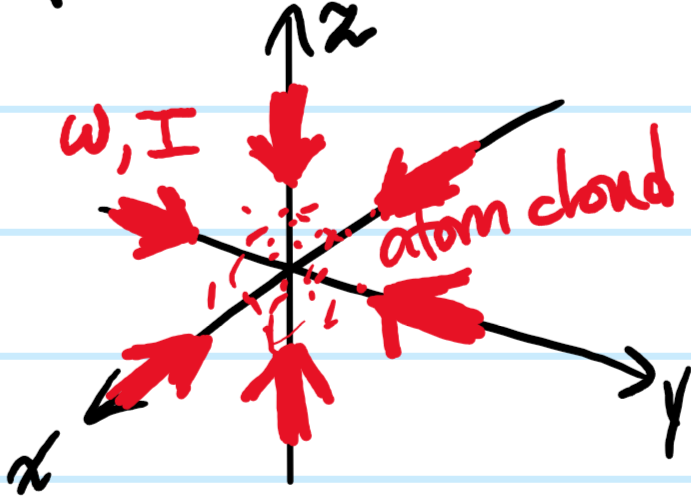
Problem #\(11\): In light of Problem #\(10\), draw \(3\) pictures that summarize how a magneto-optical trap (MOT) works. In particular, it should be clear that the MOT could not work with just a \(2\)-level atom. Also write down explicitly a formula for the MOT force \(F_{\text{MOT}}(z,v)\).
Solution #\(11\):

The MOT force \(F_{\text{MOT}}(z,v)\) is conceptually identical to the optical molasses force \(F_m(v)\) only now the detuning includes not only the \(v\)-dependent Doppler shift but also the \(z\)-dependent Zeeman shift (more precisely, the formula \(F_{\text{MOT}}(z,v)\) that will be given below is the component of the net MOT force \(\textbf F_{\text{MOT}}(\textbf x,\textbf v)\) along the quantization \(z\)-axis of the quadrupolar anti-Helmholtz MOT \(\textbf B\)-field near the origin \(\textbf x\approx\textbf 0\) whose purpose is to generate a nearly uniform magnetic field gradient; a similar equation holds in the \(\rho\)-direction except one should note from \(\frac{\partial}{\partial\textbf x}\cdot\textbf B=0\) that \(\frac{\partial B_{\rho}}{\partial\rho}=-\frac{1}{2}\frac{\partial B_z}{\partial z}\)).
\[F_{\text{MOT}}(z,v)=F_{\gamma}\left(\delta=\omega-kv-\left(\omega_{01}+\frac{g’_f\mu_B}{\hbar}\frac{\partial B_z}{\partial z}z\right)\right)-F_{\gamma}\left(\delta=\omega+kv-\left(\omega_{01}-\frac{g’_f\mu_B}{\hbar}\frac{\partial B_z}{\partial z}z\right)\right)\]
Making the same low Doppler shift assumption \(kv\ll\Gamma\) but now also a low Zeeman shift assumption \(\frac{g’_f\mu_B}{\hbar}\frac{\partial B_z}{\partial z}z\ll\Gamma\), one can check that this reduces to the previous linear damping force of the optical molasses together with a Hookean spring force:
\[F_{\text{MOT}}(z,v)=-\alpha v-\beta z\]
where the spring constant is \(\beta=\frac{\alpha g’_f\mu_B}{\hbar k}\frac{\partial B_z}{\partial z}\) and the damping coefficient \(\alpha\) is as before in Problem #\(7\). Usually, the atom will be overdamped (as is desirable) \(\alpha^2>4\beta m\).
Problem #\(12\): State one advantage and one disadvantage of a MOT compared with just the optical molasses technique.
Solution #\(12\): The advantage of a MOT is that its capture velocity \(v_{c,\text{MOT}}\gg v_{c,m}\) is much greater than that of optical molasses so it is a better trapper, hence its name (indeed, one can load a MOT simply by firing a room-\(T\) vapor, or to get more atoms one can first Zeeman slow them). The disadvantage is that it is not as good of a laser cooler; optical molasses is able to reach much colder temperatures, surpassing the naive Doppler cooling limit \(k_BT_D=\hbar\Gamma/2\) mentioned earlier (this is because of various sub-Doppler cooling mechanisms, notably Sisyphus cooling, that are elaborated upon in the next problem; all that matters for now is that such sub-Doppler cooling mechanisms are effectively disabled when the Zeeman shift exceeds the light shift as in a MOT).
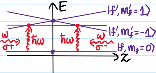
Problem #\(13\): In a MOT, where does the trapping come from?
Solution #\(13\): It does not come from the quadrupolar \(\textbf B\)-field, but rather
Problem #\(14\): Draw a picture to explain how Sisyphus cooling allows. What is the new cooling limit?
Problem #\(15\): Show that the magnetic field strength \(|\textbf B(\textbf x)|\) in free space can never have a strict local maximum provided \(\dot{\textbf E}=\textbf 0\) (this is one version of Earnshaw’s theorem).
Solution #\(15\): One has the usual identity:
\[\frac{\partial}{\partial\textbf x}\times\left(\frac{\partial}{\partial\textbf x}\times\textbf B\right)=\frac{\partial}{\partial\textbf x}\left(\frac{\partial}{\partial\textbf x}\cdot\textbf B\right)-\left|\frac{\partial}{\partial\textbf x}\right|^2\textbf B\]
But thanks to the assumptions of the problem the term on the left vanishes, and in addition to the absence of magnetic monopoles, one concludes that \(\left|\frac{\partial}{\partial\textbf x}\right|^2\textbf B=\textbf 0\).
Now, \(|\textbf B(\textbf x)|\) satisfies the claim if and only if \(|\textbf B(\textbf x)|^2\) satisfies it. In turn, one just has to check that the Hessian \(\frac{\partial^2|\textbf B|^2}{\partial\textbf x^2}\) does not have \(3\) negative eigenvalues anywhere. A sufficient (but not necessary) condition for this would be if \(\text{Tr}\frac{\partial^2|\textbf B|^2}{\partial\textbf x^2}\geq 0\) everywhere. But the trace of the Hessian is just the Laplacian of the original scalar field:
\[\text{Tr}\frac{\partial^2|\textbf B|^2}{\partial\textbf x^2}=\left|\frac{\partial}{\partial\textbf x}\right|^2|\textbf B|^2=2\left|\frac{\partial|\textbf B|}{\partial\textbf x}\right|^2+2|\textbf B|\left|\frac{\partial}{\partial\textbf x}\right|^2\textbf B=2\left|\frac{\partial|\textbf B|}{\partial\textbf x}\right|^2\geq 0\]
which completes the proof.
Problem #\(16\): What is the high-level mechanism of magnetic trapping? What are the \(3\) most common kinds of magnetic traps? (just draw a picture of each one with some annotations, no need for long explanations)
Solution #\(16\): Just as in the Stern-Gerlach experiment, magnetic dipoles in non-uniform magnetic fields experience a force that pushes them towards weaker or stronger magnetic field depending on their orientation relative to the magnetic field. The difference is that in the Stern-Gerlach experiment the atoms are flying in at hundreds of meters/second and getting deflected, way beyond capture velocity, whereas in magnetic trapping they have already been laser cooled. The diThe \(3\) most common magnetic traps are the quadrupole trap (made from a pair of anti-Helmholtz coils as in a MOT), a time-averaged orbiting potential (TOP) trap, and an Ioffe-Pritchard trap, the last of which is the most common and simply consists of \(4\) long cylindrical bars (which form a “linear quadrupole” in direct analogy with an electrostatic quadrupole) and \(2\) Helmholtz-like coils. Key words: radial/\(\rho\)-trapping and axial/\(z\)-trapping. Due to the result of Problem #\(14\), it follows that one can only trap atoms in low-field seeking states (such atoms are called low-field seekers).
Good overview here: https://arxiv.org/pdf/1310.6054