
The purpose of this post is to demonstrate how the scattering operator \(S:\mathcal H_{\text{incident}}^{\infty}\to\mathcal H_{\text{scattered}}^{\infty}\), also called the \(S\)-operator for short, despite being defined to enact the scattering \(|\psi’_{\infty}\rangle=S|\psi_{\infty}\rangle\) of asymptotic incident waves \(|\psi_{\infty}\rangle\) off a potential \(V\) into asymptotic scattered waves \(|\psi’_{\infty}\rangle\), also encodes information about non-scattering states (e.g. bound states and resonant states) of the very same Hamiltonian \(H=T+V\) from which one is scattering quantum particles off of.
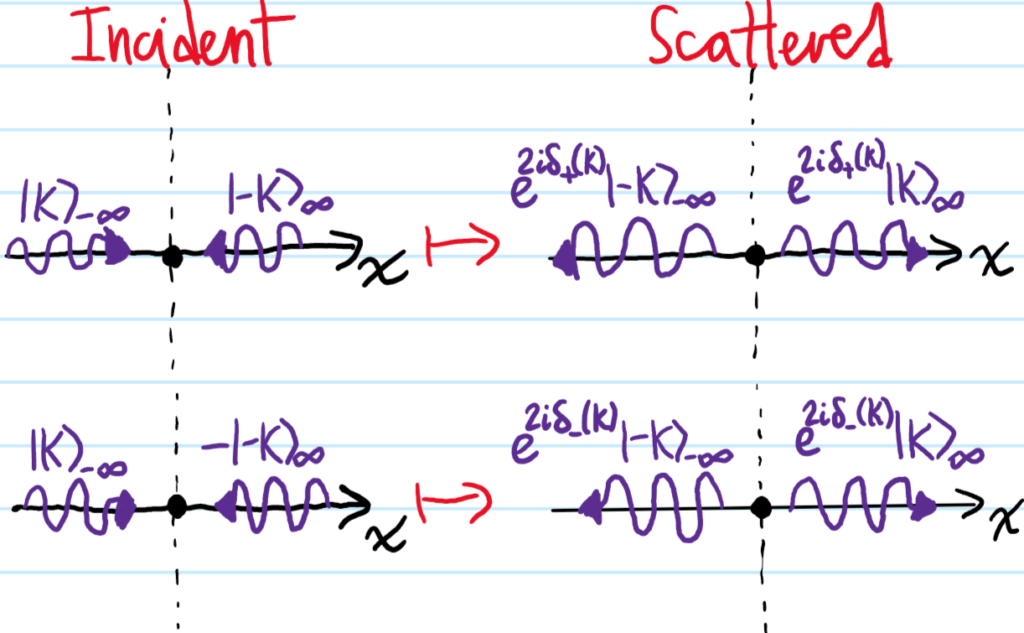
To illustrate this, recall that in one-dimension we have \(4\) distinct asymptotic waves \(|\pm k\rangle_{\pm’\infty}\), defined by the position space wavefunctions \(\langle x|\pm k\rangle_{\pm’\infty}:=e^{\pm ikx}[x\to\pm’\infty]\). We demand that the \(2\) incident waves (from the left and right) individually scatter as \(|k\rangle_{-\infty}\mapsto S|k\rangle_{-\infty}=r_{\rightarrow}|-k\rangle_{-\infty}+t_{\rightarrow}|k\rangle_{\infty}\) and \(|-k\rangle_{\infty}\mapsto S|-k\rangle_{\infty}=t_{\leftarrow}|-k\rangle_{-\infty}+r_{\leftarrow}|k\rangle_{\infty}\) as the picture below shows:

Therefore, with respect to the basis \(|k\rangle_{-\infty},|-k\rangle_{\infty}\) for the space of incident/ingoing waves \(\mathcal H_{\text{incident}}^{\infty}\) and the basis \(|-k\rangle_{-\infty},|k\rangle_{\infty}\) for the space of scattered/outgoing waves\(\mathcal H_{\text{scattered}}^{\infty}\), the matrix representation of \(S\), called the \(S\)-matrix, looks like:
\[[S]_{|k\rangle_{-\infty},|-k\rangle_{\infty}}^{|-k\rangle_{-\infty},|k\rangle_{\infty}}=\begin{pmatrix}r_{\rightarrow}&t_{\leftarrow}\\t_{\rightarrow}&r_{\leftarrow}\end{pmatrix}\]
Recall that we have some unintuitive results on 1D scattering, namely \(t_{\leftarrow}=t_{\rightarrow}:=t\) (not to be confused with time!) and \(r_{\rightarrow}t^*+r_{\leftarrow}^*t=0\). This just says that the columns (equivalently the rows) of the \(S\)-matrix are complex-orthogonal to each other. The orthogonality condition also gives that \(|r_{\leftarrow}|=|r_{\rightarrow}|\), hence by matching asymptotic probability currents \(J_{-\infty}=J_{\infty}\) one obtains \(|r_{\leftarrow}|^2+|t|^2=|r_{\leftarrow}|^2+|t|^2=1\). This discussion proves that \([S]_{|k\rangle_{-\infty},|-k\rangle_{\infty}}^{|-k\rangle_{-\infty},|k\rangle_{\infty}}\in U(2)\) has spectrum \(\Lambda_S\subseteq U(1)\) with complex-orthogonal eigenvectors. One can write such eigenvalues in terms of two real-valued phase shifts \(\delta_{\pm}=\delta_{\pm}(k)\) dependent on the incident momentum \(k\) of the beam of particles, i.e. \(e^{2i\delta_{\pm}}=\frac{r_{\leftarrow}+r_{\rightarrow}}{2}\pm\sqrt{\left(\frac{r_{\leftarrow}-r_{\rightarrow}}{2}\right)^2+t^2}\) with respective eigenvectors that I won’t bother writing down yet.
At this point, to simplify life we will work with an even potential \(V(-x)=V(x)\) so that \(r_{\leftarrow}=r_{\rightarrow}:=r\) coincide. Then the \(S\)-matrix becomes a \(2\times 2\) circulant matrix so we can immediately write down its normalized eigenvectors (this is why I didn’t bother writing them down yet above!) as the two Fourier modes \((1/\sqrt{2},\pm 1/\sqrt{2})^T\). The corresponding eigenvalues of the \(S\)-matrix are straightforwardly \(e^{2i\delta_{\pm}}=r\pm t\), either from the earlier formula or by acting on those Fourier mode eigenvectors (recall that for \(t\in\textbf C\) we have the usual two branches for the square root \(\sqrt{t^2}=\pm t\)). Put another way, the \(S\)-operator is diagonalized in this basis:
\[[S]_{|k\rangle_{-\infty}+|-k\rangle_{\infty}, |k\rangle_{-\infty}-|-k\rangle_{\infty}}^{|-k\rangle_{-\infty}+|k\rangle_{\infty}, |-k\rangle_{-\infty}-|k\rangle_{\infty}}=e^{2i\text{diag}(\delta_+,\delta_-)}\]
Intuitively, if one views \(r,t\in\textbf C\cong\textbf R^2\) as vectors in the complex plane, then for a symmetric potential they must be \(\textbf R^2\)-orthogonal to each other, consistent with their \(\textbf C^2\)-orthogonality \(rt^*+(rt^*)^*=2\Re(rt^*)=0\Rightarrow |r\pm t|^2=|r|^2\pm 2\Re(rt^*)+|t|^2=|r|^2+|t|^2=1\) so that \(r\pm t=e^{2i\delta_{\pm}}\in U(1)\) as claimed all along:

In hindsight, it’s actually not too surprising why the eigenstates of the \(S\)-operator were given by the Fourier modes \(|k\rangle_{-\infty}\pm|-k\rangle_{\infty}\) when \(V(-x)=V(x)\). Physically, these look like simultaneously throwing in two identical beams of particles from both the left and right, just that one setup has even parity while the other setup has odd parity. After all, because \([H,\Pi]=0\) conserves parity, the interaction of the particles with \(H\) (in other words the scattering!) has to preserve parity asymptotically in the past and future. And those particular linear combinations are essentially the only way to construct \(\Pi\)-eigenstates out of the incident waves \(|k\rangle_{-\infty},|-k\rangle_{\infty}\) which don’t have definite parity.
Example: So far we’ve gotten away with proving several general results on one-dimensional scattering, assuming only a symmetric potential \(V(-x)=V(x)\). However, to actually compute \(S\)-matrices (regardless of which basis of scattering states you want to work in) we ultimately have to say what \(V(x)\) we’re talking about! To that effect, consider our favorite finite potential well of width \(L>0\) and depth \(V_0>0\). The goal is to compute the phase shifts \(\delta_{\pm}(k)\) that completely characterize all scattering phenomena off this potential. If we define \(|\psi_{\text{well}}^{\pm}\rangle:=\alpha_{\pm}(|k’\rangle_{[-L/2,L/2]}\pm|-k’\rangle_{[-L/2,L/2]})\) to be the compactly supported even/odd state in the finite potential well region, with increased momentum \(k’=\sqrt{2m(E+V_0)}/\hbar>k=\sqrt{2mE}/\hbar\), then the even/odd-parity total states \(|\psi_{\pm}\rangle\) are given by the superpositions \(|\psi_{\pm}\rangle=|k\rangle_{-\infty}\pm|-k\rangle_{\infty}+e^{2i\delta_{\pm}(k)}(|-k\rangle_{-\infty}\pm|k\rangle_{\infty})+|\psi_{\text{well}}^{\pm}\rangle\). Now because \(\langle x|\psi_{\pm}\rangle\) and \(\langle x|K|\psi_{\pm}\rangle\) should both be continuous at \(x=L/2\) (and by parity also at \(x=-L/2\)), it follows that \(\langle x|K\ln|\psi_{\pm}\rangle\) also needs to be continuous at \(x=\pm L/2\). Approaching \(x=L/2\) from the left means:
\[\langle L/2|K\ln|\psi_{\pm}\rangle=k’\frac{\langle L/2|k’\rangle\mp\langle L/2|-k’\rangle}{\langle L/2|k’\rangle\pm\langle L/2|-k’\rangle}\]
Whereas approaching \(x=L/2\) from the right means:
\[\langle L/2|K\ln|\psi_{\pm}\rangle=k\frac{\mp\langle L/2|-k\rangle\pm e^{2i\delta_{\pm}(k)}\langle L/2|k\rangle}{\pm\langle L/2|-k\rangle\pm e^{2i\delta_{\pm}(k)}\langle L/2|k\rangle}\]
Treating it as a Mobius transformation, one can isolate for the \(S\)-operator eigenvalues:
\[e^{2i\delta_{\pm}(k)}=\frac{(k+k’\frac{\langle L/2|k’\rangle\mp\langle L/2|-k’\rangle}{\langle L/2|k’\rangle\pm\langle L/2|-k’\rangle})(k-k\frac{\mp\langle L/2|-k\rangle\pm\langle L/2|k\rangle}{\pm\langle L/2|-k\rangle\pm\langle L/2|k\rangle})}{(k-k’\frac{\langle L/2|k’\rangle\mp\langle L/2|-k’\rangle}{\langle L/2|k’\rangle\pm\langle L/2|-k’\rangle})(k+k\frac{\mp\langle L/2|-k\rangle\pm \langle L/2|k\rangle}{\pm\langle L/2|-k\rangle\pm \langle L/2|k\rangle})}\]
These simplify respectively to:
\[e^{2i\delta_{+}(k)}=-e^{-ikL}\frac{k’\tan(k’L/2)-ik}{k’\tan(k’L/2)+ik}\]
\[e^{2i\delta_{-}(k)}=e^{-ikL}\frac{k\tan(k’L/2)-ik’}{k\tan(k’L/2)+ik’}\]
Hence we can read off the phase shifts:
\[\delta_{+}(k)=-\frac{kL}{2}-\arctan\left(\frac{k}{k’}\cot\frac{k’L}{2}\right)\]
\[\delta_-(k)=-\frac{kL}{2}-\arctan\left(\frac{k’}{k}\cot\frac{k’L}{2}\right)\]
where \(k’=k'(k)\) through the energy \(E=\frac{\hbar^2k^2}{2m}=\frac{\hbar^2k’^2}{2m}-V_0\). The phase shift difference is obtained either by dividing the original exponentials or applying the arctan subtraction identity:
\[\delta_+(k)-\delta_-(k)=\text{arctan}\left(\frac{k’^2-k^2}{2kk’}\sin k’L\right)\]
Finally, although the eigenvalues \(e^{2i\delta_{\pm}(k)}\) of the \(S\)-operator lie in \(U(1)\) when \(k\in\textbf R\), if we instead allow \(k\in\textbf C\) to roam the entire complex momentum plane, then the exponential \(e^{2i\delta_{\pm}(k)}\) is no longer restricted to lie in \(U(1)\). In particular, focus for a moment on just letting \(k\in i\textbf R\subseteq\textbf C\) roam the imaginary axis. We know from experience that the \(E<0\) bound state wavefunctions of the finite potential well (of which one even-parity bound ground state always exists) look like the pure harmonics of the infinite potential well but with an exponential leakage \(\propto e^{\pm \kappa x}[x\to\mp \infty]\) into the classically forbidden regions. These real exponentials \(e^{\pm\kappa x}\) are clearly very similar-looking to the complex exponentials \(e^{\pm ikx}\) that the scattering state wavefunctions involve. This is therefore how I would motivate this trick of looking at \(k=i\kappa’\) for \(\kappa’\in\textbf R\). We also know that the bound states of the finite potential well have to have definite parity (unlike the scattering states) so it seems plausible that maybe these bound states can emerge from our scattering states \(|\psi_{\pm}\rangle\) constructed earlier that do happen to have definite parity \(\pm\) as well. Therefore, with the substitution \(k=i\kappa’\), the total even/odd-parity scattering states \(|\psi_{\pm}\rangle\) transform asymptotically into looking like:
\[\langle x|\psi_{\pm}\rangle= (e^{-\kappa’ x}+e^{2i\delta_{\pm}(i\kappa’)}e^{\kappa’ x})[x\to-\infty]\pm(e^{\kappa’ x}+e^{2i\delta_{\pm}(i\kappa’)}e^{-\kappa’ x})[x\to\infty]\]
But clearly these candidate bound states \(|\psi_{\pm}\rangle\) (whether even or odd) can only have a hope of being normalizable (as required for bound states but not scattering states!) iff \(\kappa'<0\). Therefore, define \(\kappa:=-\kappa’>0\):
\[\langle x|\psi_{\pm}\rangle= (e^{\kappa x}+e^{2i\delta_{\pm}(-i\kappa)}e^{-\kappa x})[x\to-\infty]\pm(e^{-\kappa x}+e^{2i\delta_{\pm}(-i\kappa)}e^{\kappa x})[x\to\infty]\]
In order to kill the non-normalizable exponentials, we must therefore find values of \(k=-i\kappa\) on the lower imaginary axis such that the \(S\)-operator eigenvalues vanish \(e^{2i\delta_{\pm}(k)}=0\). More precisely, if we want to realize our dream of \(|\psi_+\rangle\) being an even parity bound state, then we need:
\[e^{2i\delta_+(-i\kappa)}=-e^{-\kappa L}\frac{k’\tan(k’L/2)-\kappa}{k’\tan(k’L/2)+\kappa}=0\]
where now \(\kappa^2+k’^2=2mV_0/\hbar^2\) are constrained to lie on a circle \(k’-i\kappa\in \sqrt{2mV_0}/\hbar U(1)\) in the complex momentum plane \(\textbf C\). Meanwhile the condition above is satisfied iff the numerator vanishes \(\kappa=k’\tan(k’L/2)\).
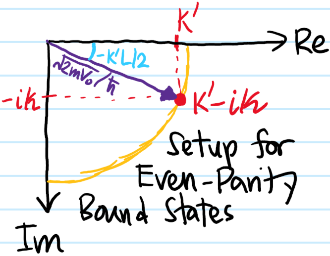
This is the usual transcendental system of simultaneous equations for \((\kappa,k’)\in (0,\infty)^2\) that need to be solved to find even-parity bound states of the finite potential well. Graphically, it is clear that there always exists at least one ground state solution with possibly more depending on the width \(L\) and depth \(V_0\) of the potential.
For odd-parity bound states, we require \(e^{2i\delta_-(-i\kappa)}=0\) which instead leads to \(k’=-\kappa\tan k’L/2\). Graphically, this is a mirroring of the setup for even-parity states about the \(\Im =-\Re \) diagonal.
Resonances in Particle Physics
Recall from classical physics that the \(n\)-th harmonic for \(n\in\textbf Z^+\) on say a violin string of length \(L\) or inside a pipe of length \(L\) with nodes at both ends has wavelength \(\lambda=\lambda_n\) quantized according to \(n\lambda=2L\). Loosely, one might say that such harmonics “maximize transmission” of the instrument’s pleasant sound. It turns out the same principle is true when it comes to scattering quantum particles off a finite potential well of length \(L\); if the de Broglie wavelength \(\lambda=2\pi/k\) satisfies \(n\lambda=2L\), then the transmission probability is maximized \(T=|t|^2=|(e^{2i\delta_+(k)}-e^{2i\delta_-(k)})/2|^2=\sin^2(\delta_+(k)-\delta_-(k))=1\rightarrow \delta_+-\delta_-\equiv \pi/2\pmod \pi\) (alternatively, from the earlier geometric picture it is clear that \(|t|=\sin|\delta_+(k)-\delta_-(k)|\)). Equivalently, if one scatters in quantum particles exactly with energy \(E=\frac{n^2\pi^2\hbar^2}{2mL^2}+V_0\) for some \(n\in\textbf Z^+\), then the particle is guaranteed to transmit through with no reflection \(R=|r|^2=0\). Note that these energies are precisely those of the bound states in an infinite potential well with the bottom of the well raised to \(V_0\) (I’m not sure if this is a coincidence or something more universal about de Broglie quantization). This is one form of resonance in quantum mechanical scattering experiments, which one can think of as transmission resonances.

However, there is another sense of the word “resonance” as used in particle physics which is related to the above discussion. Specifically, a resonant state of a quantum system is one which is metastable, i.e. unstable in the long run \(t\to\infty\). Resonant states are thus a kind of hybrid of a bound state and a scattering state. What kind of quantum system admits resonant states? The finite potential well, it turns out, doesn’t. Instead, when asked to think about a potential \(V(x)\) admitting a resonant state, one’s gut reaction should be to visualize a trapping environment such as:
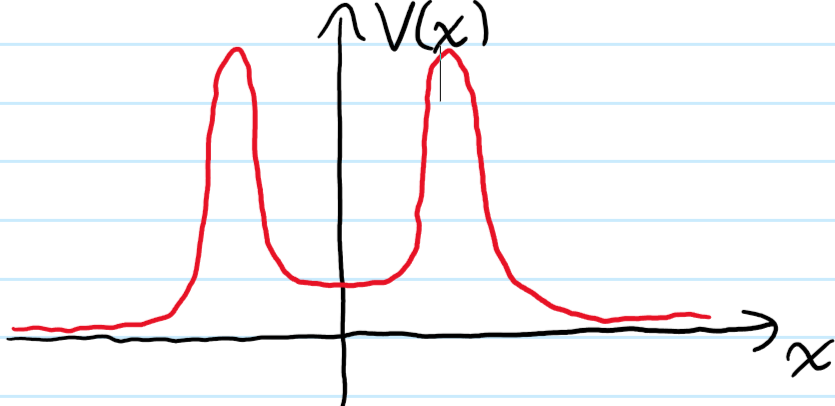
Here, the intuition is that there are no bound (i.e. permanently stable) states because the particle can quantum tunnel through the walls of the trap (don’t call it a well anymore!). Hence, the next best thing you can get is a resonant state.
We can idealize the above picture by considering a double Dirac delta potential trap \(V(x)=V_0L(\delta(x-L/2)+\delta(x+L/2))\) of width \(L>0\) and height \(V_0>0\) (the factor of \(L\) is needed to compensate the fact that delta functions always have the inverse dimension of their argument. This ensures \(V_0\) has units of energy). Integrating the Schrodinger equation in an \(\varepsilon\)-ball around the spike at \(x=L/2\) yields the magnitude of the first derivative’s discontinuity \(\psi'(L/2)^+-\psi'(L/2)^-=\frac{2mV_0 L}{\hbar^2}\psi(L/2)\) where the quantity \(\psi(L/2)\) is well-defined because \(\psi(x)\) itself will be continuous at \(x=L/2\) (and indeed, is the other condition we need to patch). Since this potential is again even \(V(-x)=V(x)\), we should scatter in particles from the left and right simultaneously and patch only at \(x=L/2\); looking at the even-parity scattering state for now (odd case is similar):
\[\alpha(e^{ikL/2}+e^{-ikL/2})=e^{-ikL/2}+e^{2i\delta_+(k)+ikL/2}\]
\[-ike^{-ikL/2}+ike^{2i\delta_+(k)+ikL/2}-ik\alpha(e^{ikL/2}-e^{-ikL/2})=\frac{2mV_0 L}{\hbar^2}\left(e^{-ikL/2}+e^{2i\delta_+(k)+ikL/2}\right)\]
Isolating for the eigenvalue \(e^{2i\delta_+(k)}\) yields:
\[e^{2i\delta_+(k)}=-e^{-ikL}\frac{k\tan(kL/2)-\tilde k-ik}{k\tan(kL/2)-\tilde k+ik}\]
where \(\tilde k:=2mV_0 L/\hbar^2\). Unlike the finite potential well, the Dirac double delta potential trap admits no bound states because there does not exist any \(k\) on the lower imaginary axis such that \(e^{2i\delta_+(k)}=0\). To prove this, write \(k=-i\kappa\) for \(\kappa>0\) so that we need to solve the real equation \(\tanh\frac{\kappa L}{2}=-1-\frac{\tilde k}{\kappa}\). But the range of \(\tanh\) is \((-1,1)\) and for \(\kappa>0\) the right-hand side is always less than \(-1\), hence there can be no solution for \(\kappa>0\) (it turns out there are solutions for \(\kappa<0\) whenever \(\tilde kL\leq\approx 0.5569290855\) where the constant satisfies the transcendental equation \(\tanh\left(\frac{1}{2}+\frac{x}{4}\right)=1-\frac{1}{\frac{1}{x}-\frac{1}{2}}\) but we already saw these were unphysical). Of course, this non-existence of bound states is what we had expected all along. However, there do exist complex momenta \(k\in\textbf C-i\textbf R\) not on the imaginary axis for which the phase eigenvalue \(e^{2i\delta_+(k)}=0\) does vanish. But does that have any associated physical meaning? Well, just like the bound state case \(k=-i\kappa\) led to the negative energy \(E=-\hbar^2\kappa^2/2m\) characteristic of bound states, a general complex momentum \(k=\Re k+i\Im k\) leads to a complex energy \(E=\frac{\hbar^2(\Re^2 k-\Im^2 k)}{2m}+i\frac{\hbar^2}{m}\Re k\Im k\). To see what this means, consider that an \(H\)-eigenstate \(|E\rangle\) with such a complex energy \(E\) would evolve in time as:
\[|E(t)\rangle=e^{-iEt/\hbar}|E(0)\rangle=e^{-i\hbar(\Re^2 k-\Im^2 k)t/2m}e^{\hbar\Re k\Im k t/m}|E(0)\rangle\]
Thus, such an \(H\)-eigenstate \(|E(t)\rangle\) oscillates at angular frequency \(\omega=\hbar(\Re^2 k-\Im^2 k)/2m\). If we assume that \(\Re k\Im k<0\) have opposite signs (i.e. \(k\in\textbf C\) either lives in the second or fourth quadrant), then\(|E(t)\rangle\) also decays (rather than grows) exponentially in amplitude with time constant \(\tau=-m/\hbar\Re k\Im k>0\). This turns out to correspond to a resonant state with \(\tau\) representing the typical time scale for which one can trap the particle before it tunnels away. It is common to define the energy width \(\Gamma:=-2\hbar^2\Re k\Im k/m\) of such a metastable resonant state so that \(\Gamma\tau=2\hbar\) has a Heisenberg form (the reason for this name has to do with the Breit-Wigner distribution in particle physics).
So assuming we’ve found some non-imaginary complex momentum \(k=\Re k+i\Im k\in\textbf C-i\textbf R\) for which the outgoing waves are suppressed \(e^{2i\delta_+(k)}=0\), recall this means that the even parity scattering state (incorporating the time dependence) reduces to looking like \(\langle x|\psi_+(t)\rangle\to e^{-iEt/\hbar+ikx}=e^{i(\Re k x-\hbar(\Re^2k-\Im^2k)t/2m)}e^{-\Im k(x-\hbar\Re k t/m)}\) as \(x\to -\infty\) and \(\langle x|\psi_+(t)\rangle\to e^{-iEt/\hbar-ikx}=e^{-i(\Re k x+\hbar(\Re^2k-\Im^2k)t/2m)}e^{\Im k(x+\hbar\Re k t/m)}\) as \(x\to\infty\). But this simply describes the wavefunction of a particle that has tunneled out of trap, moving away in both directions \(x\to\pm\infty\) from the trap at speed \(v=\hbar|\Re k|/m\). Such a wavefunction \(|\psi_+\rangle\notin L^2(\textbf R\to\textbf C,dx)\) is not normalizable as is typical of resonant states, analogous to scattering states (for instance, despite being an \(H\)-eigenstate, its complex energy eigenvalue \(E\in\textbf C\) violates the supposed Hermiticity of the Hamiltonian \(H\), so such a state \(|\psi_+\rangle\) cannot belong to the state space \(L^2\)).
So then back to the double Dirac delta trap, we expect intuitively it should have an even resonant state, which mathematically means that its \(S\)-operator eigenvalue \(e^{2i\delta_+(k)}=-e^{-ikL}\frac{k\tan(kL/2)-\tilde k-ik}{k\tan(kL/2)-\tilde k+ik}\) should vanish somewhere in quadrant \(2\) or \(4\) of the complex \(k\)-plane. Indeed, this means we expect the numerator to vanish \(k\tan(kL/2)=\tilde k+ik\). One can check that this is equivalent to the requirement \(e^{ikL}=-1-\frac{2ik}{\tilde k}\). If the potential were infinitely trapping so that \(\tilde k\to\infty\), then we would have real momenta \(k=k_n=\frac{\pi}{L}+\frac{2\pi n}{L}\in\textbf R\). These are bound states because an infinitely strong double Dirac delta trap looks like an infinite potential well (at least in the trapping region \(x\in(-L/2,L/2)\); asymptotically all incident waves are reflected at the walls and \(e^{2i\delta_+(k)}=-e^{-ikL}\neq 0\) with the minus sign due to the phase shift of a reflection. Another point is that we previously saw bound states should have \(k\) living in the lower imaginary axis, but here \(k\in\textbf R\). This is a pathological exception to the usual rule since ordinarily for finite \(\tilde k\) we didn’t expect any bound states in the first place but an infinite trapping potential forbids particles from tunneling out, so would-be resonant states transmogrify into bound states in this artificial limit \(\tilde k\to\infty\)). Now suppose that the potential trapping strength \(\tilde k\) is still strong but finite (this is the limit we work in). Focus on the \(n=0\) bound state for which \(k=\pi/L\). It’s position space wavefunction in the trap looks just like the fundamental harmonic on a violin string. We want to know where this initially real \(k=\pi/L\) instead ends up in \(\textbf C\). To first order in \(1/\tilde k\), it simply moves to (going to first-order in the log and using binomial expansion) \(ikL\approx i\pi+2ik/\tilde k\Rightarrow k\approx \frac{\pi}{L}(1+2/\tilde kL)\). However, to second order \(ikL\approx i\pi+2ik/\tilde k+4k^2/\tilde k^2\). We can take the first-order solution for \(k\) and substitute in for the \(k^2\) term, keeping only terms to order \(1/\tilde k^2\), and end up getting \(k\approx\frac{\pi}{L}(1+2/\tilde kL+4/\tilde k^2L^2)-\frac{4\pi^2}{\tilde k^2L^3}i\) neglecting real and imaginary terms of order \(O_{\tilde k\to\infty}(1/\tilde k)^3\). This shows \(k\) moving toward the right and down in the complex momentum plane \(\textbf C\), which is the resonant (ground) state momentum!