
Problem: Deduce the Hamilton-Jacobi equation of classical mechanics.
Solution: Instead of viewing the action \(S=S[\mathbf x(t)]\) as a functional of the particle’s trajectory \(\mathbf x(t)\), it can be viewed more simply as a scalar field \(S(\mathbf x,t)\) in which the initial point in spacetime \((t_0,\mathbf x_0)\) is fixed and one simply takes the on-shell trajectory from \((t_0,\mathbf x_0)\) to \((t,\mathbf x)\). Then the total differential \(dS=\mathbf p\cdot d\mathbf x\) (follows from the usual Noetherian calculation) so in particular:
\[\mathbf p=\frac{\partial S}{\partial\mathbf x}\]
Intuitively, this is saying that the particle moves in a direction (the direction of the momentum \(\mathbf p\)) orthogonal to the contour surfaces of the action field \(S\), i.e. such isosurfaces can be viewed as “wavefronts”. Then the total time derivative is:
\[\dot S=L\]
But \(\frac{\partial S}{\partial t}+\frac{\partial S}{\partial\mathbf x}\cdot\dot{\mathbf x}=\frac{\partial S}{\partial t}+\mathbf p\cdot\dot{\mathbf x}\). Thus, isolating for \(H=\mathbf p\cdot\dot{\mathbf x}-L\) yields the Hamilton-Jacobi nonlinear \(1^{\text{st}}\)-order PDE for \(S(\mathbf x,t)\):
\[-\frac{\partial S}{\partial t}=H\left(\mathbf x,\frac{\partial S}{\partial\mathbf x},t\right)\]
Problem: When \(\partial H/\partial t=0\), the Hamiltonian is conserved with energy \(H=E\), so this motivates the additive separation of variables, \(S(\mathbf x,t):=S_0(\mathbf x)-Et\) for some constant \(E\). What does the Hamilton-Jacobi equation simplify to in this case? For a single non-relativistic particle of mass \(m\) moving in a potential \(V(\mathbf x)\), what does this look like? What about in \(1\) dimension?
Solution: \[H\left(\mathbf x,\frac{\partial S_0}{\partial\mathbf x}\right)=E\]
which for \(H(\mathbf x,\mathbf p)=|\mathbf p|^2/2m+V(\mathbf x)\) looks like:
\[\frac{1}{2m}\biggr|\frac{\partial S_0}{\partial\mathbf x}\biggr|^2+V(\mathbf x)=E\]
and in \(1\) dimension is integrable to the explicit solution:
\[S_0(x)=\pm\int ^xdx’\sqrt{2m(E-V(x’))}\]
In particular, the usual trajectory \(x(t)\) can be obtained by treating \(S_o=S_0(x,t;E)\) as a family of solutions parameterized by the energy \(E\); this works because \(S_0\) can be a viewed as a particular generating function of a canonical transformation \((\mathbf x,\mathbf p,H)\mapsto (\mathbf x’,\mathbf p’,H’)\) in which the “boosted” Hamiltonian vanishes \(H’=0\).
\[\frac{\partial S_0}{\partial E}=-t_0\Rightarrow t-t_0=\pm\sqrt{\frac{m}{2}}\int_{x_0}^{x(t)}\frac{dx’}{\sqrt{E-V(x’)}}\]
Problem: Above, the static field \(S_0(\mathbf x)\) was introduced to simplify the Hamilton-Jacobi equation when the energy \(E\) was conserved. However, if one pulls back to the level of functionals rather than fields, one can define an analogous abbreviated action functional \(S_0[\mathbf x]\) which depends only on the path \(\mathbf x\) taken rather than the trajectory \(\mathbf x(t)\). Define \(S_0[\mathbf x]\), and moreover show that when the energy \(E\) is conserved, the on-shell path is a stationary point of \(S_0\) (this is called Maupertuis’s principle).
Solution: The abbreviated action for a single particle of mass \(m\) and (non-relativistic) energy \(E=|\mathbf p|^2/2m +V(\mathbf x)\) is:
\[S_0[\mathbf x]:=\int d\mathbf x\cdot\mathbf p=\int ds |\mathbf p|=\int ds\sqrt{2m(E-V(\mathbf x))}\]
(modifying this to \(S_0[\mathbf x]:=\int ds |\mathbf p|=\int ds\sqrt{2(E-V(\mathbf x))}\) allows for interpretation as an \(N\)-particle system in configuration space \(\mathbf x\in\mathbf R^{3N}\) with the Riemannian “mass metric” \(ds^2=m_1|d\mathbf x_1|^2+…+m_N|d\mathbf x_N|^2\)).
To find the stationary paths of \(S_0[\mathbf x]\) subject to the constraint \(H(\mathbf x,\mathbf p)=E\), one can implement a Lagrange multiplier \(\gamma(\tau)\) to perform unconstrained extremization of:
\[S[\mathbf x(\tau)]:=S_0[\mathbf x(\tau)]-\int d\tau\gamma(\tau)(H(\mathbf x,\mathbf p)-E)=\int d\tau (\mathbf p\cdot\dot{\mathbf x}-\gamma(\tau)(H(\mathbf x,\mathbf p)-E))\]
The Euler-Lagrange equations lead to Hamilton’s equations:
\[\frac{d\mathbf x}{d\tau}=\gamma\frac{\partial H}{\partial\mathbf p}\]
\[\frac{d\mathbf p}{d\tau}=-\gamma\frac{\partial H}{\partial\mathbf x}\]
provided the Lagrange multiplier \(\gamma=dt/d\tau\) encodes reparameterization invariance; with this choice it’s clear that the integrand in the functional \(S\) was nothing more than the Lagrangian \(L=\mathbf p\cdot\dot{\mathbf x}-H\) (plus an unimportant constant \(E\)) so Maupertuis’s principle reduces to the usual Hamilton’s principle.
Problem: What does Fermat’s principle in ray optics assert? Hence, derive the ray equation.
Solution: The time functional \(T=T[\mathbf x(s)]\) of a ray trajectory \(\mathbf x(s)\) is stationary on-shell. That is:
\[cT[\mathbf x(s)]=\int ds n(\mathbf x(s))\]
This is reparameterization invariant, since one can arbitrarily parameterize \(\mathbf x=\mathbf x(t)\) and replace \(ds=dt|\dot{\mathbf x}|\). The corresponding Euler-Lagrange equations are:
\[\frac{d}{dt}\left(n(\mathbf x)\frac{\dot{\mathbf x}}{|\dot{\mathbf x}|}\right)=|\dot{\mathbf x}|\frac{\partial n}{\partial\mathbf x}\]
But by choosing the natural parameterization \(t:=s\) one has \(|d\mathbf x/ds|=1\), hence the ray equation:
\[\frac{d}{ds}\left(n\frac{d\mathbf x}{ds}\right)=\frac{\partial n}{\partial\mathbf x}\]
This can also be written in terms of the curvature vector \(\boldsymbol{\kappa}=d^2\mathbf x/ds^2\):
\[\boldsymbol{\kappa}=\left(\frac{\partial\ln n}{\partial\mathbf x}\right)_{\perp d\mathbf x}\]
Problem: Starting from an arbitrary Cartesian component \(\psi(\mathbf x,t)=\psi_0(\mathbf x)e^{i(k_0cT(\mathbf x)-\omega t)}\) of either the \(\mathbf E\) or \(\mathbf B\) fields of a light wave (here \(\omega=ck_0\) with \(k_0=2\pi/\lambda_0\) is the free space wavenumber), make the eikonal approximation to the dispersionless wave equation obeyed by \(\psi\) in order to obtain the (scalar) eikonal equation. By defining light rays as the integral curves of the eikonal field \(cT(\mathbf x)\) (a kind of local optical path length), reproduce the vector eikonal equation from Fermat’s principle above.
Solution: The ansatz \(\psi(\mathbf x,t)=\psi_0(\mathbf x)e^{i(k_0cT(\mathbf x)-\omega t)}\) is easy to justify; the \(e^{-i\omega t}\) is a just a Fourier transform factor that reduces the wave equation \(\biggr|\frac{\partial}{\partial\mathbf x}\biggr|^2\psi=\frac{n^2}{c^2}\frac{\partial^2\psi}{\partial t^2}\) to a Helmholtz equation \(\biggr|\frac{\partial}{\partial\mathbf x}\biggr|^2\psi=-n^2k_0^2\psi\). The remaining piece is just a polar parameterization of an arbitrary \(\mathbf C\)-valued spatial field \(\psi_0(\mathbf x)e^{ik_0cT(\mathbf x)}\). One obtains:
\[\biggr|\frac{\partial cT}{\partial\mathbf x}\biggr|^2=n^2+\frac{1}{k_0^2\psi_0}\biggr|\frac{\partial}{\partial\mathbf x}\biggr|^2\psi_0+\frac{2i}{k_0\psi_0}\frac{\partial\psi_0}{\partial\mathbf x}\cdot\frac{\partial cT}{\partial\mathbf x}+\frac{i}{k_0}\biggr|\frac{\partial}{\partial\mathbf x}\biggr|^2cT\]
The eikonal approximation amounts to taking the ray optics limit \(k_0\to\infty\) (in practice, the wavelength \(2\pi/k_0\) has to be much shorter than all other length scales), and yields the (scalar) eikonal equation:
\[\biggr|\frac{\partial cT}{\partial\mathbf x}\biggr|=n\]
A light ray is thus a trajectory \(\mathbf x(s)\) with unit tangent vector:
\[\frac{d\mathbf x}{ds}=\frac{1}{n}\frac{\partial cT}{\partial\mathbf x}\]
The rest is an application of the chain rule:
\[\frac{d}{ds}=\frac{\partial}{\partial\mathbf x}\cdot\frac{d\mathbf x}{ds}=\frac{1}{n}\frac{\partial}{\partial\mathbf x}\cdot\frac{\partial cT}{\partial\mathbf x}\]
followed by the identity:
\[\left(\frac{\partial cT}{\partial\mathbf x}\cdot\frac{\partial}{\partial\mathbf x}\right)\frac{\partial cT}{\partial\mathbf x}=\frac{1}{2}\frac{\partial}{\partial\mathbf x}\biggr|\frac{\partial cT}{\partial\mathbf x}\biggr|^2\]
to deduce the (vector) eikonal equation of motion for ray trajectories just as Fermat’s principle predicts.
Problem: Hence, what is Hamilton’s optics-mechanics analogy?
Solution: In a nutshell, the isomorphism proceeds as:
\[(n(\mathbf x), cT)\leftrightarrow (|\mathbf p(\mathbf x)|,S_0)\]
Problem: Use Hamilton’s optics-mechanics analogy to solve the brachistochrone problem (this was how Johann Bernoulli originally solved it).
Solution: By energy conservation, the speed of the particle at distance \(y>0\) below its initial dropping height is \(v=\sqrt{2gy}\). By Fermat’s principle, minimizing the time functional then amounts to treating the particle as a light ray with \(n(\mathbf x)=c/v(y)\). So the question becomes how do light rays bend in a horizontally stratified medium with \(n(y)\propto y^{-1/2}\)? The answer is given by the ray equations:
\[\frac{d}{ds}\begin{pmatrix} y^{-1/2}dx/ds \\ y^{-1/2}dy/ds\end{pmatrix}=\begin{pmatrix}0 \\ y^{-1/2}/2\end{pmatrix}\]
The horizontal component expresses Snell’s law since \(dx/ds=\sin\theta\) (it expresses momentum conservation along the homogeneous \(\partial n/\partial x=0\) direction). Using the tangent vector constraint \(ds^2=dx^2+dy^2\) gives the ODE of a cycloid:
\[\frac{dy}{dx}=\sqrt{\frac{\text{const}}{y}-1}\]
(the vertical component ODE has an analytical solution \(y(s)=-s^2/8R+s\) which is contained in the cycloid, so is redundant information).
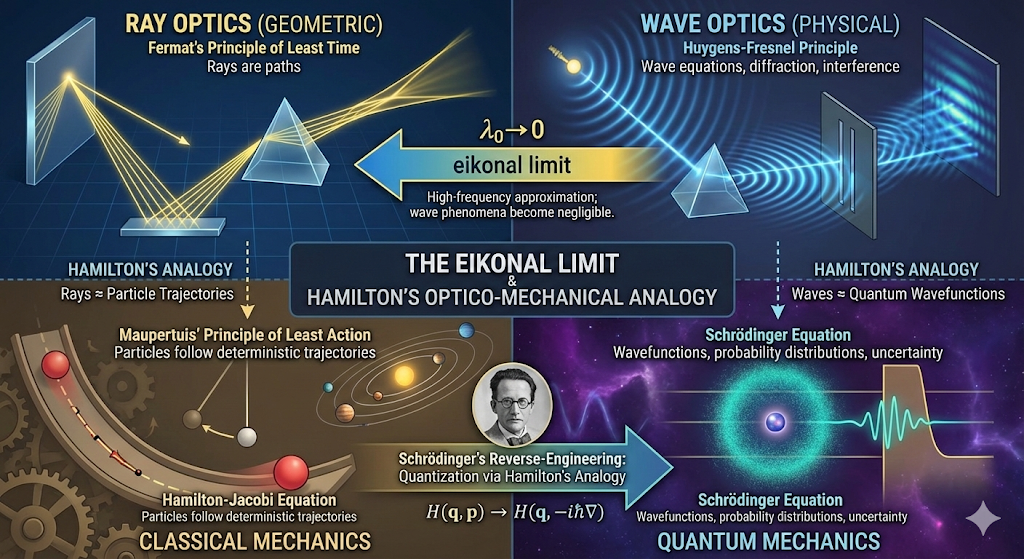
Problem: How did Hamilton’s optics-mechanics analogy inspire Schrodinger to propose his famous equations of quantum mechanics?
Solution: Essentially, Schrodinger asked: ray optics is to wave optics as classical mechanics is to what? In other words, one imagines there exists a wave theory of particles/matter and one would like to take the “inverse eikonal limit” of classical mechanics (here, “inverse eikonal limit” is usually called quantization):
Just as light rays propagate parallel to their phase fronts:
\[\frac{d\mathbf x}{ds}=\frac{1}{n}\frac{\partial cT}{\partial\mathbf x}\]
Particles propagate parallel to their “action fronts” exactly according to Hamilton’s analogy:
\[\frac{d\mathbf x}{ds}=\frac{1}{|\mathbf p(\mathbf x)|}\frac{\partial S_0}{\partial\mathbf x}\]
Already this suggests that the action should have some phase interpretation. More precisely, it should be the phase of the particle’s de Broglie wave in units of \(\hbar\). It’s also not obvious that particle’s should be described by a scalar wave field rather than e.g. the electromagnetic vector wave fields of light. Schrodinger simply guessed it looked like the equivalent of “scalar diffraction theory” with a single wavefunction \(\psi(\mathbf x,t)=\psi_0(\mathbf x,t)e^{iS(\mathbf x,t)/\hbar}\). This gives the Madelung equations of quantum hydrodynamics, one of which is just a continuity equation (giving credence to the Born interpretation of \(|\psi|^2\)) and the other is a quantum Hamilton-Jacobi equation which in the limit \(\hbar\to 0\) (analogous to the eikonal limit \(\lambda_0\to 0\)) simplifies to the classical Hamilton-Jacobi equation.