
Problem: What does it mean for a collection of feature vectors \(\mathbf x_1,…,\mathbf x_{T}\) to represent a form of sequence data. Give some examples of sequence data.
Solution: It means that the feature vectors are not i.i.d.; indeed, they are in general not a discrete-time Markov chain as each \(\mathbf x_t\) for \(1\leq t\leq T\) can depend on the whole history of \(\mathbf x_{<t}\) that came before it. Examples of sequence data include speech, music, DNA sequences, natural language words, etc.
Problem: Consider the NLP problem of named entity recognition which consists of assigning a binary label \(\hat y\in\{0,1\}\) to every word in an English sentence where \(y=1\) indicates that the word is part of someone’s name. In this case, what is a standard choice for the sequence feature vectors \(\mathbf x_t\)?
Solution: The idea is to employ a one-hot encoding of the words in the sentence with respect to some a priori dictionary of e.g. \(10000\) words in the English language or so. For instance, if “a” is the first word in such a dictionary, then the corresponding one-hot representation of the word “a” would be \(\mathbf x=(1,0,0,…)\in\mathbf R^{10000}\).
Problem: In the broadest sense, what is a recurrent neural network (RNN)? Explain how a simple RNN architecture may be used to analyze the sequence data in the application of named entity recognition described above.
Solution: In the broadest sense, an RNN may be thought of as any function:
\[(\mathbf a_t,\mathbf y_t)=\text{RNN}(\mathbf a_{t-1},\mathbf x_t|\boldsymbol{\theta})\]
that utilizes a so-called hidden state/activation vector \(\mathbf a_t\) (whose dimension is a hyperparameter of the RNN) to remember the history of \(\mathbf x_{<t}\) it has seen so far (typically initialized to \(\mathbf a_{t=1}=\mathbf 0\)). Such a function \(\text{RNN}\) may also depend parametrically on various learnable weights and biases \(\boldsymbol{\theta}\). Different RNN architectures are thus distinguished by the choice of function \(\text{RNN}\).
Intuitively, one can think of an RNN like a sponge that soaks in information, and the corresponding value of its hidden state \(\mathbf a_t\) as a measure of how soaked the sponge currently is. Then, at the next time step, the RNN will increase or decrease its water content based on how wet it currently is \(\mathbf a_{t-1}\) and what external stimulus \(\mathbf x_t\) it receives.
For the named entity recognition task, a simple RNN architecture may be used in which the memory update rule is:
\[\mathbf a_t=\tanh\left(W_{\mathbf a}\mathbf a_{t-1}+W_{\mathbf x}\mathbf x_t+\mathbf b_{\mathbf a}\right)\]
and the usual scalar binary classification:
\[\hat y_t=[\sigma(W_y\mathbf a_t+b_y)\geq 0.5]\]
Here, one might take \(\mathbf a_t\in\mathbf R^{512}\) for instance. In that case, the weight matrices and bias vectors \(W_{\mathbf a}\in\mathbf R^{512\times 512},W_{\mathbf x}\in\mathbf R^{512\times 10000},\mathbf b_{\mathbf a}\in\mathbf R^{512}\), and similarly \(W_y\in\mathbf R^{1\times 512},b_y\in\mathbf R\) are all to be learned by the RNN.
Problem: Give a taxonomy of RNN architectures, and classify the above example involving named entity recognition.
Solution: Essentially one has a \(2\times 2\) matrix:
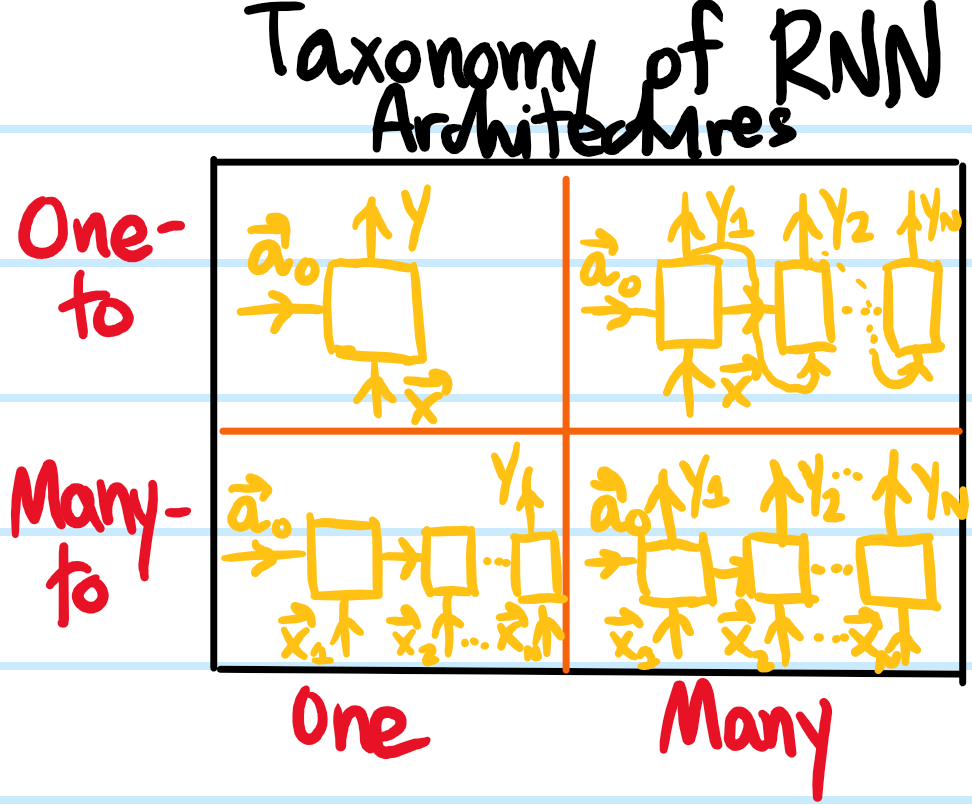
The vanilla RNN architecture described above involving named entity recognition would be classified as a many-to-many RNN architecture.
Problem: Moving on from the example of named entity recognition, consider now a different task of implementing a (word-level) language model using an RNN; how can that be done?
Solution: Using a many-to-many RNN architecture that uses the same hidden state update rule as before:
\[\mathbf a_t=\tanh\left(W_{\mathbf a}\mathbf a_{t-1}+W_{\mathbf x}\mathbf x_t+\mathbf b_{\mathbf a}\right)\]
But instead generates a probability distribution over the vocabulary for the next word will be conditioned on the previous words:
\[\mathbf y_t=\text{softmax}(W_{\mathbf y}\mathbf a_t+\mathbf b_{\mathbf y})\in\mathbf R^{10000}\]
Moreover, one not only initializes \(\mathbf a_{t=1}=\mathbf 0\), but also \(\mathbf x_{t=1}=\mathbf 0\) and for \(t\geq 2\) takes the previous output as the next input \(\mathbf x_t=\mathbf y_{t-1}\). This same architecture can also be used to generate sequences of text, namely by sampling from the softmax probability distribution \(\mathbf y_t\) at each time step \(t=1,2,…,T\).
Problem: Explain why the simple RNN architecture above suffers from both the vanishing gradient and exploding gradient problems.
Solution: This problem is in fact a general curse of deep neural networks (and RNNs tend to be “deep” because each time step \(t=1,2,…,T\) is analogous to \(1\) layer when the RNN architecture is unrolled). Specifically, when computing gradients of loss functions \(\partial L/\partial\boldsymbol{\theta}\), backpropagation (called backpropagation through time (BPTT) in the context of RNNs) requires chaining \(T\) Jacobian matrices together in a neural net \(T\) layers deep, so if these Jacobians have spectral radii which are systematically \(<1\) or \(>1\), then multiplying them together would lead respectively to a vanishing gradient \(\partial L/\partial\boldsymbol{\theta}\to\mathbf 0\) or exploding gradient \(\partial L/\partial\boldsymbol{\theta}\to\mathbf{\infty}\). All this is to say that the simple RNN architecture will tend to have trouble remembering sequence feature vectors \(\mathbf x_{\ll t}\) that happened a long time ago because again for RNNs, time=layers.
Problem: Explain how the gated recurrent unit (GRU) is a more sophisticated RNN architecture that overcomes the above problems.
Solution: At each time step \(t=1,2,…,T\), a GRU is a map \(\mathbf a_t=\text{GRU}(\mathbf a_{t-1},\mathbf x_t)\) that computes the next hidden state via a sequence of \(4\) computations:
1. Reset gate vector \(\mathbf r_t\):
\[\mathbf{r}_t = \sigma(W_{\mathbf r\mathbf a} \mathbf{a}_{t-1}+W_{\mathbf r\mathbf x} \mathbf{x}_t + \mathbf{b}_{\mathbf r})\]
2. Proposal of a candidate hidden state vector \(\tilde{\mathbf a}_t\):
\[\tilde{\mathbf{a}}_t = \tanh(W_{\mathbf a\mathbf a}(\mathbf{r}_t \odot\mathbf{a}_{t-1}) + W_{\mathbf a\mathbf x} \mathbf{x}_t+\mathbf{b}_{\mathbf a})\]
3. Update gate vector \(\mathbf u_t\) (isomorphic to reset gate vector \(\mathbf r\leftrightarrow\mathbf u\)):
\[\mathbf{u}_t = \sigma(W_{\mathbf u\mathbf a} \mathbf{a}_{t-1}+W_{\mathbf u\mathbf x} \mathbf{x}_t + \mathbf{b}_{\mathbf u})\]
4. Final GRU output vector \(\mathbf a_t\) as convex linear combination:
\[\mathbf{a}_t = \mathbf{u}_t \odot \tilde{\mathbf{a}}_t+(\boldsymbol{1} – \mathbf{u}_t) \odot \mathbf{a}_{t-1}\]
In particular, these \(4\) computations of the GRU should be compared with the single computation of a vanilla RNN unit discussed earlier:
\[\mathbf a_t=\tanh\left(W_{\mathbf a}\mathbf a_{t-1}+W_{\mathbf x}\mathbf x_t+\mathbf b_{\mathbf a}\right)\]
By using the reset gate \(\mathbf r_t\) to remember only relevant information, the GRU is able to retain a much longer-term memory of what has already come before it, thereby mitigating the vanishing gradient problem.
Problem: Show that the long short-term memory (LSTM) architecture is another RNN architecture which, like the GRU, also mitigates the vanishing gradient problem.
Solution: Unlike a GRU which has \(4\) computations and only \(2\) gates, an LSTM is a bit more involved in that it uses \(6\) computations with \(3\) gates (historically, GRUs were invented as a simplification of LSTMs).
1. Proposal of candidate cell state:
\[\tilde{\mathbf{c}}_t = \tanh(W_{\mathbf c\mathbf a} \mathbf{a}_{t-1} + W_{\mathbf c\mathbf x} \mathbf{x}_t + \mathbf{b}_{\mathbf c})\]
2. Forget gate:
\[\mathbf{f}_t = \sigma(W_{\mathbf f\mathbf a} \mathbf{a}_{t-1} + W_{\mathbf f\mathbf x} \mathbf{x}_t + \mathbf{b}_{\mathbf f})\]
3. Update gate:
\[\mathbf{u}_t = \sigma(W_{\mathbf u\mathbf a} \mathbf{a}_{t-1} + W_{\mathbf u\mathbf x} \mathbf{x}_t + \mathbf{b}_{\mathbf u})\]
4. Update cell state:
\[\mathbf{c}_t = \mathbf{u}_t \odot \tilde{\mathbf{c}}_t+\mathbf{\mathbf f}_t \odot \mathbf{c}_{t-1}\]
5. Output gate:
\[\mathbf{o}_t = \sigma(W_{\mathbf o\mathbf a} \mathbf{a}_{t-1} + W_{\mathbf o\mathbf x} \mathbf{x}_t + \mathbf{b}_{\mathbf o})\]
6. Update hidden state:
\[\mathbf{a}_t = \mathbf{o}_t \odot \tanh(\mathbf{c}_t)\]
Problem: Whatever happened to the output vector \(\hat{\mathbf y}_t\) in the above discussion of the GRU and LSTM recurrent neural network architectures?
Solution: It’s always there, but the exact formula for it depends on the application of interest in a standard way. Usually, one first computes a linear combination \(W_{\mathbf y\mathbf a}\mathbf a_t+\mathbf b_{\mathbf y}\) of the current hidden state, and then applies some activation function to it that depends in the usual way on the application at hand (e.g. sigmoid for binary classification, softmax for multiclass classification).
Problem: Explain how a bidirectional recurrent neural network (BRNN) is an augmentation to the usual RNN architecture.
Solution: Instead of just doing a forward pass in time \(t=1,2,…,T\) through the sequence of feature vectors \(\mathbf x_1,…,\mathbf x_T\), one can also imagine doing a backward pass in time \(t=T,T-1,…,1\) through the same sequence. That is, a BRNN is just \(2\) independent RNNs with hidden states \(\mathbf a_t\) and \(\mathbf a’_t\) respectively, updating according to some specific architectures but in opposite directions through time \(t\):
\[\mathbf a_t=\text{RNN}(\mathbf a_{t-1},\mathbf x_t)\]
\[\mathbf a’_t=\text{RNN}(\mathbf a’_{t+1},\mathbf x_t)\]
such that the output at each time is given by:
\[\hat{\mathbf y}_t\sim\text{nonlinear}(W_{\mathbf y\mathbf a}\mathbf a_t+W’_{\mathbf y\mathbf a}\mathbf a’_t+b_{\mathbf y})\]
Of course, the catch with using a BRNN is that one must have access to the entire time series \(\mathbf x_1,…,\mathbf x_T\) up to the total duration \(T\) in order to be able to use it.