
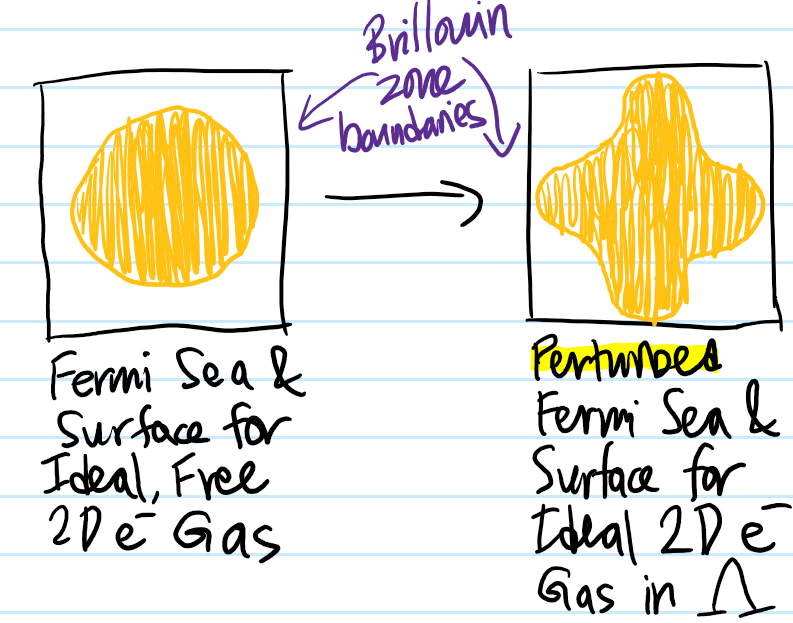
Now suppose that first electron \(e^-\) naturally “burrows” its way down to the ground state \(\textbf n=\textbf k=\textbf 0\) in order to minimize its energy \(E=0\). Now put a second electron \(e^-\) into the box. In reality, the two electrons \(e^-\) would by their mutual Coulomb repulsion run away from each other on a hyperbolic orbit so to speak, raising all energy levels \(E_{\textbf n}\). However, for now we shall ignore all interactions. Then basically we have right now an ideal electron gas of two \(e^-\) that don’t talk to each other. However, actually there is one fundamental quantum mechanical “interaction” so to speak between the two \(e^-\) that cannot be ignored; this is the Pauli exclusion interaction arising from the identical fermionic nature of the spin \(s=1/2\) electrons \(e^-\). Here, as typical, we incorporate spin in an ad hoc manner as just another good quantum number whose associated operators \(\textbf S^2,S_3\) commute with the free space Hamiltonian \(H=T\) of the box. So if the first electron \(e^-\) is in state \(|\textbf n=\textbf 0\rangle\otimes|\uparrow\rangle\), then the second electron \(e^-\), if it also wants to minimize its energy, would have to occupy the state \(|\textbf n=\textbf 0\rangle\otimes|\downarrow\rangle\) (so the total state of the \(2\)-body electron system would be \(|\textbf n=\textbf 0\rangle\otimes|\textbf n=\textbf 0\rangle\otimes\frac{1}{\sqrt 2}(|\uparrow\rangle\otimes|\downarrow\rangle-|\downarrow\rangle\otimes|\uparrow\rangle)\)). The third electron \(e^-\) would then have to live in state \(|\textbf n=(1,0,0)\rangle\otimes|\uparrow\rangle\) for instance and in general we can house \(2\Omega(E_{(1,0,0)})=12\) electrons \(e^-\) in the next energy level, and so forth according to the non-zero values of the scatter plot above. In particular, if one puts in \(N\sim 10^{23}\) electrons for this ideal free electron gas, one would basically fill up a (discrete) ball of electrons in \(\textbf k\)-space (called the Fermi sea) of some radius \(k_F\approx\left(\frac{3N}{8\pi}\right)^{1/3}\), with each lattice point holding two electrons of opposite spin. The spherical boundary \(S^2\) of the Fermi sea of the ideal free electron gas would be called its Fermi surface, whose states thus have momentum \(\hbar k_F\) (called the Fermi momentum) and energy \(E_F=\frac{\hbar^2k_F^2}{2m}\) (called the Fermi energy).
Metals vs. Insulators
In practice, we’re not interested in an empty lattice \(\Lambda=\emptyset\), but rather a non-empty lattice \(\Lambda\neq\emptyset\) such as an atomic lattice in a solid! And what’s more, electrons \(e^-\) don’t just “get added” by some external agent, but rather emerge naturally as the valence electrons \(\partial e^-\) from the atoms located at the lattice sites \(\textbf x\in\Lambda\); thus, working inside a solid kills both birds with one stone.
At a high level, the act of superimposing a Bravais lattice \(\Lambda\) within what used to be an empty cube of sides \(L\) can be treated perturbatively exactly as one does in the nearly free electron model. Specifically, we’re still keeping the ideality/non-interacting assumption between the electrons (with the caveat of the Pauli interaction already mentioned), but now we go from being free\(\rightarrow\)nearly free (used in a technical sense). From that analysis, we know that the presence of the \(\Lambda\)-periodic potential butchers the previous free electron dispersion relation \(E(\textbf k)=\hbar^2|\textbf k|^2/2m\) into an energy band structure \(E_{\text{bands}}(\textbf k)\) where each Brillouin zone \(\Gamma_{\Lambda^*}^{(0)},\Gamma_{\Lambda^*}^{(1)}\), etc. (or bijectively, each energy band \(E_{\text{bands}}(\Gamma_{\Lambda^*}^{(0)}),E_{\text{bands}}(\Gamma_{\Lambda^*}^{(1)})\)) can accommodate precisely \(N\) momentum \(\textbf k\)-states (and thus \(2N\) electrons \(e^-\)) where \(N\) is the number of atoms in the solid. Suppose each atom contributes \(Z\) valence electrons (called its valency). Then the total number of free electrons roaming the solid will be \(ZN\), corresponding to the occupation of \(Z/2\) Brillouin zones or equivalently energy bands. In the ideal free electron case, we saw that the Fermi sea was a ball and its Fermi surface boundary \(\partial=S^2\) a sphere. Now, in the ideal nearly free electron case, we know that the energy is lowered at the boundary \(\partial\Gamma_{\Lambda^*}\) of the Brillouin zones (viewed from “within” otherwise how would the energy band gap form?) so this will distort the Fermi sea (and by extension the Fermi surface \(E_F\)-“equipotential”) of electrons towards it (but conserving in this case the area or in \(3\)D the volume of the Fermi sea since that’s the number of occupied \(\textbf P\)-eigenstates). For \(Z=1\) alkali metal solids or other metals (e.g. \(\text{Li},\text{Cu}\)), the act of “turning” on the perturbation due to the presence of the lattice \(\Lambda\) would look (for a \(2D\) material) something like (because \(Z=1\), the area of the initial Fermi sea/disk must be half the area of the square Brillouin zone):
It is clear in this \(2\)-dimensional case that, if the potential \(V\) induces a sufficiently large energy band gap (as it turns out it does for \(\text{Cu}\)), the Fermi surface can cross the Brillouin zone boundary \(\partial\Gamma_{\Lambda^*}\), though it must do so orthogonally in the reduced scheme to maintain its smoothness by virtue of the toroidal topology \(\Gamma_{\Lambda^*}\cong S^1\times S^1\) of the Brillouin zone.
Now, why do we care about the Fermi surface so much? Short answer: because materials with Fermi surfaces are metals. Qualitatively, the idea is that only the electrons with momentum \(\textbf k\) living on the Fermi surface of the system can actually do anything (having access to a bunch of unoccupied states slightly higher in energy to be able to respond to e.g. an \(\textbf E_{\text{ext}}\) to minimize their energy and form a current \(\textbf J=\sigma\textbf E_{\text{ext}}\)) just as only the valence electrons \(\partial e^-\) could delocalize (except that the former is a “meta-layer” of valency above the latter!). Any electrons \(e^-\) deep in the Fermi sea are pretty much trapped there by the Pauli exclusion principle since there’s no room for them to climb up into nearby energy levels above because they’re already occupied by other electrons (it would take a lot of energy for them to escape)!
For a sense of scale, most metals typically have Fermi temperatures on the order of \(T_F=E_F/k\sim 10^4\text{ K}\) (which is about twice as hot as the surface of the Sun \(\odot\)). This is why Fermi surfaces are also strictly defined at absolute zero \(T=0\), since most real materials in room temperature environments are nowhere near their Fermi temperature \(T_F\).
Another point is that, of course, the number of low-energy excitations available in a metal is proportional to the surface area \(\sim k_F^2\sim E_F\) of its Fermi surface (because each point on the Fermi surface corresponds to an excitable electron \(e^-\)).
Now consider \(Z=2\) atoms (e.g. alkaline earth atoms like \(\text{Be}\)). Now the initial Fermi sea/disk for the ideal free electron system has area equal to the square, but geometrically this implies that it must leak out the boundary of the Brillouin zone a little bit. If one now superimposes the perturbing lattice \(\Lambda\), there are \(2\) possibilities depending on the strength of the periodic lattice potential \(V_{\Lambda}\):
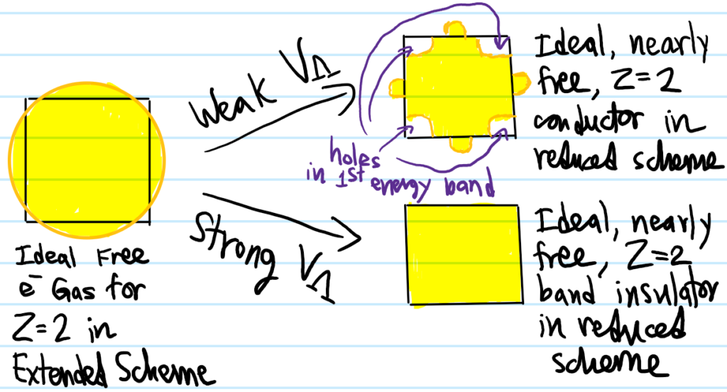
One might think the Fermi surface in the case of band insulators is just the boundary \(\partial\Gamma_{\Lambda^*}\) of the Brillouin zone but that’s not right because it’s not an equipotential with respect to any well-defined Fermi energy \(E_F\).
From here onwards \(Z=3,4,5,…\), the qualitative classification essentially repeats. Metals for instance may have several fully-occupied core bands, a fully-occupied valence band, and then right above that a partially-occupied conduction band. Note though that the Fermi surface need not lie solely in a single Brillouin zone, but can have sections distributed through several Brillouin zones. For example, if we consider the ideal, free electron gas with \(Z=3\) this time (so the area of the circle is three times that of the square \(1\)-st Brillouin zone that it now contains), then:
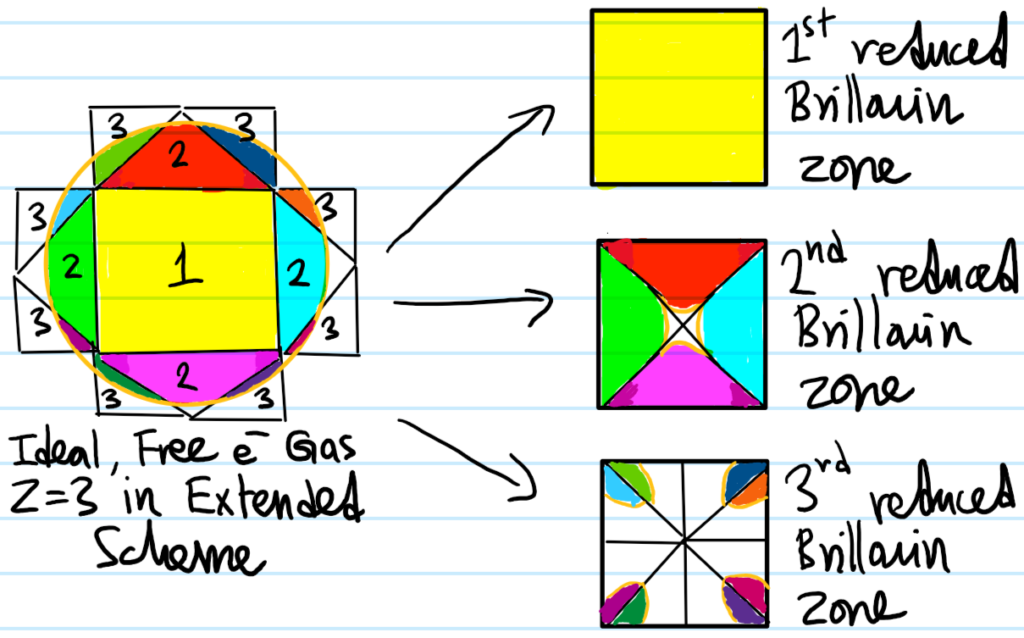
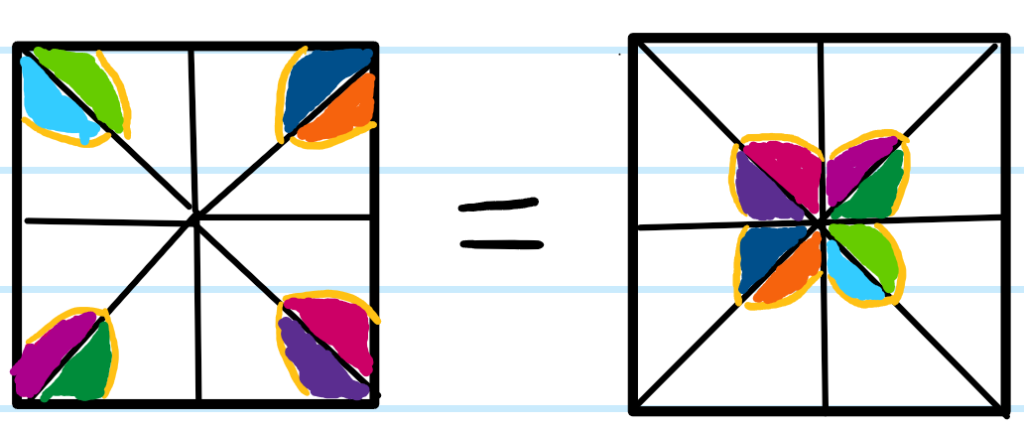
Although the Fermi surface in the \(3\)-rd Brillouin zone square looks disconnected, in fact it is connected (as it was in the extended scheme) because opposite sides of that square in the reduced scheme are topologically glued together (put another way, within the \(3\)-rd Brillouin zone reduced square, if one shifts the “origin” from where it is right now to the top right corner for instance (although all corners are equivalent), then the Fermi surface clearly becomes connected (see this either by tessellating the square or thinking of it as a torus \(S^1\times S^1\) and wrapping the square on itself):
This concludes a qualitative overview of band theory (classification of materials based on whether they are gapped or gapless). While the framework in general is fairly robust, there are some situations where its predictions fail. And as one might suspect, the origin of such deviations are due to one of the assumptions of band theory not being satisfied, notably the assumption of ideality. Examples of these deviations include semiconductors, Mott insulators (cf. band insulators), and topological insulators.
The purpose of this post is to calculate the energy band structure of the famous \(2\)-D material graphene. This of course is a monolayer of carbon \(\text C\) atoms arranged in a hexagonal “honeycomb” lattice. Sheets of graphene stacked on each other are called graphite.

Triangular Lattices, Brillouin Zone, Dirac Points
The first thing to notice is that this hexagonal lattice is non-Bravais because the \(\text C\) atoms are not in identical environments. As usual, this is resolved by viewing it as the convolution of a Bravais triangular lattice \(\Lambda_{\Delta}\) with a motif of \(2\)-carbon atoms dropped at each lattice point of \(\Lambda_{\Delta}\) (strictly speaking, this \(\Lambda_{\Delta}\) that I’m calling “triangular” is also confusingly often called hexagonal in crystallography). Therefore, we use the following primitive lattice vectors \(\textbf x_1,\textbf x_2\) which \(\text{span}_{\textbf Z}(\textbf x_1,\textbf x_2)=\Lambda_{\Delta}\):
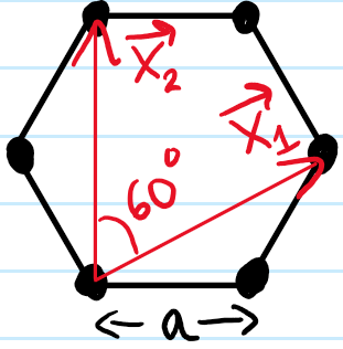
Note that the lengths of the primitive lattice vectors are related to the inter-carbon atom spacing \(a\approx 1.4\) Å by \(|\textbf x_1|=|\textbf x_2|=\sqrt 3a\) and that the area of the spanning parallelogram is \(|\textbf x_1\times\textbf x_2|=\frac{3\sqrt{3}}{2}a^2\). Of course we also have a reciprocal Bravais lattice \(\Lambda^*_{\Delta}\) which is also triangular and spanned by reciprocal lattice vectors \(\textbf k_1,\textbf k_2\in\Lambda^*_{\Delta}\):

where now \(|\textbf k_1|=|\textbf k_2|=\frac{4\pi}{3a}\) and \(|\textbf k_1\times\textbf k_2|=\frac{8\pi^2}{3\sqrt{3}a^2}\) by the defining criterion \(\textbf x_{\mu}\cdot\textbf k_{\nu}=2\pi\delta_{\mu\nu}\). The first Brillouin zone is hexagonal and henceforth we reduce all other Brillouin zones to this:

where the side lengths of the Brillouin zone hexagon are \(\frac{4\pi}{3\sqrt{3}a}\) and thus the area of the Brillouin zone is \(\frac{8\sqrt 3\pi^2}{a^2}\). It turns out for graphene that the corners of the Brillouin zone hexagon are especially interesting points, called the Dirac points \(\textbf k_{\text{Dirac}}^{\pm}\) of graphene. Despite the fact that the Brillouin zone hexagon has \(6\) vertices, there are only really \(2\) physically distinct Dirac points as labelled because the other Dirac points are manifestly connected to them by a reciprocal lattice vector in \(\text{span}_{\textbf Z}(\textbf k_1,\textbf k_2)=\Lambda^*_{\Delta}\) and so are identified modulo the reduced zone scheme.
Physics of Graphene (Tight-Binding)
Each carbon \(\text C\) atom in graphene has valence \(Z=1\) from donating its one \(2p_3\) atomic orbital electron \(e^-\) into a collective \(\pi\) orbital delocalized over the entire graphene sheet. We’ll model these electrons as being tightly bound to carbon \(\text C\) atoms but free to tunnel/hop around the graphene lattice. In general, the tight-binding/hopping Hamiltonian is:
\[H=H(\Lambda_{\Delta},\mathcal M,t_0,t_1,t_2,…)=-\sum_{n=0}^{\infty}t_n\sum_{\textbf x\in\Lambda_{\Delta}}\sum_{\textbf x’\in\Lambda_{\Delta}*\mathcal M:|\textbf x’-\textbf x|_1=n}|\textbf x\rangle\langle\textbf x’|+|\textbf x’\rangle\langle\textbf x|\]
where \(\mathcal M\) is the \(2\)-carbon atom motif at each lattice point in \(\Lambda_{\Delta}\), \(t_n\in\textbf R\) are hopping energy amplitudes for \(n\)-th nearest neighbours, \(|\textbf x’\rangle\langle\textbf x|=(|\textbf x\rangle\langle\textbf x’|)^{\dagger}\) are mutual adjoints which physically permits bidirectional tunneling and mathematically ensures \(H^{\dagger}=H\) is Hermitian, and \(|\textbf x-\textbf x’|_1\) is a taxicab-like metric on the triangular Bravais lattice \(\Lambda_{\Delta}\) which makes it into a metric space, defined as the shortest number of hops between the two points \(\textbf x,\textbf x’\in\Lambda_{\Delta}\) (in graph theoretic terms, this is commonly called the graph geodesic distance between \(\textbf x\) and \(\textbf x’\)). In practice, it is common to restrict to only \(n=0\) (the on-site energy) and \(n=1\) (nearest neighbour) hopping, thereby ignoring all hopping across \(n\geq 2\) atoms. For graphene, the nearest-neighbour hopping energy amplitude turns out to be \(t_1\approx 2.8\text{ eV}\). With this simplification, the tight-binding Hamiltonian becomes (via a resolution of the identity):
\[H\approx -2t_01-t_1\sum_{\textbf x\in\Lambda_{\Delta}}\sum_{\textbf x’\in\Lambda_{\Delta}*\mathcal M:|\textbf x’-\textbf x|_1=1}|\textbf x\rangle\langle\textbf x’|+|\textbf x’\rangle\langle\textbf x|\]
Since the \(n=0\) term \(-2t_01\) is just proportional to the identity \(1\), it doesn’t affect any of the physics so we can ignore it henceforth. For graphene, there are of course \(3\) nearest neighbour carbon atoms \(\textbf x’\in\Lambda_{\Delta}*\mathcal M\) for each carbon atom at position \(\textbf x\in\Lambda_{\Delta}\):
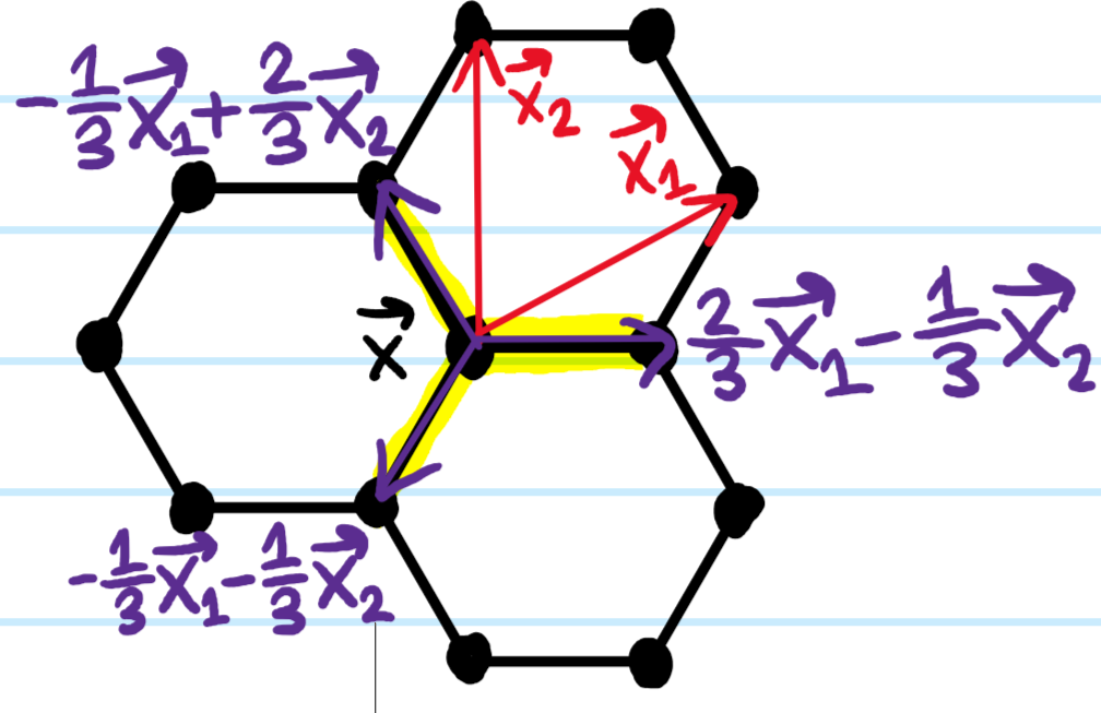
\[H=-t_1\sum_{\textbf x\in\Lambda}|\textbf x\rangle\langle\textbf x+\frac{2}{3}\textbf x_1-\frac{1}{3}\textbf x_2|+|\textbf x\rangle\langle\textbf x-\frac{1}{3}\textbf x_1+\frac{2}{3}\textbf x_2|+|\textbf x\rangle\langle\textbf x-\frac{1}{3}\textbf x_1-\frac{1}{3}\textbf x_2|\]
As usual, we now declare that we wish to solve \(H|E\rangle=E|E\rangle\). For this we’ll simply make a Wannier-type ansatz of the \(H\)-eigenstate \(|E\rangle\) as a sum of plane waves modulated by
\[\]