
Problem #\(1\):
Solution #\(1\):
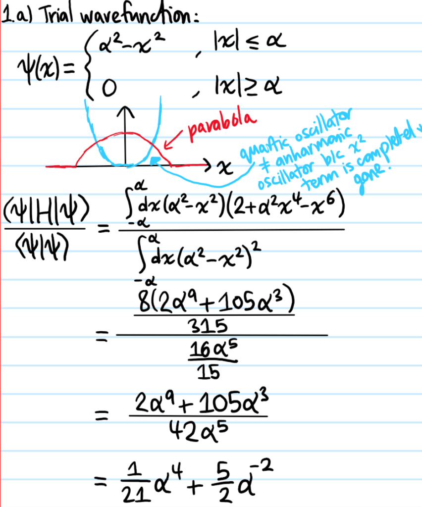
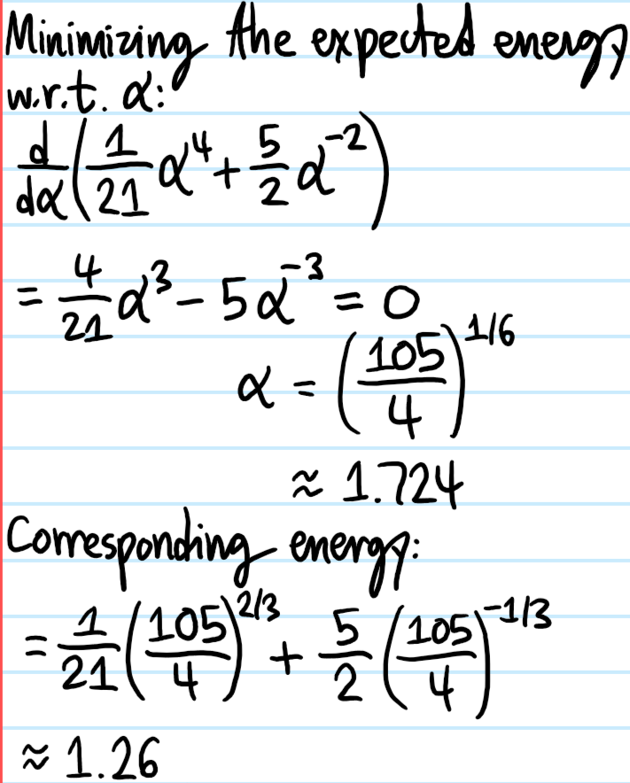
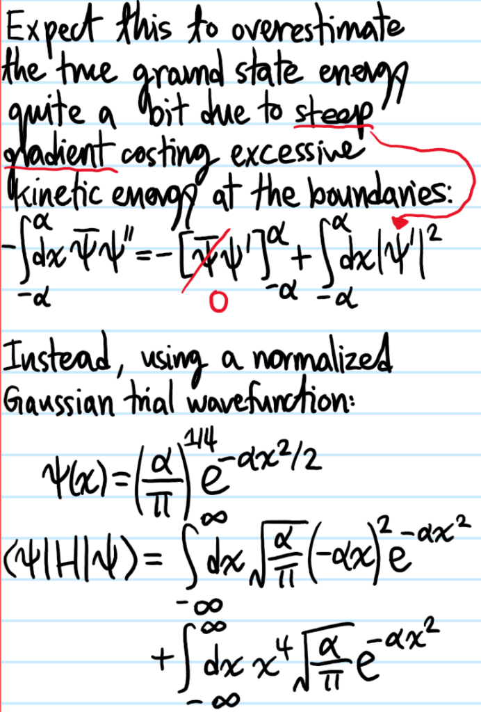
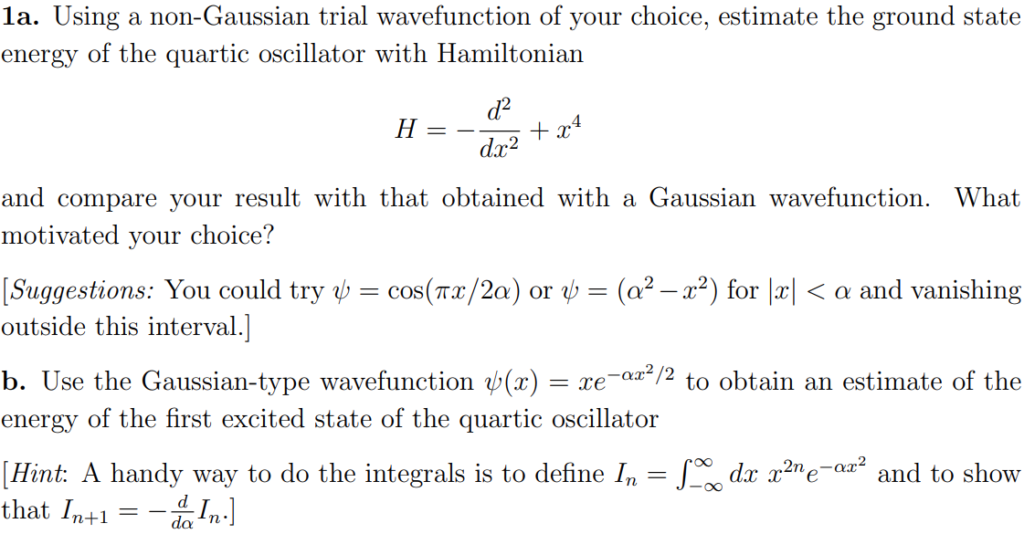
Problem:
Solution:
Problem #\(3\):
Solution #\(3\):
Problem #\(4\):
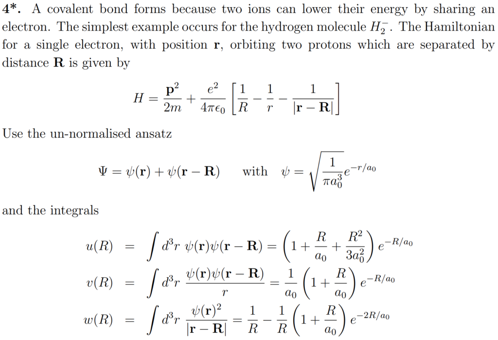
Solution #\(4\):
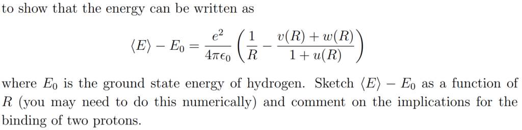
Problem #\(5\):
Solution #\(5\): First, although this tight-binding model looks like a classical model, in fact it arises from the quantum Hamiltonian \(H=E_01-t_1\sum_n(|n+1\rangle\langle n|+|n-1\rangle\langle n|)\) together with the “discrete position representation” \(|\psi\rangle=\sum_n\psi_n|n\rangle\Leftrightarrow\psi_n:=\langle n|\psi\rangle\). The piece \(\psi_{n-1}+\psi_{n+1}\) can be coarse-grained to a kinetic energy:
\[\psi_{n-1}+\psi_{n+1}=\psi_{n-1}+\psi_{n+1}-2\psi_n+2\psi_n\approx\Delta x^2\psi^{\prime\prime}-2\psi\]
to yield the Schrodinger equation for a free particle:
\[-t_1\Delta x^2\psi^{\prime\prime}+(E_0-2t_1)\psi=E\psi\]
with effective mass \(m^*\) defined through \(\frac{\hbar^2}{2m^*}=t_1\Delta x^2\). The eigenstates are the usual scattering plane waves \(\psi(x)\sim e^{\pm ikx}\) where one has the free particle dispersion relation:
\[E=E_0-2t_1+t_1k^2\Delta x^2\]
This motivates how to proceed, namely replace \(x\mapsto n\Delta x\) and make the ansatz \(\psi_n=e^{ikn\Delta x}\). Doing so gives the cosine band dispersion:
\[E=E_0-2t_1\cos k\Delta x\]
so in this tight-binding approximation there is a single band of width \(4t_1\) centered at \(E_0\) (no notion of band gaps in this model because there’s only \(1\) band!). Notice also that Taylor expanding the \(\cos\) reproduces the earlier free particle dispersion near \(k=0\).
For part b), for \(n\leq -1\) or \(n\geq 2\), in both cases one finds:
\[t_1(c+c^{-1})+E-E_0=0\]
Meanwhile for \(n=0,1\), one finds:
\[\begin{pmatrix}s&E-E_0+ct_1\\E-E_0+ct_1&s\end{pmatrix}\begin{pmatrix}\alpha\\\beta\end{pmatrix}=\begin{pmatrix}0\\0\end{pmatrix}\]
this is a \(2\times 2\) circulant matrix so the (unnormalized) eigenvectors \((\alpha,\beta)=(1,\pm 1)\) are very easy to read off and so no determinant computations are even needed; the dispersion relations are \(E-E_0=-ct_1\pm s\). Eliminating \(E-E_0\) in the “bulk” equation immediately yields \(c=\pm t_1/s\) so that \(|c|<1\) which indicates a bound state in which the electron is localized near the origin by the high-energy \(s>t_1\) defect because \(\psi_n\to 0\) as \(n\to\pm\infty\). The energies \(E_{\pm}=E_0\pm\left(\frac{t_1^2}{s}+s\right)\) may be checked to lie outside the original band \(E\in[E_0-2t_1,E_0+2t_1]\).
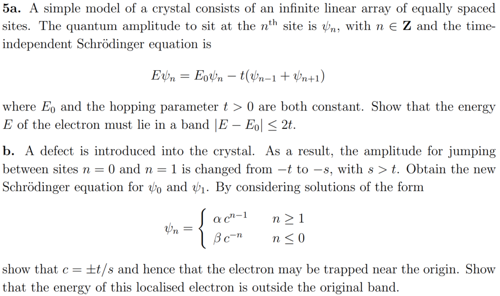
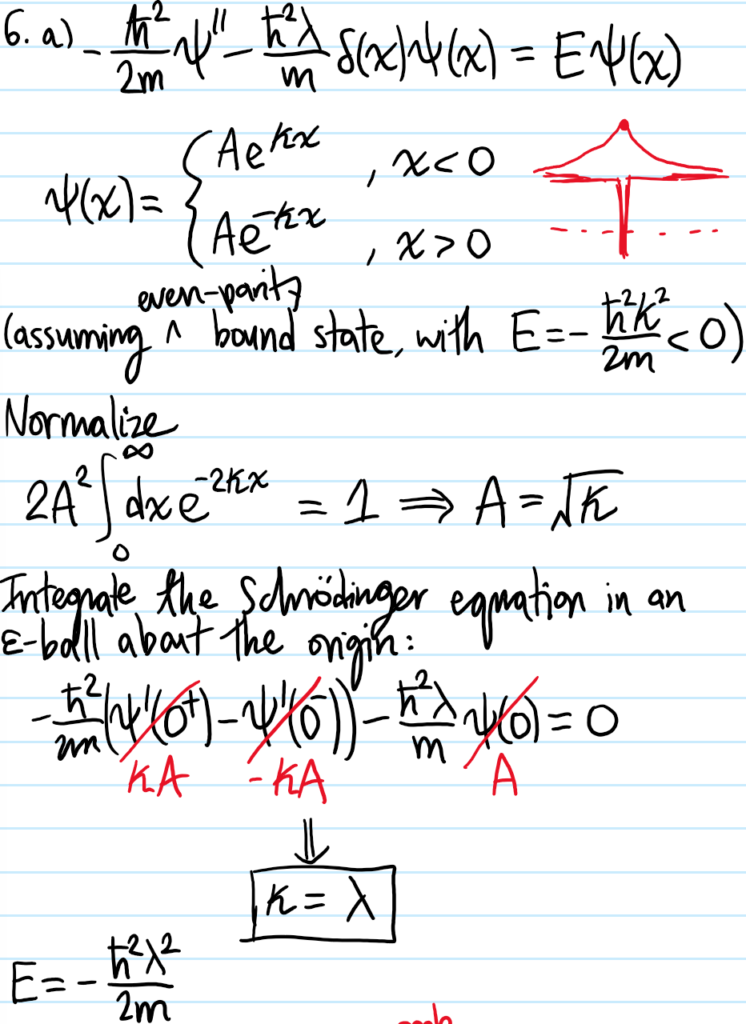
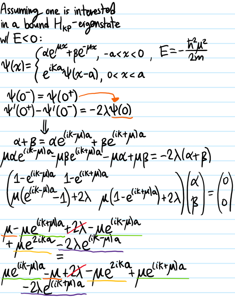
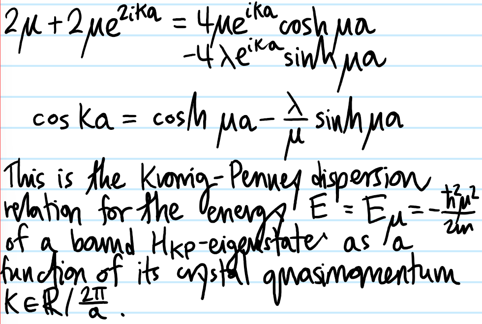
Problem #\(6\):
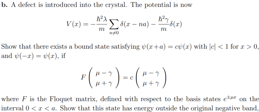
Solution #\(6\):
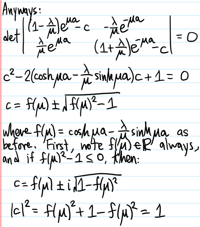
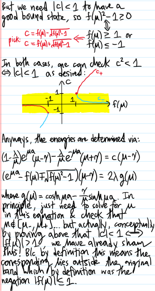
Problem #\(7\):
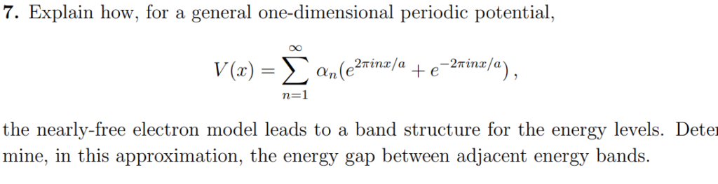
Solution #\(7\):