
Consider an arbitrary worldline \(\{(t,\textbf x)\}\) of a classical system of particles in configuration spacetime. In general, this worldline need not correspond to any physical/on-shell trajectory; it can be as wildly off-shell as one likes, the only caveat being that time travel is forbidden (i.e. it must be possible to parameterize the worldline as \(\textbf x(t)\)).
Now take this worldline \(\{(t,\textbf x)\}\) and gently perturb each point on it \((t_0,\textbf x_0)\mapsto (t_0+\delta t(t_0,\textbf x_0),\textbf x_0+\delta\textbf x(t_0,\textbf x_0))\) by some infinitesimal translation to obtain a slightly shifted worldline. Given any generic off-shell function \(L(t,\textbf x,\dot{\textbf x})\) on configuration spacetime, if the function had value \(L(t_0,\textbf x_0,\dot{\textbf x}_0)\) at some point \((t_0,\textbf x_0)\in\{(t,\textbf x)\}\) on the worldline prior to the perturbation, then after the perturbation the value of the function at the corresponding displaced point \((t_0+\delta t(t_0,\textbf x_0),\textbf x_0+\delta\textbf x(t_0,\textbf x_0))\) on the perturbed worldline would be:
\[L(t_0+\delta t(t_0,\textbf x_0),\textbf x_0+\delta\textbf x(t_0,\textbf x_0),\dot{\textbf x}_0+\delta\dot{\textbf x}(t_0,\textbf x_0))\]
\[\approx L(t_0,\textbf x_0,\dot{\textbf x}_0)+\frac{\partial L}{\partial t}(t_0,\textbf x_0,\dot{\textbf x}_0)\delta t(t_0,\textbf x_0)+\frac{\partial L}{\partial\textbf x}(t_0,\textbf x_0,\dot{\textbf x}_0)\cdot\delta\textbf x(t_0,\textbf x_0)+\frac{\partial L}{\partial\dot{\textbf x}}(t_0,\textbf x_0,\dot{\textbf x}_0)\cdot\delta\dot{\textbf x}(t_0,\textbf x_0)\]
Henceforth dropping the cumbersome arguments (but keeping in mind the equation holds at any arbitrary point \((t_0,\textbf x_0)\in\{(t,\textbf x)\}\) on the unperturbed worldline), one thus has:
\[\delta L=\frac{\partial L}{\partial t}\delta t+\dot{(\textbf p\cdot\delta\textbf x)}+\left(\frac{\partial L}{\partial\textbf x}-\dot{\textbf p}\right)\cdot\delta\textbf x\]
where \(\textbf p:=\frac{\partial L}{\partial\dot{\textbf x}}\). So far this has just been math. At this point, one has to introduce \(2\) key pieces of physics:
- The function \(L(t,\textbf x,\dot{\textbf x})\) is not just some random function, but a special function called the Lagrangian, defined by \(L(t,\textbf x,\dot{\textbf x}):=T(\dot{\textbf x})-V(t,\textbf x)\).
- Among the uncountably infinite ocean of worldlines \(\{(t,\textbf x)\}\) that one could weave through configuration spacetime, the tiny subset of these worldlines that are physical/on-shell are those which satisfy the stationary action principle. This means that for any pair of points \((t_1,\textbf x^*(t_1)),(t_2,\textbf x^*(t_2))\) on such an on-shell worldline \(\textbf x^*(t)\), the action functional
\[S[\textbf x(t)]:=\int_{t_1}^{t_2}dt L(t,\textbf x(t),\dot{\textbf x}(t))\]
is stationary on \(\textbf x^*(t)\) (i.e. \(\delta S[\textbf x^*(t)]=0\)) subject to the constraints that:
- The initial and final times \(t_1,t_2\) are fixed \(\delta t(t_1,\textbf x^*(t_1))=\delta t(t_2,\textbf x^*(t_2))=0\)
- The initial and final configurations \(\textbf x^*(t_1),\textbf x^*(t_2)\) are also fixed \(\delta\textbf x(t_1,\textbf x^*(t_1))=\delta\textbf x(t_2,\textbf x^*(t_2))=\textbf 0\).
This yields the on-shell Euler-Lagrange equations of motion:
\[\dot{\textbf p}=\frac{\partial L}{\partial\textbf x}\]
On the other hand, if one now relaxes the above boundary conditions (which were needed only for formulating the stationary action principle) and instead consider an arbitrary infinitesimal perturbation \((t_0,\textbf x^*(t_0))\mapsto (t_0+\delta t(t_0,\textbf x^*(t_0)),\textbf x^*(t_0)+\delta\textbf x(t_0,\textbf x^*(t_0)))\) of an on-shell trajectory \(\textbf x^*(t)\) (to emphasize again, the boundaries are now free to move!), then the on-shell action \(S^*=S[\textbf x^*(t)]\) changes by the infinitesimal virial:
\[\delta S^*=\int_{t_1}^{t_2}dt\frac{\partial L}{\partial t}\delta t+[\textbf p\cdot\delta\textbf x]^{t_2}_{t_1}\]
Conservation of Momentum for Free Particle
Consider a free particle \(L=\frac{1}{2}m|\dot{\textbf x}|^2\). The Euler-Lagrange equations assert that such a particle moves at constant velocity \(\dot{\textbf x}=\text{const}\). Thus, all straight lines in configuration spacetime are on-shell worldlines because they make the action stationary.
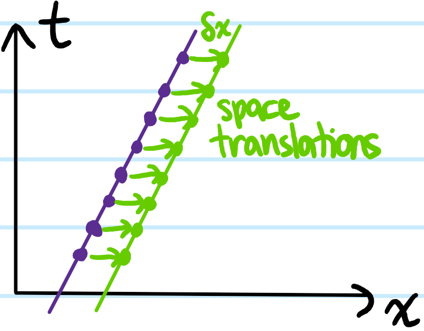
Therefore, if one starts with any such (on-shell) straight worldline \(\textbf x^*(t)\) and performs a simple space translation \(\delta\textbf x\) without any time translation \(\delta t=0\) (purple to green curve), then on the one hand the action is unchanged \(\delta S^*=0\) because the new straight worldline is still on-shell (or mathematically, \(S=\frac{m}{2}\int_{t_1}^{t_2}dt|\dot{\textbf x}(t)|^2\) but the “slope” \(|\dot{\textbf x}|\) didn’t change) but on the other hand general calculus considerations dictate it changes by \(\delta S^*=[\textbf p\cdot\delta\textbf x]^{t_2}_{t_1}\) where \(\textbf p=m\dot{\textbf x}\). One is thus forced to conclude that the quantity \(\textbf p\cdot\delta\textbf x\) (and thus \(\textbf p\) itself because \(\delta\textbf x(t_1,\textbf x(t_1))=\delta\textbf x(t_2,\textbf x(t_2))\) is a uniform space translation) is conserved (since \(t_1\leq t_2\) are arbitrary times). If one likes, this is the integral form of the conservation of momentum. The differential form \(\dot{\textbf p}=\textbf 0\) is just the on-shell Euler-Lagrange equation.
Conservation of Energy for Time-Independent Systems
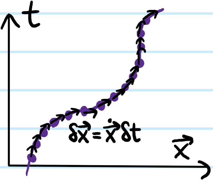
If one perturbs all the points along the curve such that the time and space perturbations are linked by the velocity \(\delta\textbf x=\dot{\textbf x}\delta t\), then this is a symmetry of the system since the on-shell action changes by a boundary term:
\[S^{*’}\approx\int_{t_1+\delta t}^{t_2+\delta t}dt L=\int_{t_1}^{t_2}dt L+\int_{t_2}^{t_2+\delta t}dtL-\int_{t_1}^{t_1+\delta t}dtL\approx S^*+\delta t[L]_{t_1}^{t_2}\]
Making the important assumption that \(\partial L/\partial t=0\), this means that:
\[\delta S^*=\delta t[L]^{t_2}_{t_1}=\delta t[\textbf p\cdot\dot{\textbf x}]_{t_1}^{t_2}\]
from which one obtains the conserved quantity \(H:=\textbf p\cdot\dot{\textbf x}-L\). In differential form, one can check the general on-shell identity \(\dot H=-\frac{\partial L}{\partial t}\) so when \(\frac{\partial L}{\partial t}=0\) one obtains \(H\) as the conserved energy (called the Beltrami identity in the more general setting of the calculus of variations). Strictly speaking \(H\) is not to be confused with the Hamiltonian which is a function of \(\textbf x\) and \(\textbf p\) via a \(\dot{\textbf x}\mapsto\textbf p\) Legendre transform of the Lagrangian \(L\).
Conservation of Angular Momentum
Finally, if the infinitesimal angular translation \(\delta\textbf x:=\delta\boldsymbol{\phi}\times\textbf x\) is a symmetry of the system, then the quantity:
\[\textbf p\cdot(\delta\boldsymbol{\phi}\times\textbf x)=\delta\boldsymbol{\phi}\cdot\textbf L\]
is conserved, where the orbital angular momentum \(\textbf L:=\textbf x\times\textbf p\).
General Remarks on Noether’s Theorem
More generally, anything you can do to some on-shell worldline that keeps it on-shell such that the on-shell action \(\delta S^*\) changes by at most some boundary term (equivalently the Lagrangian \(L\) changes by a total time derivative) is called a symmetry of the system, and this state of affairs can always be rearranged to yield a conservation law. This is Noether’s theorem.
Thus, to recap, Noether’s theorem arises from the fact that the action \(S\) is a time integral \(\int dt\) and that when working on-shell, the variation \(\delta S^*\) in the on-shell action is zero everywhere along the main body of the worldline \(\textbf x^*(t)\) (thanks to the stationary action principle) and so is only sensitive to the “edge effects” associated with changes in the initial and final configurations. But if the perturbation is a symmetry of the system, then one can always reframe this as saying that some quantity is conserved. Implicit in the whole discussion is that these symmetries need to be elements of some continuous Lie group otherwise it wouldn’t be possible to speak of implementing them infinitesimally.
Also, for any kind of purely spatial perturbation \(\delta\textbf x(t)\) so that \(\delta t=0\), it doesn’t even matter if \(\partial L/\partial t\neq 0\)…