
Problem: Explain how to make a Zener diode and the physics underlying its breakdown mechanism.
Solution: A Zener diode is simply made by heavily doping a \(p\)-\(n\) junction, leading to a very thin depletion region. Then, upon applying a suitably strong reverse bias, eventually electrons from the valence band of the \(\text{p}\)-type semiconductor can quantum tunnel into the conduction band of the \(\text n\)-type semiconductor, hence giving rise to Zener breakdown; the Zener voltage at which this occurs is typically \(V_{\text{Zener}}<5\text{ V}\) or so. Beyond this point, a substantial generation current flows across the \(\text p\)-\(\text n\) junction.
Problem: Explain how to make an avalanche diode and the physics underlying its breakdown mechanism.
Solution: The avalanche diode is sometimes also marketed as a Zener diode simply because in practical electronics, both serve the same function, e.g. voltage referencing, protection in flyback Zener diodes, etc.
This time, the idea is to lightly dope instead. One thus gets a large depletion region. Minority mobile charge carriers accelerated across the depletion region then have enough energy to ionize core electrons, leaving behind holes—>3 carriers, each of which is further accelerated by the \(\textbf E\)-field, and can ionize more Si host atoms. This is thus an avalanche effect, leading to avalanche breakdown (e.g. in single-photon avalanche diodes).
Problem: A smartphone tuning app is able to tune the fifth string of a guitar to \(110\text{ Hz}\) with a precision of \(0.07\text{ Hz}\). Estimate the minimum sampling frequency and
sampling time needed for this task.
Solution:
\[f_s\geq 2\times(110+0.07)\text{ Hz}=220.14\text{ Hz}\]
\[T_s\geq\frac{1}{0.07\text{ Hz}}\approx 14\text{ s}\]
Digitization & Signal Processing
In what follows, it is convenient to think of \(f(t)\in\textbf R\) as a real-valued analog \(t\)-domain signal. Then its Fourier transform \(\hat f(\omega):=\frac{1}{\sqrt{2\pi}}\int_{-\infty}^{\infty}f(t)e^{-i\omega t}dt\) (exact convention doesn’t matter) is trivially seen to be conjugate-even in \(\omega\)-space \(\hat f(-\omega)=\hat f^*(\omega)\) and in particular its modulus \(|\hat f(\omega)|\) (which one often plots and speaks of as if it were \(\hat f(\omega)\) itself) is simply an even function in \(\omega\)-space \(|\hat f(-\omega)|=|\hat f(\omega)|\). Thus, as Newton might say, for every positive frequency component \(\omega>0\) in \(\hat f(\omega)\), there is an “equal and opposite” negative frequency component \(-\omega<0\) in \(\hat f(\omega)\). This notion that \(\hat f(\omega)\) will be symmetric around the origin \(\omega=0\) is important to keep in mind in what follows below:
(Weak Nyquist Theorem): Given a \(t\)-domain signal \(f(t)\) whose Fourier transform \(\hat f(\omega)\) is known a priori to be compactly supported (or bandlimited) in \(\omega\)-space on a symmetric interval of the form \([-\omega^*,\omega^*]\), then one can guarantee recovery of \(f(t)\) from the \(t\)-sampled signal \(f(t)Ш_{2\pi/\omega_s}(t)\) at sampling angular frequency \(\omega_s\) (where the Dirac comb is defined by \(Ш_{T}(t):=\sum_{n=-\infty}^{\infty}\delta(t-nT)\)) provided one \(t\)-samples with at least \(\omega_s>2\omega^*\).
Proof: Given the \(t\)-sampled signal \(f(t)Ш_{2\pi/\omega_s}(t)\) at sampling angular frequency \(\omega_s\), the Fourier transform of this product is (by the convolution theorem) the convolution of their Fourier transforms (where the Dirac comb is roughly speaking an eigenfunction of the Fourier transform):
\[f(t)Ш_{2\pi/\omega_s}(t)\mapsto\hat f(\omega)*Ш_{\omega_s}(\omega)\]
which is also equal to \(\hat f(\omega)*Ш_{\omega_s}(\omega)=\sum_{n=0}^{\infty}\hat f(\omega-n\omega_s)\), i.e. placing translated copies of the graph of \(\hat f(\omega)\) at each discrete lattice point \(n\omega_s\) in \(\omega\)-space. No information is lost from sampling if and only if these so-called convolution images \(\hat f(\omega-n\omega_s)\) for \(n\in\textbf Z\) do not overlap with each other in \(\omega\)-space for which it is a sufficient (though not necessary) condition that \(\omega_s> 2\omega^*\) as claimed. More precisely, this claimed losslessness of information is captured by the following explicit algorithm for recovering this information: first, multiplying \(\hat f(\omega)*Ш_{\omega_s}(\omega)\) by the top-hat filter \(\text{rect}(\omega/2\omega^*):=[\omega\in[-\omega^*,\omega^*]]\) in \(\omega\)-space filters out all the duplicate convolution images \(\hat f(\omega-n\omega_s)\) for \(n\neq 0\) arising from the \(t\)-sampling and leaves one with the desired, bandlimited Fourier transform of just the original, unsampled, signal \(f\):
\[\hat f(\omega)=[\hat f(\omega)*Ш_{\omega_s}(\omega)]\text{rect}(\omega/2\omega^*)\]
To recover the original \(t\)-domain signal \(f(t)\), the inverse Fourier transform leads (by the convolution theorem again) to:
\[f(t)=[f(t)Ш_{2\pi/\omega_s}(t)]*2\omega^*\text{sinc}\left(\omega^*t\right)\]
where \(\text{sinc}(x):=\sin(x)/x\) in this context is unnormalized \(\int_{-\infty}^{\infty}\text{sinc}(x)dx=\pi\) (see the Dirichlet integral; one can of course also work with the normalized \(\widehat{\text{sinc}}(x):=\text{sinc}(\pi x)\)) and acts as an interpolating kernel when convolved with the \(t\)-sampled signal \(f(t)Ш_{2\pi/\omega_s}(t)\) (this discussion therefore also proves the Whittaker-Shannon interpolation formula). Hence the information in \(f\) is conserved as promised.
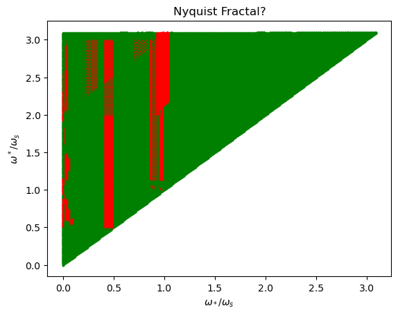
However, given more information about \(f\) (specifically, about \(\hat f\)), one can accordingly do better. That is, suppose \(\hat f(\omega)\) is not merely supported on a symmetric interval in \(\omega\)-space of the form \([-\omega^*,\omega^*]\), but rather on a symmetric union of two intervals of the form \([-\omega^*,-\omega_*]\cup[\omega_*,\omega^*]\) with some lower angular frequency cutoff \(\omega_*<\omega^*\) known a priori in addition to the bandlimiting frequency \(\omega^*\). Then it turns out to be possible to recover \(f(t)\) from a sub-Nyquist \(t\)-sampling frequency \(\omega_s\leq 2\omega^*\) provided one chooses \(\omega_s\) wisely:
(Strong Nyquist Theorem): Given a \(t\)-domain signal \(f(t)\) whose Fourier transform \(\hat f(\omega)\) is known a priori to be bandlimited in \(\omega\)-space on a symmetric union of two intervals of the form \([-\omega^*,-\omega_*]\cup[\omega_*,\omega^*]\), then it may be possible to \(t\)-sample at a sub-Nyquist frequency \(\omega_s>2\Delta\omega\) (where \(\Delta\omega:=\omega^*-\omega_*\) is the bandwidth of the signal \(f\)) while still being able to recover \(f(t)\) from \(f(t)Ш_{2\pi/\omega_s}(t)\).
Proof: Just draw some pictures in \(\omega\)-space. Note the catch to this: such a sampling frequency \(\omega_s\) may not exist if there is not enough room to sneak aliases into the empty region \([-\omega_*,\omega_*]\). The exact nature of when this is possible are complicated:
In practice, for signals \(f(t)\) one encounters in the real world (e.g. temperature \(T(t)\) of a thermistor, air pressure \(p(t)\) of a microphone, displacement \(x(t)\) of a particle, etc. though in practice these are all reduced via modern electronics to voltages \(V(t)\) in a circuit), it is rare to find that \(\hat f(\omega)\) is localized precisely to some interval in \(\omega\)-space like \([-\omega^*,\omega^*]\) or \([-\omega^*,-\omega_*]\cup[\omega_*,\omega^*]\); usually the support \(\hat f^{-1}(\textbf C-\{0\})\) will be unbounded so that in this case the separate convolution images \(\hat f(\omega-n\omega_s)\) separated by the sampling frequency \(\omega_s\) could only be made disjoint from each other in the limit of infinite separation \(\omega_s\to\infty\) in \(\omega\)-space but of course there is no practical \(t\)-sampler with \(\omega_s=\infty\). However all is not lost; in many applications it turns out that one can think of \(\omega_*\) and \(\omega^*\) not as strictly the smallest and largest frequency components present in the signal \(\hat f(\omega)\), but rather as the smallest and largest frequency components in \(\hat f(\omega)\) that one gives a damn about for the application of interest. For instance, human biology limits our ears to being able to detect sound frequencies in between \(\omega_*/2\pi\approx 20\text{ Hz}\) and \(\omega^*/2\pi \approx 20\text{ kHz}\). Mathematically, this means that the signal \(f(t)\) corresponding to \(\hat f(\omega)\) and the signal \(\tilde f(t)\) corresponding to \(\hat f(\omega)\text{rect}_{2\Delta\omega}(\omega)\) sound exactly the same to our ears. The Nyquist theorem therefore asserts that one needs to sample at at least \(\omega_s/2\pi\geq\approx 40\text{ kHz}\) and indeed the standard audio sampling frequency turns out to be \(\omega_s/2\pi=44.1\text{ kHz}\).
Operational Amplifiers
An operational amplifier (op-amp for short) is, as its name suggests, a kind of amplifier. The “operational” part of its name refers to the fact that op-amp circuits can essentially be used to perform various mathematical operations on functions such as addition/subtraction \(\pm\), differentiation \(\frac{d}{dt}\), integration \(\int dt\), etc. The typical schematic of an op-amp is shown below (note there is no widespread convention regarding whether one should draw the non-inverting input \(+\) above or below the inverting input \(-\)):
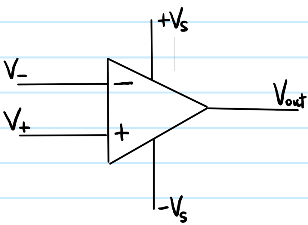
Since op-amps are active components (unlike say resistors, capacitors or inductors which are passive components), they require a bipolar external DC power supply \(\pm V_S\) which is not always annotated on the schematic like it is above, being implicitly understood. Typically, but not always, \(V_S=15\text{ V}\). As far as practical use of op-amps goes, it suffices to treat them as black boxes (in reality lots of transistors, etc.) subject to the following \(3\) rules (strictly true only in the steady state \(t\to\infty\)):
\[V_{\text{out}}\leq V_s\]
\[V_{\text{out}}=A(V_+-V_-)\]
\[I_+=I_-=0\]
where \(A\) is called the op-amp’s open-loop gain because as it stands, the op-amp drawn above is said to be in an open-loop configuration meaning that there’s nothing at all connecting the output \(V_{\text{out}}\) to either of the inputs \(V_{\pm}\) (if there were, then the op-amp would be in a closed-loop configuration). The open-loop gain \(A\) is typically quite large \(A\sim 10^5\), and also not well-controlled during op-amp manufacturing (i.e. there can be a substantially large tolerance \(\Delta A\)). For this reason, despite the fact that the rule \(V_{\text{out}}=A(V_+-V_-)\) clearly suggests an amplification of the differential input voltage \(V_+-V_-\) by the open-loop gain \(A\), actually most of the time (with the exception of certain special op-amp circuits such as comparators), the amplifying ability of the op-amp is not meant to come from its open-loop gain \(A\). Put another way, if one tried to amplify even a mere \(V_+-V_-=0.2\text{ mV}\) using just the raw op-amp in its open-loop configuration, then \(A(V_+-V_-)\sim 20\text{ V}\) would already exceed the typical supply voltage \(V_S=15\text{ V}\), contradicting the first rule and therefore causing the op-amp in this open-loop configuration to simply saturate at \(V_{\text{out}}=V_S=15\text{ V}\).
So as it stands, we have some open-loop op-amp with some large open-loop gain \(A\) plagued by a large uncertainty \(\Delta A\) and only able to amplify the smallest of voltages before saturating. Doesn’t sound too useful! The key insight to addressing all of these problems is, as one may guess, to not be using open-loop op-amps, but rather to use op-amps in a closed-loop configuration. More precisely, there are \(2\) distinct kinds of closed-loop configuration, one generally more useful than the other. If one connects a wire from \(V_{\text{out}}\) to \(V_+\) (resp. \(V_-\)) (possibly with other components like resistors, capacitors, etc. along this wire), then the op-amp is said to be in a positive (resp. negative) feedback configuration. As its name suggests, a positive feedback configuration is self-reinforcing because, suppose initially \(V_+=V_-\) so that \(V_{\text{out}}=0\). Then, if some small perturbation causes a sudden imbalance \(V_+>V_-\), then of course \(V_{\text{out}}=A(V_+-V_-)\) will respond by increasing too. But now comes the positive feedback loop! Since \(V_{\text{out}}\sim V_+\) are correlated together in a positive feedback configuration, as \(V_{\text{out}}\) grows so does \(V_+\) which by \(V_{\text{out}}=A(V_+-V_-)\) causes \(V_{\text{out}}\) to grow even more, and so forth, leading to a runaway instability (in practice the op-amp would quickly rail at \(V_{\text{out}}=V_S\) and square-wave like oscillations of \(\pm V_S\) in \(V_{\text{out}}(t)\) may ensue). This is not very useful unless one is specifically interested in such an oscillator. By far the most useful closed-loop configuration of an op-amp is the negative feedback configuration. Repeating the above arguments shows that this tends to have a stabilizing effect by coaxing \(V_+-V-\to 0\) to a setpoint of \(0\) in a manner not unlike a mass on a spring which attempts to restore the mass’s position \(x\) to the equilibrium position \(x_0\) via \(x-x_0\to 0\). Heuristically:
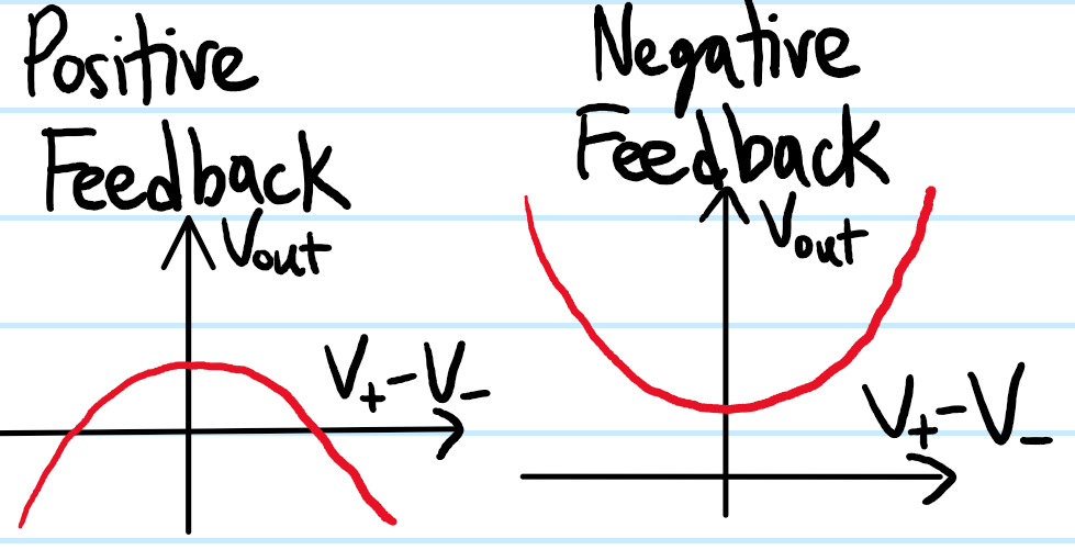
Thus, for op-amps with a closed-loop negative-feedback configuration specifically, one can just assume that \(V_+\approx V_-\) even when \(V_{\text{out}}\neq 0\). This is called the virtual short rule. Together with the two other rules \(V_{\text{out}}\leq V_S\) and \(I_+=I_-=0\), these \(3\) rules taken together are called the golden rules for op-amps (sometimes the rule \(V_{\text{out}}\leq V_S\) is omitted from the golden rules but I think it’s important enough to be included among them). Note that the two golden rules \(V_{\text{out}}\leq V_S\) and \(I_+=I_-=0\) are always true, the former because of just how op-amps work (black box!) and the latter because the input impedance \(Z_+=Z_-=\infty\) is in practice very large, so effectively infinite on both inputs, hence no current is drawn \(I_-=I_+=0\) (this is clearly independent of whether the op-amp happens to be closed-loop or not). But the virtual short golden rule \(V_+=V_-\) only applies to op-amps in closed-loop negative-feedback configurations. This is a very important caveat that one must always remember. In other words, the first thing to always check before analyzing any op-amp circuit is whether or not there is a negative feedback path \(V_{\text{out}}\to V_-\). If so, then one’s life is made easy by the \(3\) golden rules. Otherwise, if the op-amp is in an open-loop or closed-loop but positive-feedback configuration, then one must be more careful and in particular one cannot just blindly apply the golden rule \(V_+=V_-\) anymore.
Perhaps the simplest closed-loop negative-feedback op-amp circuit is that of the voltage follower; one simply starts with an open-loop op-amp and then connects a negative feedback loop \(V_{\text{out}}\to V_-\) with absolutely nothing on it:
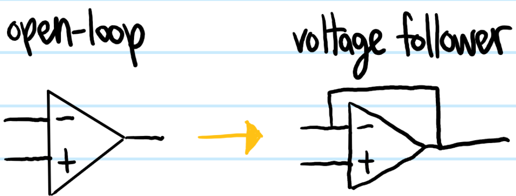
Thanks to the earlier discussion, one can therefore legitimately apply the golden rules here to find that, at equilibrium, \(V_{\text{out}}=V_+=V_-\), hence the name “voltage follower”. It may seem like a voltage follower is a bit of a pointless op-amp circuit because it simply “buffers” the input voltages \(V_+,V_-\) across to the output \(V_{\text{out}}\); after all a wire would do exactly the same thing. The key difference though is that whereas a wire will also draw some non-zero current \(I\neq 0\), a voltage follower, being essentially an op-amp, does not draw any current \(I_+=0\) as one of the op-amp golden rules. In other words, electrons \(e^-\) are allowed to hop between the two stages, so they are effectively isolated from each other and cannot affect each other. This point is best illustrated with the following explicit example in which the first stage is a voltage divider \((R,R)\) (same resistance \(R\) for simplicity) and the second stage is some load resistor \(R\) (again same \(R\) for simplicity). One would like to take the voltage outputted at the center of the voltage divider and apply it across the load resistor \(R\). Naively, applying an input voltage of \(V_{\text{in}}\) across the voltage divider leads to an output voltage \(V_{\text{out}}=V_{\text{in}}/2\). Suppose this is how much voltage we actually would like to apply across the load resistor \(R\). So then we connect the load resistor \(R\) to the voltage divider with a simple, naive wire:
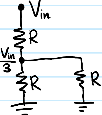
the problem here of course is that the first stage (the voltage divider) is not isolated from the second stage (the load resistor \(R\)) because a current will flow across and into the load resistor \(R\). Because the load resistor \(R\) is in parallel with the bottom resistor \(R\) in the potential divider, one can check this implies that, rather than the voltage divider outputting the voltage \(V_{\text{in}}/2\) we had hoped for, actually it’s been reduced to \(V_{\text{in}}/3\) after we hooked up the load resistor \(R\). Of course in this case it’s not too much hassle to deal with this (just adjust \(V_{\text{in}}\) accordingly), but more generally it can be headache if each additional stage one adds messes with previous stages. Instead of connecting just a bare wire between the two stages, here a voltage follower comes in very handy:
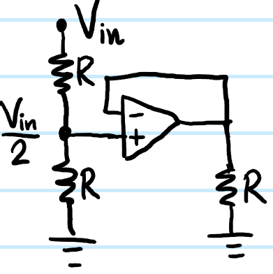
Now, because \(I_+=0\), we recover our expected voltage divider output of \(V_{\text{in}}/2\). Moreover, the voltage follower then simply passes this voltage \(V_{\text{in}}/2\) across the second stage load resistor \(R\) without any fuss, as we desired. Voltage followers therefore provide a simple and effective way to buffer an output voltage from one stage as the input voltage into a second stage, ensuring that any modifications made to the second stage later (e.g. changing the resistance of the load resistor \(R\mapsto R’\neq R\)) do not affect this buffered voltage \(V_{\text{in}}/2\).
Earlier, it was mentioned that op-amps, while possessing amplification powers, are seldom used as open-loop amplifiers with their unstable open-loop gain \(A\). So then how do they amplify voltages? One way is to use an non-inverting amplifier. The idea is to start with the open-loop op-amp, then provide negative feedback through a feedback resistor \(R_F\), followed by completing the voltage divider with a second resistor \(R\) (of course, there are many topologically homeomorphic ways to draw this, in particular drawings that put the non-inverting input \(+\) above the inverting input \(-\)):
The fact that this is a voltage divider for \(V_{\text{out}}\) together with the golden rule (because we’re supplying negative feedback!) immediately yields \(V_{\text{in}}=\frac{R}{R+R_F}V_{\text{out}}\) from which we obtain the equation for a non-inverting amplifier:
\[V_{\text{out}}=\left(1+\frac{R_F}{R}\right)V_{\text{in}}\]
Notice that if one removes the feedback resistor \(R_F=0\), then the non-inverting amplifier reduces to a voltage follower. Notice also that \(1+\frac{R_F}{R}\geq 1\) is always amplifying, never attenuating.
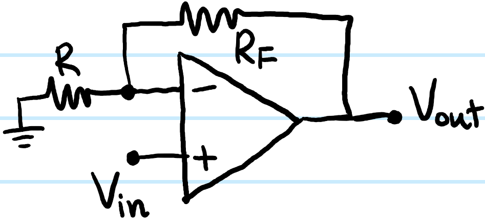
Alternatively, there also exists the inverting amplifier, which derives from the non-inverting amplifier by simply swapping the locations of \(V_{\text{in}}\) and ground \(\text{GND}\):

In this case, equating the currents across the two resistors along the top wire gives the equation for an inverting amplifier:
\[V_{\text{out}}=-\frac{R_F}{R}V_{\text{in}}\]
the fact that \(\text{sgn}(V_{\text{out}})=-\text{sgn}(V_{\text{in}})\) explains why this is called an inverting amplifier (i.e. if \(V_{\text{in}}(t)\) were a time-dependent rather than just DC input voltage, then \(V_{\text{out}}(t)\) would also be time-dependent and \(\pi\) out of phase with \(V_{\text{in}}(t)\)). Actually, the non-inverting and inverting amplifiers together explain why the \(-\) input is called the inverting input in the first place, and likewise why the \(+\) input is called the non-inverting input (see where \(V_{\text{in}}\) is being inputted in the case of each amplifier circuit!). Unlike the non-inverting amplifier, the inverting amplifier can clearly either amplify or attenuate depending on the application. More generally, for any op-amp circuit there will always be some suitable notion of input voltage \(V_{\text{in}}\) along with the usual output voltage \(V_{\text{out}}\) so that for any op-amp circuit one can define its gain \(G:=V_{\text{out}}/V_{\text{in}}\). Thus, a voltage follower has \(G=1\) unit gain, a non-inverting amplifier has gain \(G=1+R_F/R\) while an inverting amplifier has negative gain \(G=-R_F/R\).
In any case, the important point here I want to emphasize again about these amplifier circuits is that, unlike the op-amp’s unstable intrinsic open-loop gain \(A\), these closed-loop gains \(G\) are essentially not functions of \(A\), i.e. \(\partial G/\partial A=0\) precisely because \(A\sim 10^5\) is so large. The point is that \(G\) is a much more controllable gain to work with for amplification purposes than \(A\) because it only depends on the values of external components like resistances \(R_F,R\) which are generally well-known with small tolerances. To hit this point home, consider the following abstraction of the process of negative feedback:
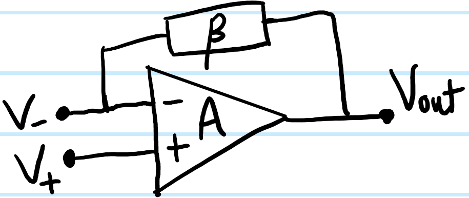
The op-amp is in a closed-loop negative-feedback configuration with a feedback factor \(\beta\in\textbf R\) (implemented through some external components, for instance \(\beta=-R/R_F\) in the inverting amplifier) defined so that it basically does what we intuitively expect negative feedback to do, namely \(V_-\mapsto V_{-}-\beta V_{\text{out}}\). Because \(V_{\text{out}}=G(V_+-(V_{-}-\beta V_{\text{out}}))=A(V_+-V_-)\), it follows that the closed-loop gain \(G\) is related to the open-loop gain \(A\) via:
\[G=\frac{A}{1+\beta A}\]

In particular, because \(A\gg 1\) is large, \(G\approx 1/\beta\) is essentially independent of \(A\)! And even if there’s a large manufacturing uncertainty \(\Delta A\) in the open-loop gain \(A\), the corresponding uncertainty \(\Delta G=\frac{\Delta A}{(1+\beta A)^2}\) in the closed-loop gain \(G\) (assuming \(\Delta\beta\ll\Delta A\) has much less uncertainty which is true) is utterly negligible due to the suppression by a much larger factor of \((1+\beta A)^2\) in the denominator. Intuitively, this is just saying that all the way out at \(A\approx 10^5\), the blue curve is basically flat at \(G\approx 1/\beta\) and so moving around a little bit \(\sim\Delta A\) out so far on such a flat curve won’t really affect the fact that \(G\) is still \(\approx 1/\beta\).
Finally, there is a whole pantheon of clever op-amp circuits that have been devised such as active filters, differentiators, integrators (to make it practical/avoid the DC railing problem, add a shunt resistor in parallel with the capacitor!), summing amplifiers, differential amplifiers, instrumentation amplifiers, comparators, precision rectifiers, \(IV\) converters, Schmitt triggers, etc.
One more point regarding op-amps is that, for AC voltage inputs, their (now complex) open-loop gain \(A=A(\omega)\in\textbf C\) is a function of frequency \(\omega\in\textbf R\), roughly going like \(|A(\omega)|\sim\omega^{-1}\) as \(\omega\to\infty\). On a Bode magnitude plot of \(\log|A(\omega)|\) vs. \(\log\omega\), this behavior shows up as an asymptotic \(\omega\to\infty\) linear behavior with slope \(\frac{d\log|A(\omega)|}{d\log\omega}=-1\). Op-amps are designed with this kind of low-pass open-loop behavior to avoid instabilities at large \(\omega\). In addition to this, one can also add decoupling capacitors \(C_{\text{decoupling}}\) between the external power supply leads \(\pm V_S\) and ground \(\text{GND}\) to short out high-frequency noise that occurs such as when turning on the external DC power supply on (the Heaviside step function \(V_0[t>0]\) has Fourier transform \(V_0\left(\frac{1}{i\omega\sqrt{2\pi}}+\sqrt{\frac{\pi}{2}}\delta(\omega)\right)\)). Finally, one more technicality is that in real life op-amps are also limited by a slew rate \(\dot V_{\text{out}}^*\) such that for all \(t\in\textbf R\), \(|\dot V_{\text{out}}(t)|<\dot V_{\text{out}}^*\) is capped by the op-amp’s slew rate.
Control Systems
A control system may be thought of abstractly as a dynamical system (labelled as just “system” in the block diagrams below) subject to an additional controller input \(\textbf u\) as follows:
\[\dot{\textbf x}=\textbf F(\textbf x,\textbf u)\]
Generalizing the situation for op-amps, there are two kinds of control systems, namely open-loop (also called feedforward) control systems and closed-loop (also called feedback) control systems:
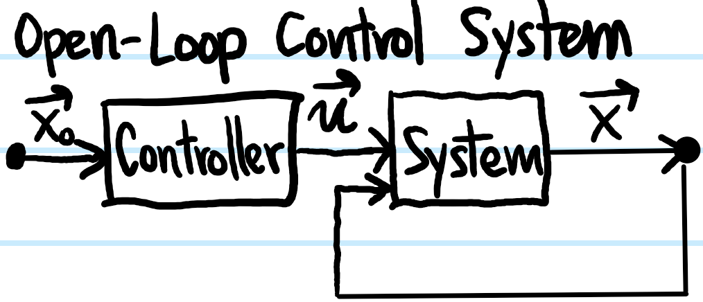
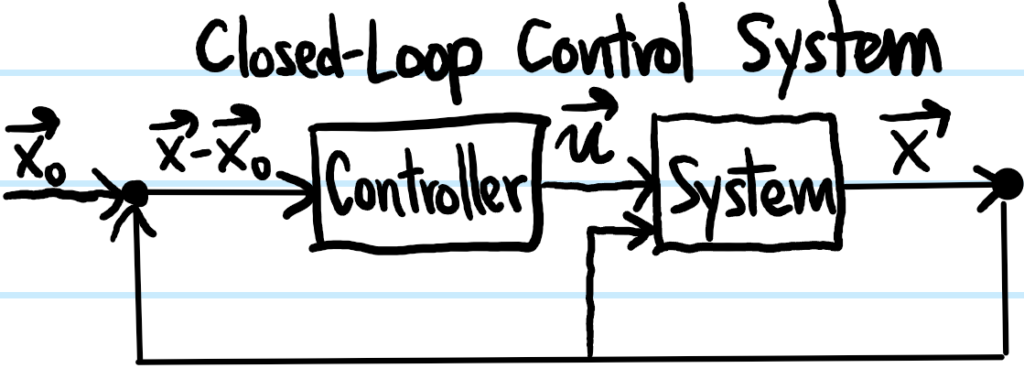
Note that even in the so-called “open-loop control system” there is a closed loop from the output state \(\textbf x\) back into the system. This is just the fact that we’re working with a dynamical system \(\dot{\textbf x}=\textbf F(\textbf x,…)\) where the state at a later time depends on the state at a previous time (we can of course also consider the special case where \(\partial\textbf F/\partial\textbf x=0\) for the system of interest so that there wouldn’t be any such closed loop). This same closed loop also appears in the closed-loop control system, but here the novelty is that there is an additional closed loop (called the control loop!) from the output \(\textbf x\) all the way back into the controller (in the form of the error \(\textbf x-\textbf x_0\) from the desired reference setpoint \(\textbf x_0\)). It is usually this kind of control system possessing a closed control loop in a negative feedback configuration (seeking to minimize \(\textbf x-\textbf x_0\)) that tends to be the most useful. Practically speaking, this is implemented by adding a sensor to continuously the monitor the system’s state \(\textbf x\) and having it feed the measured state \(\textbf x\) back into the controller.
To give an example, one of my pet peeves is traffic lights. Even when there are no cars anywhere in the transverse lane, one must typically still wait out the entire duration of the red light turning green before one can go. In the language introduced above, this is an example of an open-loop control system; the dynamical system consists of the cars approaching this intersection (with state vector \(\textbf x:=(N_1,N_2)\) the number of cars lined up at each intersection) and the controller is the traffic lights. It sucks. To improve this control system, it makes to sense to add a negative feedback control loop (e.g. cameras for counting the number of cars \(N_1,N_2\)). The setpoint state would then be \((N_1,N_2)=(0,0)\).
Focusing on the more interesting case of closed-loop control systems with a negative feedback control loop, one can view the control system in \(\omega\)-space (or engineers also like \(s=i\omega\)-space) rather than the \(t\)-domain. If one assumes that the dynamical system is linear, then one has a block diagram of the form:
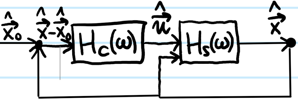
where now \(H_C(\omega)\) is the transfer function of the controller and \(H_S(\omega)\) the transfer function of the dynamical system. Here, because \(\hat{\textbf u}=H_C(\hat{\textbf x}-\hat{\textbf x}_0)\) and \(\hat{\textbf x}=H_S\hat{\textbf u}\), one can eliminate the controller input \(\hat{\textbf u}\) to obtain:
\[\hat{\textbf x}=(H_L-1)^{-1}H_L\hat{\textbf x}_0\]
where \(H_L=H_SH_C\) is the transfer function for the entire control loop.
Whenever \(|H_L|>1\) and \(\text{arg}(H_L)=\pi\), one gets a subcritical Hopf bifurcation (intuitively makes sense but exact details are still muddled). This is like saying that the negative feedback inadvertently becomes positive feedback becomes the application of the negative feedback is \(\pi\)-out of phase with the system’s dynamics, accidentally acting like positive feedback instead. To quantify how far a given (closed-loop, negative-feedback) control system is from this oscillatory instability, one introduces the two complementary notions of the gain margin \(||H_L|-1|_{\arg(H_L)=\pi}\) and phase margin \(|\arg(H_L)-\pi|_{|H_L|=1}\) which are typically straightforward to read off from Bode magnitude and phase plots of the control loop transfer function \(H_L\).
One very popular and effective type of controller is a PID (proportional, integral, derivative) controller which operates on the following formula:
\[\textbf u_{\text{PID}}=K_P\Delta\textbf x+K_I\int_0^t\Delta\textbf x(t’)dt’+K_D\Delta\dot{\textbf x}\]
where \(\Delta\textbf x:=\textbf x-\textbf x_0\) and \(K_P,K_I,K_D\) are constants that typically need to be tuned via trial-and-error.
Noise Filtering
In general, noise \(N(t)\) in the \(t\)-domain may be construed as an uncountable continuum of draws from an uncountable continuum of continuous random variables \(\mathcal N(t)\) that could in principle themselves be \(t\)-dependent (and possibly correlated across different times \(\mathcal N(t)\sim\mathcal N(t’)\)), one draw and one random variable per moment \(t\in\textbf R\) in time (this is often called a stochastic process). Of course, one can also opt to view the noise \(N(t)\mapsto\hat N(\omega)\) in \(\omega\)-space. In this case one often defines \(|\hat N(\omega)|^2\) to be the energy spectral density of the noise \(N\), and because the total energy \(E:=\int_{-\infty}^{\infty}|\hat N(\omega)|^2d\omega=\int_{-\infty}^{\infty}|N(t)|^2dt\) tends to diverge \(E=\infty\) for these kinds of noisy signals \(N\), it is instead more instructive to look at the total power \(P\) of the noise \(N\) instead \(P:=\lim_{\Delta t\to\infty}\frac{1}{\Delta t}\int_{-\Delta t/2}^{\Delta t/2}|N(t)|^2dt=\lim_{\Delta t\to\infty}\frac{1}{\Delta t}\int_{-\infty}^{\infty}|N(t)\text{rect}(t/\Delta t)|^2dt=\lim_{\Delta t\to\infty}\frac{1}{\Delta t}\int_{-\infty}^{\infty}|\hat N(\omega)*\text{sinc}(\omega\Delta t)|^2d\omega\). In particular, the integrand then defines the power spectral density \(\hat P(\omega)=\lim_{\Delta t\to\infty}\frac{1}{\Delta t}|\hat N(\omega)*\text{sinc}(\omega\Delta t)|^2\). Defining the autocorrelation of the noise as \(A(t):=\int_{-\infty}^{\infty}N(t’)N(t’-t)dt’\), a quick calculation via the convolution theorem (assuming a stationary random/Wiener stochastic process which is valid for noise \(N\)) allows one to check that:
\[\hat P(\omega)=\hat A(\omega)\]
The fact that the autocorrelation and the power spectral density are Fourier transform pairs is called the Wiener-Knichin theorem.
There are several different kinds of noise commonly encountered. The simplest is called white noise. This is defined by having a uniform power spectral density \(\hat P_{\text{white}}(\omega)=\text{constant}\). In this case, the Wiener-Knichin theorem asserts that the autocorrelation of white noise is a Dirac delta distribution \(A_{\text{white}}(t)\sim \delta(t)\). This means the only way you get a non-zero correlation is when you put the noise exactly on top of itself; this means that white noise is uncorrelated noise. Examples of white noise include Johnson-Nyquist noise \(\hat P_{\text{JN}}(\omega)\propto T\) in electronics (manage by cooling down electronics) and shot noise in photodiodes.
There is also pink noise which is defined by having a power spectral density which (no pun intended) goes as the power law \(\hat P_{\text{pink}}(\omega)\sim\frac{1}{\omega}\). Roughly speaking, pink noise is universal because it’s associated with self-similarity, similar to a fractal. One simple way to see this self-similarity is that the power allocated to each “octave” (or generalization thereof) is constant for instance:
\[\int_{\omega_1}^{\lambda\omega_1}\hat P_{\text{pink}}(\omega)d\omega=\int_{\omega_2}^{\lambda\omega_2}\hat P_{\text{pink}}(\omega)d\omega\]
for all \(\lambda,\omega_1,\omega_2\in\textbf R\) by virtue of how logarithms work (the autocorrelation for pink noise is also \(A(t)\sim 1/|t|\) if one interprets its power spectral density as \(\hat P_{\text{pink}}(\omega)\sim 1/\omega=1/|\omega|\) symmetrically). Finally, there are also kinds of noise like \(\hat P_{\text{Brownian}}(\omega)\sim 1/\omega^2\).
In practice, it is common to have both white noise and pink noise mixed in with a signal. In the DC limit \(\omega\to 0\), it is clear that pink noise will dominate over white noise \(\hat P_{\text{pink}}(\omega)\gg \hat P_{\text{white}}(\omega)\) but in the high-frequency limit it is white noise that will dominate \(\hat P_{\text{white}}(\omega)\gg \hat P_{\text{pink}}(\omega)\).
Lock-In Detection
A common situation one encounters is that the signal \(f(t)\) one is interested might have some frequency component at some small \(\omega_0\in\textbf R\) so that by the above discussion it will be buried in pink noise. In that case, provided one knows a priori what the frequency \(\omega_0\) of the signal is that one is interested in, then the technique of lock-in detection allows one to lock on to the signal at that frequency \(\omega_0\) notwithstanding even an \(\text{SNR}<1\) (i.e. being buried in the pink noise)! Roughly speaking, lock-in detection just amounts to implementing the Fourier transform \(\hat f(\omega_0)\) evaluated at the frequency \(\omega=\omega_0\) of interest. One starts by having some reference oscillator generate a relatively clean sinusoidal signal \(\sim\cos(\omega_0 t)\) at the frequency \(\omega_0\) of interest. Then, a “mixer” multiplies (or “modulates”) the noisy signal \(f(t)\) by this clean sinusoid (or sometimes a square wave) to obtain \(\sim f(t)\cos(\omega_0 t)\). Finally one needs some kind of low-pass filter to implement an integral-like step \(\sim\int f(t)\cos(\omega_0 t)dt\), which is the usual Fourier transform for \(f\) evaluated at frequency \(\omega_0\) (strictly one has to first also mix in a \(\sim\sin(\omega_0 t)\) reference signal too and repeat everything above). Because the Fourier transform of course not only provides amplitude information \(|\hat f(\omega_0)|\) but also phase information \(\text{arg}\hat f(\omega_0)\), lock-in detection is also sometimes called “phase-sensitive detection”.
Problem: A resistor \(R\) sitting on a table, connected to nothing whatsoever will of course have \(V=0\) across it…or to be more precise, the expected voltage \(\langle V\rangle=0\) will be vanishing, but it turns there will be thermal/equilibrium fluctuations \(\langle V^2\rangle\neq 0\) about \(\langle V\rangle=0\).
Explain heuristically what the origin of such voltage fluctuations \(\langle V^2\rangle\neq 0\) (also called Johnson noise) is and obtain a quantitative estimate of their order of magnitude by equating, in equilibrium, the power dissipated in the resistor with its thermal power from blackbody radiation in the Rayleigh-Jeans limit.
Solution: One has:
\[\frac{\langle V^2\rangle}{(2R)^2}R\sim k_BT\Delta f\]
Hence the RMS voltage is:
\[\sqrt{\langle V^2\rangle}=\sqrt{4Rk_BT\Delta f}\]
where the factor of \(4\) comes from a more detailed analysis (e.g. see Nyquist’s \(1928\) paper about this). In fact, Johnson noise is just a corollary of the fluctuation-dissipation theorem.