Problem: Explain what is meant by a classical field.
Solution: A classical field is any function \(\phi(x)\) (denoted as \(\phi\) because “phi” sounds like “field”) on spacetime \(x:=(ct,\mathbf x)\in\mathbf R^{1,3}\) which is a \(c\)-number, that is to say \(\phi(x)\in\mathbf R\) or \(\phi(x)\in\mathbf C\) or \(\phi(x)\in\mathbf R^4\) or \(\mathbf C^4\) or something like that. Classical fields stand in sharp contrast to quantum fields which are no longer (necessarily) \(c\)-numbers but in general \(q\)-numbers (operator-valued).
Problem: Explain why the words “theory” and “action” are interchangeable, so e.g. if someone says “Klein-Gordan field theory is Lorentz invariant” or “Maxwell’s field theory of classical electromagnetism is both Lorentz invariant and gauge invariant”, it is respectively synonymous with “the Klein-Gordan action is Lorentz invariant” or “the Maxwell action is both Lorentz invariant and gauge invariant”.
Solution: Because once an action \(S\) is written down for a classical field theory, it defines what classical fields are involved in the theory, their dynamics, etc. in other words, a complete specification of all the relevant information.
Problem: Write down the action \(S\) of a classical field theory in terms of its Lagrangian density \(\mathcal L\). State the Lagrangian density \(\mathcal L_{\text{KG}}\) of Klein-Gordan field theory and the Lagrangian density \(\mathcal L_{\text{EM}}\) of Maxwell field theory.
Solution: From classical particle mechanics, \(S=\int dt L\) where \(L=\int d^3\mathbf x\mathcal L\) is the classical Lagrangian. Thus, overall \(S=c^{-1}\int d^{1+3}x\mathcal L\) where the extra factor of \(c\) is to remove the factor of \(c\) in the spacetime measure \(d^{1+3}x=cdtd^3\mathbf x\). Klein-Gordon field theory governs the dynamics of a single real scalar field \(\phi(x)\):
\[\mathcal L_{\text{KG}}(\phi,\partial_0\phi,\partial_1\phi,\partial_2\phi,\partial_3\phi)=\frac{1}{2}\partial^{\mu}\phi\partial_{\mu}\phi-\frac{1}{2}k^2_c\phi^2=\frac{1}{2c^2}\left(\frac{\partial\phi}{\partial t}\right)^2-\left(\frac{1}{2}\left|\frac{\partial\phi}{\partial\mathbf x}\right|^2+\frac{1}{2}k_c^2\phi^2\right)\]
where \(k_c=2\pi/\lambda_c\) is the Compton wavenumber associated to the Compton wavelength \(\lambda_c=h/mc\). The important point is that \(k_c\propto m\). By contrast, Maxwell field theory governs the dynamics of a \(4\)-vector field \(A^{\mu}(x)\):
\[\mathcal L_{\text{EM}}(A^0,A^1,A^2,A^3,\partial…)=-\frac{1}{4\mu_0}F_{\mu\nu}F^{\mu\nu}-J^{\mu}A_{\mu}=\frac{\varepsilon_0}{2}|\mathbf E|^2-\left(\frac{|\mathbf B|^2}{2\mu_0}+\rho\phi-\mathbf J\cdot\mathbf A\right)\]
where the electromagnetic field tensor \(F_{\mu\nu}=\partial_{\mu}A_{\nu}-\partial_{\nu}A_{\mu}\).
Problem: What does it mean for a classical field theory to be Lorentz invariant (aka relativistic)? How can one often instantly tell if a classical field theory is compatible with special relativity or not?
Solution: Loosely speaking, a classical field theory is Lorentz invariant iff its action \(S\) is a Lorentz scalar:
\[\frac{\delta S}{\delta SO^+(1,3)}=0\]
Both Klein-Gordan and Maxwell are relativistic field theories. The giveaway is the presence of Greek spacetime indices like \(\mu,\nu=0,1,2,3\), etc. in their Lagrangian densities \(\mathcal L_{\text{KG}},\mathcal L_{\text{EM}}\) (one calls this phenomenon manifest Lorentz invariance). More precisely, such spacetime indices must be contracted appropriately, thus putting space and time on equal footing.
Problem: More generally, any transformation \((x,\phi_i)\mapsto (x’,\phi’_i)=(x+\delta x,\phi_i+\delta\phi_i)\) of the spacetime coordinates and fields that leaves the action \(S\) invariant is called a symmetry of the classical field theory (perhaps that’s why the action is denoted by the letter \(S\) because it’s screaming “\(S\)ymmetry!”). Explain why finding symmetries is useful.
Solution: If the symmetry is continuous, then Noether’s theorem asserts existence of a conserved \(4\)-current. Moreover, the proof is constructive:
\[\delta S=\frac{1}{c}\int\left(\delta(d^{1+3}x)\mathcal L+d^{1+3}x\delta\mathcal L\right)\]
where the Jacobian determinant is \(\det\left(\frac{\partial x’}{\partial x}\right)\approx 1+\partial_{\mu}\delta x^{\mu}\) and \(\delta\mathcal L=\frac{\partial\mathcal L}{\partial\phi_i}\delta\phi_i+\frac{\partial\mathcal L}{\partial(\partial_{\mu}\phi_i)}\partial_{\mu}\phi_i+\frac{\partial \mathcal L}{\partial x^{\mu}}\delta x^{\mu}=\partial_{\mu}(\pi^{\mu}_i\delta\phi_i)+(\partial_{\mu}\mathcal L)\delta x^{\mu}\) (where \(\pi^{\mu}_i:=\frac{\partial\mathcal L}{\partial (\partial_{\mu}\phi_i)}\)). Hence, the action variation is the spacetime integral of a spacetime divergence:
\[\delta S=\frac{1}{c}\int d^{1+3}x\partial_{\mu}(\pi^{\mu}_i\delta\phi_i+\mathcal L\delta x^{\mu})=0\]
yielding the conserved Noether current:
\[j^{\mu}=\pi^{\mu}_i\delta\phi_i+\mathcal L\delta x^{\mu}\]
Here, \(\delta\phi_i:=\phi’_i(x)-\phi_i(x)\) is the local variation of \(\phi_i\) at a fixed event \(x\in\mathbf R^{1,3}\). It can be related to the net variation \(\Delta\phi_i:=\phi’_i(x’)-\phi_i(x)\) due to both internal transformations and induced variation arising from the coordinate transformation \(\delta x\) using \(\delta\phi_i=\Delta\phi_i-\delta x^{\mu}\partial_{\mu}\phi_i\). This allows the Noether current to be rewritten:
\[j^{\mu}=\pi^{\mu}_i\Delta\phi_i-T^{\mu}_{\nu}\delta x^{\nu}\]
with canonical stress-energy tensor field \(T^{\mu}_{\nu}=\pi^{\mu}_i\partial_{\nu}\phi_i-\delta^{\mu}_{\nu}\mathcal L\) or equivalently \(T^{\mu\nu}=\pi^{\mu}_i\partial^{\nu}\phi_i-g^{\mu}_{\nu}\mathcal L\)
(in particular, notice that \(\delta\mapsto g\)).
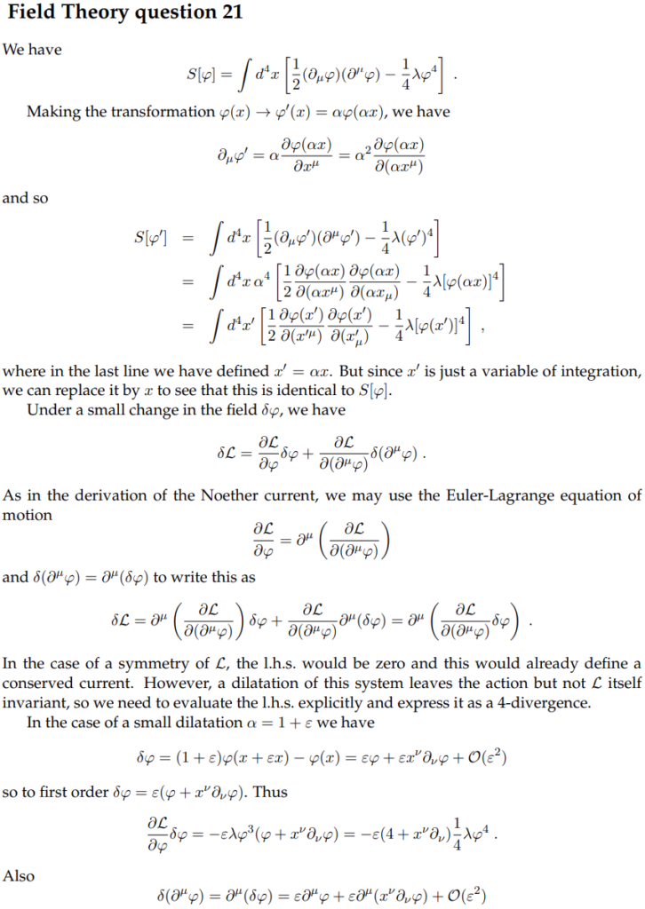
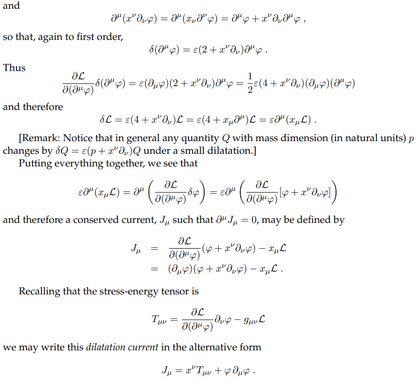
Problem: Consider a classical field theory (massless \(\phi^4\)) involving a single real scalar field \(\phi(x)\) with action:
\[S=\frac{1}{c}\int d^{1+3}x\left(\frac{1}{2}\partial^{\mu}\phi\partial_{\mu}\phi-\frac{\lambda}{4}\phi^4\right)\]
Show that the conformal dilatation transformation \(\phi(x)\mapsto\alpha\phi(\alpha x)\) for \(\alpha\in\mathbf R\) is a continuous symmetry of this classical field theory, and hence compute the associated Noether current.
Solution: The hardest part of this problem is to understand precisely what the notation \(\phi(x)\mapsto\alpha\phi(\alpha x)\) means. The answer is that it simultaneously defines a spacetime transformation \(x\mapsto x’=x/\alpha\) and a corresponding active field transformation \(\phi(x)\mapsto \phi'(x)=\alpha\phi(\alpha x)\), so in particular \(\phi'(x’)=\alpha\phi(x)\). To check invariance of the action \(S\):
\[S’=\frac{1}{c}\int d^{1+3}x’\left(\frac{1}{2}\partial’^{\mu}\phi'(x’)\partial’_{\mu}\phi'(x’)-\frac{\lambda}{4}\phi’^4(x’)\right)\]
\[=\frac{1}{c}\int\frac{d^{1+3} x}{\alpha^4}\left(\frac{1}{2}\alpha\partial^{\mu}(\alpha\phi(x))\alpha\partial_{\mu}(\alpha\phi(x))-\frac{\lambda}{4}\alpha^4\phi^4(x)\right)\]
\[=S\]
One can then linearize about \(\alpha=1\):
\[x’\approx x+(\alpha-1)\left(-\frac{x}{\alpha^2}\right)_{\alpha=1}=2x-\alpha x\]
\[\phi'(x)\approx\phi(x)+(\alpha-1)(\phi(\alpha x)+\alpha x^{\nu}\partial_{\nu}\phi(\alpha x))_{\alpha=1}=\phi(x)+(\alpha-1)(\phi+x^{\nu}\partial_{\nu}\phi)\]
\[\phi'(x’)=\phi(x)+(\alpha-1)\phi(x)=\alpha\phi\]
Thus:
\[\delta x=(1-\alpha)x\]
\[\delta\phi=(\alpha-1)(\phi+x^{\nu}\partial_{\nu}\phi)\]
\[\Delta\phi=(\alpha-1)\phi\]
which is consistent with \(\Delta\phi=\delta\phi+\delta x^{\nu}\partial_{\nu}\phi\). The conserved Noether current is thus (using the form with the stress-energy tensor):
\[j^{\mu}=\partial^{\mu}\phi(\alpha-1)\phi-T^{\mu}_{\nu}(1-\alpha)x^{\nu}\]
Dividing out the infinitesimal \(\alpha-1\):
\[j^{\mu}=\phi\partial^{\mu}\phi+T^{\mu}_{\nu}x^{\nu}\]
(aside: it is instructive to explicitly check \(\partial_{\mu}j^{\mu}=0\) by working on-shell \(\partial^{\mu}\partial_{\mu}\phi=-\lambda\phi^3\) and also invoking spacetime translational symmetry \(\partial_{\mu}T^{\mu}_{\nu}=0\)).
Problem: Continuing with the classical massless \(\phi^4\) field theory:
\[S=\frac{1}{c}\int d^{1+3}x\left(\frac{1}{2}\partial^{\mu}\phi\partial_{\mu}\phi-\frac{\lambda}{4}\phi^4\right)\]
Show that the alternative transformations:
- \(x’=x\), \(\phi'(x’)=\alpha\phi(\alpha x)\)
- \(x’=\cos(\alpha x\), \(\phi'(x’)=\phi(\alpha x)\)
also preserve the action \(S\), hence are symmetries of the theory. Compute their associated Noether currents.
Solution:
- This perspective is implicitly adopted in the Cambridge Theoretical Physics course official solution for this problem:
However, since \(\delta x=0\), this approach suggests an incorrect Noether current \(j^{\mu}=\pi^{\mu}\delta\phi=\phi\partial^{\mu}\phi+x^{\nu}\partial_{\nu}\phi\partial^{\mu}\phi\). Rather, as the solution above suggests, one has to compute the corresponding change in the infinitesimal action \(d^{1+3}x’\mathcal L’-d^{1+3}x\mathcal L=d^{1+3}x(\alpha-1)\partial_{\mu}(x^{\mu}\mathcal L)\), hence giving the required subtractive correction.
2. This transformation is just a trivial renaming of the integration dummy variable from \(x\) to \(x’=\alpha x\) (indeed, it could be renamed to any reasonable \(x’=f_{\alpha}(x)\) with corresponding \(\phi'(x’)=\phi(f_{\alpha}(x))\)):
\[\frac{1}{c}\int d^4x’\mathcal L(\phi(x’),\partial’\phi(x’))=\frac{1}{c}\int d^4x\mathcal L(\phi(x),\partial\phi(x))\]
In particular, \(\phi'(x)=\phi(x)\) and thus \(\delta\phi=0\). The transformation of course has nothing to do with the conformal dilatation of the massless \(\phi^4\) field. Contrary to the previous situation, the formula now predicts an incorrect Noether current \(j^{\mu}=x^{\mu}\mathcal L\). Applying the same correction as above yields the trivial Noether current \(0\).
The lesson here is that one should always write the transformed field \(\phi'(x’)\) in terms of \(\phi(x)\), and in particular not \(\phi(\alpha x)\) or any other \(\phi(f(x))\). Then the earlier Noether current result applies.
Problem: Explain how to calculate the orbital angular momentum pseudovector \(\mathbf L\) of a classical field.
Solution: Recall that spatial rotations \(SO(3)\) form a subgroup of the Lorentz group \(SO^+(1,3)\). Thus, when traditionally working with an infinitesimal Lorentz transformation \(\Lambda^{\mu}_{\nu}=\delta^{\mu}_{\nu}+\omega^{\mu}_{\nu}\), this procedure simultaneously yields conservation laws for both spatial rotations and Lorentz boosts. One has \(\Lambda\in SO^+(1,3)\) iff the generator \(\omega_{\mu\nu}=-\omega_{\nu\mu}\) is antisymmetric (hence denoted by the symbol “\(\omega\)”). Thus, \(x’^{\mu}=\Lambda^{\mu}_{\nu}x^{\nu}\approx x^{\mu}+\omega^{\mu}_{\nu}x^{\nu}\) and \(\Delta\phi=0\) because \(\phi'(x’)=\phi(x)\) is a scalar field. One has:
\[j^{\mu}=-T^{\mu}_{\nu}\omega^{\nu}_{\rho}x^{\rho}=-\omega_{\nu\rho}x^{\rho}T^{\mu\nu}:=\frac{\omega_{\nu\rho}cL^{\mu\nu\rho}}{2}\]
where the orbital angular momentum density tensor field is \(L^{\mu\nu\rho}:=c^{-1}(x^{\nu}T^{\mu\rho}-x^{\rho}T^{\mu\nu})\). There are \(6\) combinations of \(\nu,\rho\in\{0,1,2,3\}\) for which \(\omega_{\nu\rho}\neq 0\), giving \(6\) conserved currents \(\partial_{\mu}L^{\mu\nu\rho}=0\), with the conserved charge \(L^{\mu\nu}=\int d^3\mathbf x L^{0\mu\nu}(x)\). By antisymmetry \(L^{\nu\mu}=-L^{\mu\nu}\), the spatial parts can be identified with a \(3\)-vector in the usual way \(L^i:=\frac{\varepsilon_{ijk}}{2}L^{jk}\); this is the orbital angular momentum pseudovector \(\mathbf L\) of the field.
Problem: Consider a classical field theory involving a complex scalar field \(\psi(x)\). Write down the Lagrangian density \(\mathcal L(\psi)\) for \(\psi\) such that:
\[\mathcal L(\psi)=\mathcal L_{\text{KG}}(\sqrt{2}\text{Re}\psi)+\mathcal L_{\text{KG}}(\sqrt{2}\text{Im}\psi)\]
where the Klein-Gordon Lagrangian density for a real scalar field \(\phi(x)\) is \(\mathcal L_{\text{KG}}(\phi):=\frac{1}{2}\partial^{\mu}\phi\partial_{\mu}\phi-\frac{1}{2}k_c^2\phi^2\). Suppose \(\psi\) is coupled to an electromagnetic field \(A^{\mu}\); describe how \(\mathcal L(\psi)\) needs to be modified to account for this.
Solution: It’s just a “Hermitian” version of Klein-Gordon, without the factors of \(1/2\):
\[\mathcal L(\psi)=(\partial^{\mu}\psi)^{\dagger}\partial_{\mu}\psi-k_c^2|\psi|^2\]
Typically one just writes \((\partial^{\mu}\psi)^{\dagger}=\partial^{\mu}\psi^{\dagger}\) because \((\partial^{\mu})^{\dagger}=\) is Hermitian, but it will soon be important to remember that the dagger \(\dagger\) is meant to act on the entire object.
When \(\psi\) is coupled to an electromagnetic \(4\)-potential \(A^{\mu}\), there are \(2\) changes one must make to \(\mathcal L(\psi)\); the obvious one is to also tack on \(\mathcal L_{\text{EM}}=-F^{\mu\nu}F_{\mu\nu}/4\mu_0\). The more subtle one is the minimal coupling substitution in the kinetic term \(\partial\mapsto\mathcal D:=\partial-iqA/\hbar\) with \(\mathcal D\) the gauge covariant derivative.
Although inspired by the classical minimal coupling \(\mathbf p\mapsto\mathbf p-q\mathbf A\), the reason for this has to do with desiring \(\mathcal L\) to be invariant under a simultaneous local \(U(1)\) phase transformation of the complex scalar field \(\psi(x)\mapsto\psi'(x’)=e^{i\theta(x)}\psi(x)\) in conjunction with a gauge transformation of \(A(x)\mapsto A'(x’)=A(x)+\frac{\hbar}{q}\partial\theta(x)\) (in both cases, \(x’=x\)), then:
\[\mathcal D’\psi’=e^{i\theta}\mathcal D\psi\]
Thus, the kinetic term is invariant \((\mathcal D’\psi’)^{\dagger}\mathcal D’\psi’=e^{-i\theta}e^{i\theta}(\mathcal D\psi)^{\dagger}\mathcal D\psi=(\mathcal D\psi)^{\dagger}\mathcal D\psi\). Equivalently, one can say that if the gauge field is transformed as \(A\mapsto A+\partial\Gamma\), then the scalar field must transform with a local phase \(\psi\mapsto e^{iq\Gamma/\hbar}\psi\).
Problem: Consider the ungauged Lagrangian density:
\[\mathcal L=(\partial^{\mu}\psi)^{\dagger}\partial D_{\mu}\psi-V(\psi)\]
Consider using the Mexican hat potential \(V(\psi)=-k_c^2|\psi|^2+\frac{\lambda}{2}|\psi|^4\) with \(k_c^2,\lambda>0\). Explain both of these inequalities.
Write down the general ground state \(\psi_0\), and “quadraticize” (cf. “linearize”) \(\mathcal L\) about \(\psi_0\). Identify the massless Goldstone field. By promoting global to local \(U(1)\) phase symmetry to hold for the theory, the idea of coupling to a gauge field \(A(x)\) emerges naturally (scalar electrodynamics):
\[\mathcal L=(\mathcal D^{\mu}\psi)^{\dagger}\mathcal D_{\mu}\psi-V(\psi)+\frac{1}{4\mu_0}F^{\mu\nu}F_{\mu\nu}\]
Show that the gauge field \(A(x)\) acquires a mass by eating the Goldstone field via the abelian Higgs mechanism.
Solution: The need to make \(\lambda>0\) arises from insisting that \(V(\psi)\in\mathbf R\) is bounded from below (otherwise \(|\psi|\to\infty\) would be unphysical), so in particular at least \(1\) global minimum exists (called a ground field/”state”). In addition, the negative coefficient \(-k_c^2\) on the quadratic term is the opposite of the positive coefficient \(k_c^2\) that normally appears in Klein-Gordan type Lagrangian densities; this is to mimic ordering behavior in contexts like continuous phase transitions where \(T<T_c\)).
By insisting \(\partial V/\partial |\psi|^2=0\), one obtains \(\psi_0=\frac{k_c}{\sqrt{\lambda}}e^{i\phi}\) for arbitrary phase \(\phi\in\mathbf R\). By settling into a specific angle \(\phi\), the system spontaneously breaks the continuous rotational symmetry of \(V(\psi)\). Due to the global \(U(1)\) phase symmetry of the theory, one can simply rotate away the phase \(\phi\) and henceforth w.l.o.g. work with a real vacuum expectation value \(\psi_0=\frac{k_c}{\sqrt{\lambda}}\in\mathbf R\). However, this is just an expectation value; there will be fluctuations about it. One can consider both radial fluctuations \(h(x)\) and azimuthal fluctuations \(g(x)\), leading to the ansatz \(\psi(x)=\psi_0+h(x)+ig(x)\). Plugging into \(\mathcal L\) and discarding cubic or higher-order terms:
\[\mathcal L\approx \partial^{\mu}h\partial_{\mu}h+\partial^{\mu}g\partial_{\mu}g-2k_c^2h^2-V(\psi_0)\]
So the radial fluctuation field \(h(x)\) (called the Higgs field) is massive in the sense that after quantization, its particles will have mass \(m_h=\sqrt{2}m\) (where \(m=\hbar k_c/c\)) and dispersion relation \(\omega_k=c\sqrt{k^2+2k_c^2}\). By contrast, the azimuthal fluctuation field \(g(x)\) (called the Goldstone field) is massless \(m_g=0\) because of the absence of an associated \(g^2\) term in \(\mathcal L\). It is therefore like a photon \(\omega_k=ck\) (except it is spin-\(0\) whereas photons are spin-\(1\)). These notions are all pretty intuitive if one conceptualizes mass as a kind of “stiffness” of moving in certain directions in the potential energy landscape \(V(\psi)\); clearly it requires more energy to move radially rather than azimuthally in a Mexican hat \(V(\psi)\) when sitting at the trough \(\psi_0\).
The Higgs mechanism essentially amounts to FOILing the gauge-invariant kinetic term:
\[(\mathcal D^{\mu}\psi)^{\dagger}\mathcal D_{\mu}\psi=\]
and noticing that it gives an \(\sim A^2\) mass-like term.
Problem: Outline the isomorphism between classical particle mechanics and classical field theory (indeed, leveraging one’s prior experience with classical particle mechanics is the best way to bridge towards an understanding of classical field theory).
Solution: In classical particle mechanics, the dynamical degrees of freedom are the particle trajectories \(\mathbf x_1(t),…,\mathbf x_N(t)\). By contrast, in classical field theory, the dynamical degrees of freedom are the classical fields \(\phi_1(x),…,\phi_N(x)\). The analogy is thus:
\[t\Leftrightarrow x=(ct,\mathbf x)\]
\[\mathbf x\Leftrightarrow\phi\]
In particular, whereas \(\mathbf x\) is the dynamical degree of freedom in particle mechanics, it is demoted to a mere label in classical field theory for the fields \(\phi_i=\phi_i(\mathbf x,t)\).
Problem: The \(i=1,…,N\) Euler-Lagrange equations of motion for a classical field theory governed by a \(1^{\text{st}}\)-order Lagrangian density \(\mathcal L\) are typically written:
\[\partial_{\mu}\pi^{\mu}_i=\frac{\partial\mathcal L}{\partial\phi_i}\]
Does the presence of the Greek spacetime index \(\mu=0,1,2,3\) imply that this field theory is relativistic?
Defining the Lagrangian \(L:=\int d^3\mathbf x\mathcal L\), write down the analog of the Euler-Lagrange equations for \(L\) rather than \(\mathcal L\). Similarly, given the Hamiltonian density \(\mathcal H:=\pi^0_i\dot{\phi}_i-\mathcal L\) and the Hamiltonian \(H:=\int d^3\mathbf x\mathcal H\), write down Hamilton’s equations at the level of both \(\mathcal H\) and \(H\); is there an analog of the Legendre transform that relates \(L\) and \(H\)?
Solution: The presence of the Greek spacetime index \(\mu=0,1,2,3\) does not imply anything relativistic about the corresponding field theory, it’s merely a convenient way to write the spacetime divergence that emerges naturally from the chain rule. Thus, it’s unfortunately very misleading.
The Euler-Lagrange equations for \(L\) look very similar to their classical counterpart:
\[\frac{d}{dt}\left(\frac{\delta L}{\delta\dot{\phi}(\mathbf x)}\right)=\frac{\delta L}{\delta\phi_i(\mathbf x)}\]
Hamilton’s equations for \(H\) also look very similar to their classical counterpart:
\[\dot{\phi}_i=\frac{\delta H}{\delta\pi^0_i(x)}\]
\[\dot{\pi}^0_i=-\frac{\delta H}{\delta\phi_i(x)}\]
while Hamilton’s equations for \(\mathcal H\) are a bit more cumbersome:
\[\dot{\phi}_i=\frac{\partial\mathcal H}{\partial\pi^0_i}\]
\[\dot{\pi}^0_i=-\frac{\partial\mathcal H}{\partial\phi_i}+\frac{\partial}{\partial\mathbf x}\cdot\frac{\partial\mathcal H}{\partial (\partial\phi/\partial\mathbf x)}\]
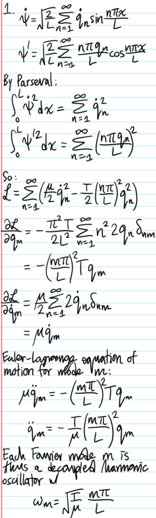
Problem: A string of length \(L\), mass per unit length \(\mu\), under uniform tension \(T\) is fixed at each end. The Lagrangian \(\mathcal L\) governing the time evolution of the transverse displacement \(\psi(x,t)\) is:
\[\mathcal L=\int_{0}^L\left(\frac{\mu}{2}\dot{\psi}^2-\frac{T}{2}\psi’^2\right)dx\]
where \(x\in[0,L]\) identifies position along the string from one endpoint. By expressing the transverse displacement as a Fourier sine series:
\[\psi(x,t)=\sqrt{\frac{2}{L}}\sum_{n=1}^{\infty}q_n(t)\sin\frac{n\pi x}{L}\]
Show that the Lagrangian \(\mathcal L\) becomes:
\[\mathcal L=\sum_{n=1}^{\infty}\left(\frac{\mu}{2}\dot{q}^2_n-\frac{T}{2}\left(\frac{n\pi}{L}\right)^2q_n^2\right)\]
Derive the equations of motion. Hence, show that the string is equivalent to an infinite set of decoupled harmonic oscillators with frequencies:
\[\omega_n=\sqrt{\frac{T}{\mu}}\frac{n\pi}{L}\]
Solution:
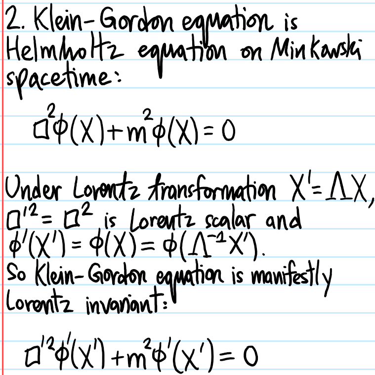
Problem: Show that the solution space of the Klein-Gordon equation is closed under Lorentz transformations.
Solution:
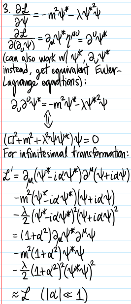
Problem: The motion of a complex scalar field \(\psi(X)\) is governed by the Lagrangian density:
\[\mathcal L=\partial_{\mu}\psi^*\partial^{\mu}\psi-m^2\psi^*\psi-\frac{\lambda}{2}(\psi^*\psi)^2\]
Write down the Euler-Lagrange field equations for this system. Verify that the Lagrangian density \(\mathcal L\) is invariant under the infinitesimal transformation:
\[\delta\psi=i\alpha\psi\]
\[\delta\psi^*=-i\alpha\psi^*\]
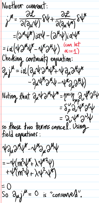
Derive the Noether current \(j^{\mu}\) associated with this transformation and verify explicitly that it is conserved using the field equations satisfied by \(\psi\).
Solution:
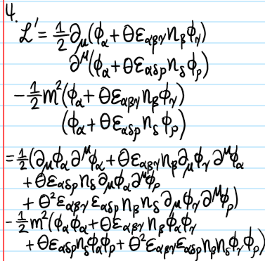
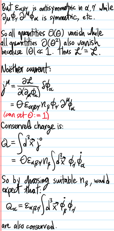
Problem: Verify that the Lagrangian density:
\[\mathcal L=\frac{1}{2}\partial_{\mu}\phi_{\alpha}\partial^{\mu}\phi_{\alpha}-\frac{1}{2}m^2\phi_{\alpha}\phi_{\alpha}\]
for a triplet of real fields \(\phi_{\alpha}(X)\), \(\alpha=1,2,3\), is invariant under the infinitesimal \(SO(3)\) rotation by \(\theta\):
\[\phi_{\alpha}\mapsto\phi_{\alpha}+\theta\varepsilon_{\alpha\beta\gamma}n_{\beta}\phi_{\gamma}\]
where \(n_{\beta}\) is a unit vector. Compute the Noether current \(j^{\mu}\) associated to this transformation. Deduce that the three quantities:
\[Q_{\alpha}=\int d^3\textbf x\varepsilon_{\alpha\beta\gamma}\dot{\phi}_{\beta}\phi_{\gamma}\]
are all conserved.
Solution:
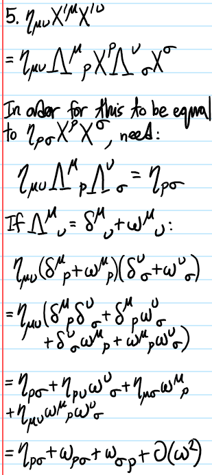
Problem: By requiring that Lorentz transformations \(\Lambda^{\mu}_{\space\space\nu}\) should preserve the Minkowski norm of \(4\)-vectors \(\eta_{\mu\nu}X’^{\mu}X’^{\nu}=\eta_{\mu\nu}X^{\mu}X^{\nu}\), show that this implies:
\[\eta_{\mu\nu}=\eta_{\sigma\tau}\Lambda^{\sigma}_{\space\space\mu}\Lambda^{\tau}_{\space\space\nu}\]
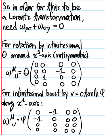
Show that an infinitesimal transformation of the form \(\Lambda^{\mu}_{\space\space\nu}=\delta^{\mu}_{\space\space\nu}+\omega^{\mu}_{\space\space\nu}\) is specifically a Lorentz transformation iff \(\omega_{\mu\nu}=-\omega_{\nu\mu}\) is antisymmetric.
Write down the matrix for \(\omega^{\mu}_{\space\space\nu}\) corresponding to an infinitesimal rotation by angle \(\theta\) around the \(x^3\)-axis. Do the same for an infinitesimal Lorentz boost along the \(x^1\)-axis by velocity \(v\).
Solution:
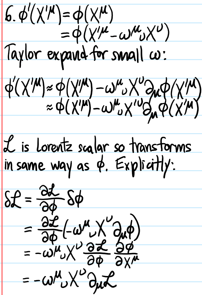
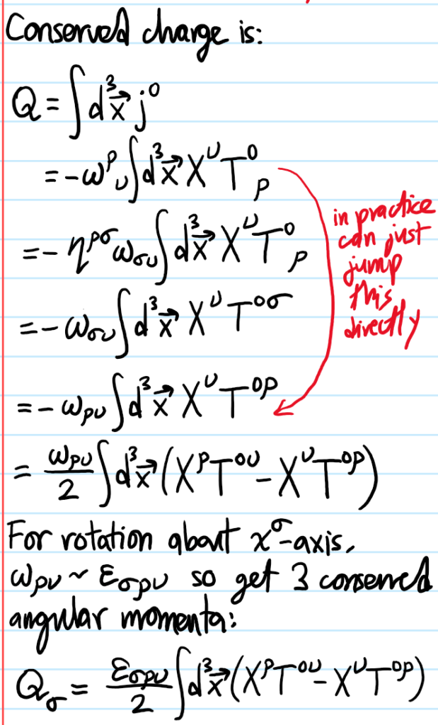
Problem: Consider a general infinitesimal Lorentz transformation \(X^{\mu}\mapsto X’^{\mu}=X^{\mu}+\omega^{\mu}_{\space\space\nu}X^{\nu}\) acting at the level of the \(4\)-vector \(X\). How does this perturbation manifest at the level of a scalar field \(\phi=\phi(X)\)? What about at the level of the Lagrangian density \(\mathcal L=\mathcal L(\phi)\)? What about at the level of the action \(S=S(\mathcal L)\)? In particular, show that the perturbation \(\delta\mathcal L\) at the level of \(\mathcal L\) is a total spacetime derivative, and hence describe the Noetherian implication of this.
Solution:
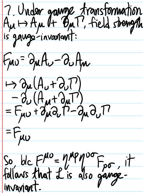
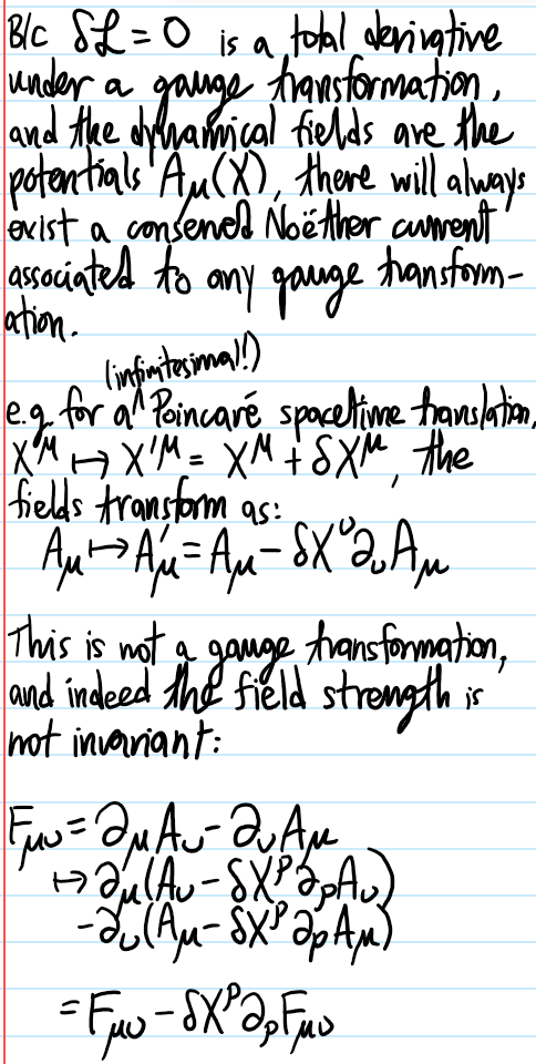
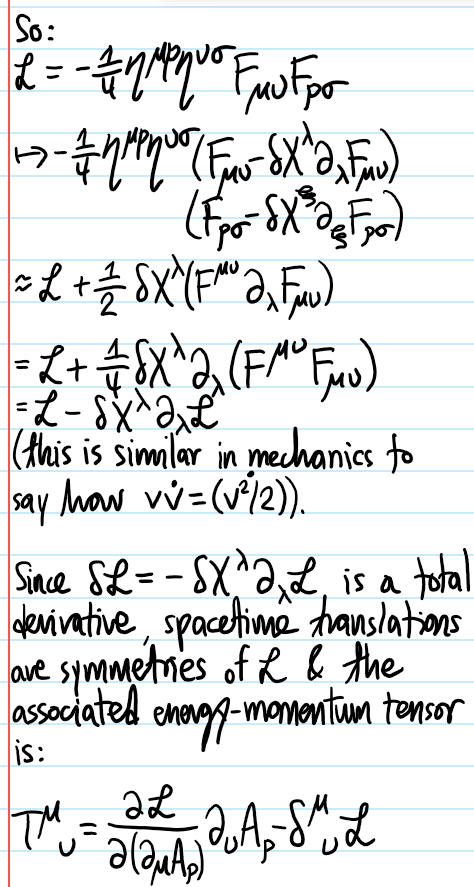
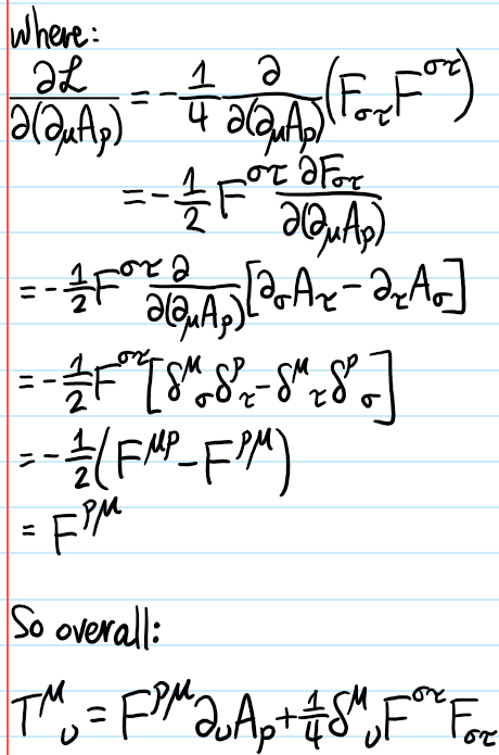
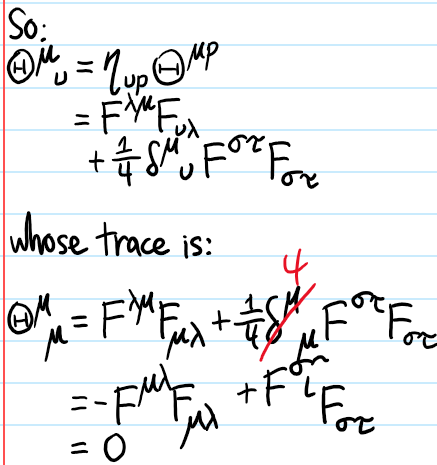
Problem: Maxwell’s Lagrangian for the electromagnetic field is:
\[\mathcal L=-\frac{1}{4}F_{\mu\nu}F^{\mu\nu}\]
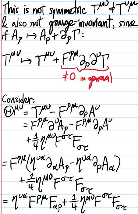
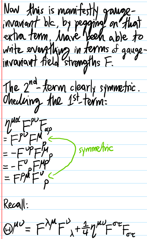
where \(F_{\mu\nu}=\partial_{\mu}A_{\nu}-\partial_{\nu}A_{\mu}\) and \(A_{\mu}\) is the \(4\)-vector potential. Show that \(\mathcal L\) is invariant under gauge transformations \(A_{\mu}\mapsto A_{\mu}+\partial_{\mu}\Gamma\) where \(\Gamma=\Gamma(X)\) is a scalar field with arbitrary (differentiable) dependence on \(X\). Use Noether’s theorem, and the spacetime translational invariance of the action \(S\) to construct the energy-momentum tensor \(T^{\mu\nu}\) for the electromagnetic field. Show that the resulting object is neither symmetric nor gauge invariant. Consider a new tensor given by:
\[\Theta^{\mu\nu}=T^{\mu\nu}-F^{\rho\mu}\partial_{\rho}A^{\nu}\]
Show that this object also defines \(4\) conserved currents. Moreover, show that it is symmetric, gauge invariant and traceless.
Solution:
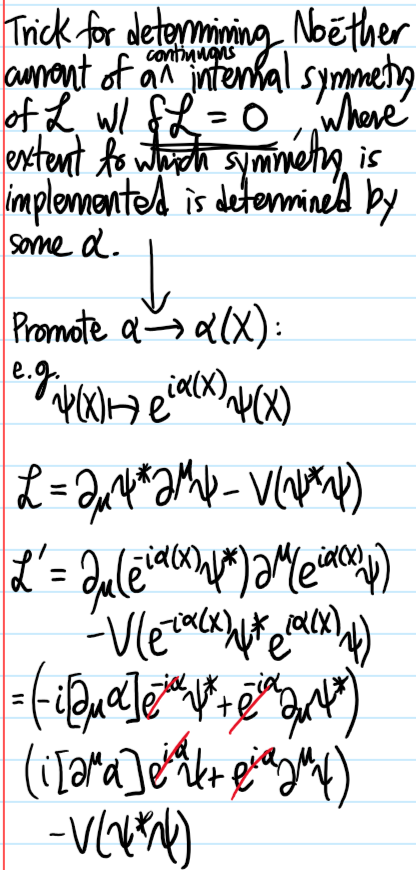
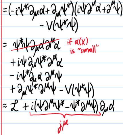
Problem: In Problem #\(3\), a classical field theory involving two complex scalar fields \(\psi(X),\psi^*(X)\) with Lagrangian density:
\[\mathcal L(\psi,\psi^*,\partial_{\mu}\psi,\partial_{\mu}\psi^*)=\partial_{\mu}\psi^*\partial^{\mu}\psi-V(\psi^*\psi)\]
was analyzed (there the potential \(V\) was taken to be analytic in \(\psi^*\psi\) and so Taylor expanded to quadratic order). In particular, the Noether current \(j^{\mu}\) was obtained explicitly for the continuous global, internal \(U(1)\) \(\mathcal L\)-symmetry \(\psi\mapsto e^{i\alpha}\psi\) for a constant \(\alpha\in\textbf R\). By promoting \(\alpha=\alpha(X)\) but still acting infinitesimally across \(X\) in spacetime, recompute the Noether current \(j^{\mu}\), and notice in particular that the Noether current \(j^{\mu}\) doesn’t care about the potential terms \(V(\psi^*\psi)\), only the kinetic terms.
Solution: