
The purpose of this post is to prove several general identities concerning the quantum statistical mechanics of an isolated, ideal Bose gas at equilibrium.
Problem #\(1\): Specify the physics (i.e. write down the Hamiltonian \(H\) for an isolated, ideal Bose gas).
Solution #\(1\): Because the Bose gas is isolated, there is no external potential \(V_{\text{ext}}=0\) and because it is ideal, there are no internal interactions \(V_{\text{int}}=0\). This leaves only the relativistic kinetic energy, and the single-boson Hamiltonian \(H\) is given by the usual dispersion relation:
\[H=\sqrt{\textbf P^2c^2+m^2c^4}-mc^2\]
However, for the typical case of nonrelativistic \(|\textbf P|\ll mc\) massive bosons, \(H\approx|\textbf P|^2/2m\), and for the less typical but still important case of (necessarily relativistic) massless \(m=0\) bosons (e.g. photons), \(H=|\textbf P|c\).
Problem #\(2\): By carefully considering what it means to be a boson, explain why one should work in the grand canonical ensemble.
Solution #\(2\): If \(\mathcal H\) denotes a single-boson state space, then the state space of \(N\) identical bosons is the \(N\)-fold symmetric tensor product \(S^N(\mathcal H)\subseteq\mathcal H^{\otimes N}\), i.e. two states \(|\Psi\rangle,|\Psi’\rangle\in S^N(\mathcal H)\) are physically equivalent \(|\Psi’\rangle\equiv|\Psi\rangle\) iff both specify exactly the same number of bosons \(N_{|\textbf k\rangle}\in\textbf N\) in each single-boson state \(|\textbf k\rangle\in\mathcal H\).
This means that, although experimentally \(N\) is typically fixed (massless \(m=0\) bosons like photons being the exception), mathematically any sum of the form \(\sum_{|\Psi\rangle\in S^N(\mathcal H)}\) for fixed \(N\) (which would arise when computing the partition function in the microcanonical or canonical ensembles) is a non-trivial combinatorics problem to parameterize. Thus, solely motivated by ease of mathematical calculation, one should allow the total number of bosons \(N\) in the Bose gas to fluctuate in diffusive equilibrium with an external particle bath \(\mu\), hence working in the grand canonical ensemble.
Problem #\(3\): Write down an expression for the grand canonical potential \(\Phi\), stating any assumptions.
Solution #\(3\): As usual, \(\Phi=-\beta^{-1}\ln\mathcal Z\), where the grand canonical partition function is:
\[\mathcal Z=\prod_{|\textbf k\rangle\in\mathcal H}\sum_{N_{|\textbf k\rangle}=0}^{\infty}e^{-\beta(N_{|\textbf k\rangle}E_{|\textbf k\rangle}-\mu N_{|\textbf k\rangle})}\]
where, from Solution #\(1\), the energy of the single-boson plane wave state is \(E_{|\textbf k\rangle}=\sqrt{\hbar^2|\textbf k|^2c^2+m^2c^4}-mc^2\). The geometric series converges for all \(|\textbf k\rangle\in\mathcal H\) iff \(\mu<E_{|\textbf k\rangle}\) for all \(|\textbf k\rangle\in\mathcal H\); since the kinetic energy is positive semi-definite (reaching its global minimum \(E_{|\textbf 0\rangle}=0\) for the \(\textbf k=\textbf 0\) ground state), this in turn is logically equivalent to the condition of a strictly negative chemical potential \(\mu<0\) (how to explain that this condition is violated for massless bosons and also for Bose-Einstein condensates, both of which have \(\mu=0\)? edit: one way I just thought of approaching this is to take Zoran’s perspective about the \(c\) subscript being placed on \(N_c\) rather than the experimentally more pertinent \(T_c\), i.e. recall the argument was that for a fixed \(T\), one can find an \(N_c\) such that if \(N=N_c\), then \(T=T_c\)…but then recalling \(T_c\propto N^{2/3}\) in a box trap or \(T_c\propto N^{1/3}\) in a harmonic trap, hence monotonically increasing functions of \(N\), so for \(N>N_c\), occupation of ground state is \(N-N_c\) (so in principle can get BEC at room temperature \(T\) just will need to surpass a ridiculous \(N_c\)). Hence:
\[\Phi=\beta^{-1}\sum_{|\textbf k\rangle\in\mathcal H}\ln\left(1-e^{-\beta(E_{|\textbf k\rangle}-\mu)}\right)\]
Problem #\(4\): Using Solution #\(3\), write down series for:
- The average pressure \(\langle p\rangle\)
- The entropy \(S\)
- The average boson number \(\langle N\rangle\) (and deduce the Bose-Einstein distribution)
- The average energy \(\langle E\rangle\)
Solution #\(4\):
\[p=-\frac{\Phi}{V}=-(\beta V)^{-1}\sum_{|\textbf k\rangle\in\mathcal H}\ln\left(1-e^{-\beta(E_{|\textbf k\rangle}-\mu)}\right)\]
\[S=-\frac{\partial\Phi}{\partial T}=\]
\[\langle N\rangle=-\frac{\partial\Phi}{\partial\mu}=\]
From which the Bose-Einstein distribution of Bose occupation numbers \(N_{|\textbf k\rangle}\) is:
\[N_{|\textbf k\rangle}=\frac{1}{e^{\beta(E_{|\textbf k\rangle-\mu})}-1}\]
\[\langle E\rangle=\frac{\partial(\Phi/\beta)}{\partial\beta}=\]
Problem #\(5\): Write down the relativistic density of states \(g(k)\). Hence compute \(g(E)\). What does it reduce to in the non-relativistic limit \(E\ll mc^2\) and in the massless \(m=0\) limit?
Solution #\(5\): Assuming infinite space periodic boundary conditions:
\[g(k)=\frac{\sigma V}{(2\pi)^3}4\pi k^2\]
where \(\sigma\) is some additional factor accounting for degrees of freedom besides \(\textbf k\) (e.g. \(\sigma=2\) for the polarization qubit of a photon). So:
\[g(E)=g(k)\frac{\partial k}{\partial E}=\frac{\sigma V}{2\pi^2\hbar^3c^3}(E+mc^2)\sqrt{(E+mc^2)^2-m^2c^4}\]
If \(E\ll mc^2\), this becomes approximately:
\[g(E)\approx \]
Problem #\(6\): Hence, using Solution #\(5\), estimate the excited state population \(N^*\) and corresponding excited kinetic energy \(E^*\). Explain why the ground state is not accounted for.
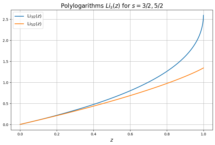
\[\Phi=-\frac{m^{3/2}V}{\sqrt{2}\pi^2\beta\hbar^3}\int_0^{\infty}\sqrt{E}\ln(1-ze^{-\beta E})dE=-\frac{V}{\beta\lambda^3}\text{Li}_{5/2}(z)\]
\[\langle N\rangle=\frac{m^{3/2}V}{\sqrt{2}\pi^2\hbar^3}\int_0^{\infty}\frac{\sqrt{E}}{z^{-1}e^{\beta E}-1}dE=\frac{V}{\lambda^3}\text{Li}_{3/2}(z)\]
\[\langle E\rangle=\frac{m^{3/2}V}{\sqrt{2}\pi^2\hbar^3}\int_0^{\infty}\frac{E^{3/2}}{z^{-1}e^{\beta E}-1}dE=\frac{3V}{2\beta\lambda^3}\text{Li}_{5/2}(z)\]
where \(z:=e^{\beta\mu}\in (0, 1)\) is called the fugacity of the ideal Bose gas, \(\lambda=\sqrt{\frac{2\pi\hbar^2}{mkT}}\) is the thermal de Broglie wavelength of the ideal Bose gas, and the polylogarithm is defined by the series \(\text{Li}_s(z):=\sum_{n=1}^{\infty}\frac{z^n}{n^s}\), so for instance \(\text{Li}_s(1)=\zeta(s)\) and \(\int_0^{\infty}\frac{x^{s-1}}{z^{-1}e^x-1}dx=\Gamma(s)\text{Li}_s(z)\).
Recalling that \(\Phi=-pV\) in the grand canonical ensemble, one therefore obtains (in an indirect form) the equation of state for an ideal Bose gas:
\[pV=\frac{2}{3}\langle E\rangle\]
Or, working in the thermodynamic limit henceforth:
\[pV=\frac{2}{3}E\]
At first, this looks exactly the same as the equation of state \(pV=NkT\) for just a classical (non-bosonic) ideal gas since there the kinetic energy is \(E=\frac{3}{2}NkT\). To see how in fact the equation of state for the ideal Bose gas is not the same as that of the ideal classical gas (i.e. that \(E\neq\frac{3}{2}NkT\) for the ideal Bose gas), clearly one must find how \(E=E(N,T)\) is related to \(N\) and \(T\). Conceptually this is straightforward since above one has already computed \(N=N(\mu, T)\) and \(E=E(\mu, T)\), so one just has to first invert \(N=N(\mu,T)\) in the form \(\mu=\mu(N,T)\) and then substitute this into \(E=E(\mu,T)=E(\mu(N,T),T)=E(N,T)\) which can be plugged into the equation of state to obtain \(pV=\frac{2}{3}E(N,T)\). Practically, there is no simple analytical way to do this for arbitrary temperatures \(T\) and chemical potential \(\mu\).
Instead, the next best thing one can hope for is to get a sense of the physics at the two extremes of the fugacity \(z\in(0,1)\), namely the high-temperature limit \(z\to 0\) and the low-temperature limit \(z\to 1\) (it is a priori counterintuitive that \(z\to 0\) is a high-\(T\) expansion or that \(z\to 1\) is a low-\(T\) expansion considering \(\mu<0\); this only becomes apparent a posteriori). In the high-\(T\) case \(z\to 0\), some algebra gives the second-order virial expansion for the high-temperature equation of state of an ideal Bose gas:
\[pV=NkT\left(1-\frac{\lambda^3N}{4\sqrt{2}V}+O\left(\frac{N}{V}\right)^2\right)\]
Thus, compared to an ideal gas at the same temperature \(T\), the effect of bosonic statistics is to reduce the pressure \(p\) a little bit, but otherwise, at high temperatures \(T\to\infty\), the ideal Bose gas and ideal classical gas are basically the same.
The more interesting physics lurks in the low-\(T\) limit \(z\to 1\). In this case, it is clear that the number of bosons in the ideal Bose gas approaches:
\[N\to\frac{\zeta(3/2)V}{\lambda^3_c}\]
at a critical temperature \(T_c\) given by:
\[T_c=\frac{2\pi\hbar^2}{mk}\left(\frac{N}{\zeta(3/2)V}\right)^{2/3}\]
However, suppose one were to cool below the critical temperature \(T<T_c\). Supposing that \(z\) remains capped at \(1\) (otherwise the polylogarithm \(\text{Li}_{3/2}(z)\) would diverge for \(z>1\) as the graph suggests), then because \(\lambda\propto T^{-1/2}\), this implies that the number of bosons \(N\) should decrease, but that is absurd because \(V\) is constant and the number of bosons \(N\) does not fluctuate enough in the thermodynamic limit \(\sigma_N/N\sim N^{-1/2}\) to explain this decrease. The resolution to this paradox is subtle and cuts to the heart of Bose-Einstein condensation. Recall from the Bose-Einstein distribution that the Bose occupation number \(N_0=\langle N_0\rangle\) of the single-boson ground state \(|0\rangle\) (whose energy is \(E_0=0\)) is:
\[N_0=\frac{1}{z^{-1}-1}\]
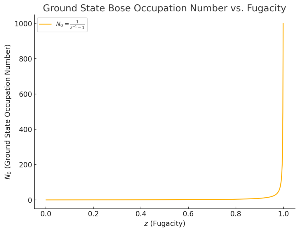
So more and more bosons in the ideal Bose gas will, in the low-temperature limit \(z\to 1\), condense into the ground state \(|0\rangle\) as evidenced by the blowup of \(N_0\) at \(z=1\). However, earlier the replacement \(\sum_{|k\rangle\in\mathcal H_0}\mapsto\int_0^{\infty}g(E)dE\) when evaluating the average number of bosons \(\langle N\rangle\) would have (in this \(z\to 1\) edge case) undercounted all of these bosons condensing in the ground state \(|0\rangle\) because the density of states \(g(E)\propto\sqrt{E}\) vanishes \(g(0)=0\) at the ground state energy \(E_0=0\). Instead, one can just manually add \(N_0=(z^{-1}-1)^{-1}\) into the total boson count “by hand” to obtain the revised count:
\[N=\frac{V}{\lambda^3}\text{Li}_{3/2}(z)+\frac{1}{z^{-1}-1}\]
The way to read this is that the first term \(\frac{V}{\lambda^3}\text{Li}_{3/2}(z)\) is the total number of bosons not in the ground state, which as \(z\to 1\) should become negligible in comparison to the Bose occupation number \(N_0\) of the ground state. In this limit, one has:
\[N\to\frac{1}{z^{-1}-1}\Rightarrow z\to\left(1+\frac{1}{N}\right)^{-1}\approx 1-\frac{1}{N}<1\]
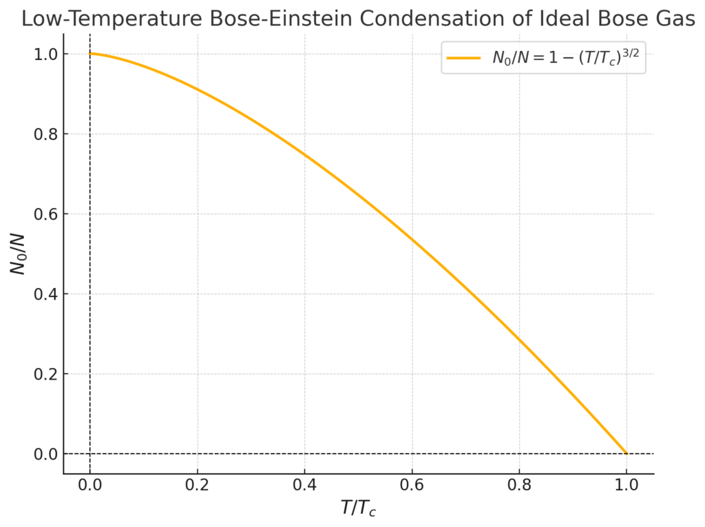
So the fugacity \(z\) is naturally capped by however many bosons \(N\) one started with, regardless of how low the temperature \(T\to 0\) drops. More precisely, as \(T<T_c\) drops below the critical temperature, the fraction \(N_0/N\) of bosons in the ground state \(|0\rangle\) grows monotonically towards \(N_0/N\to 1\) as \(T/T_c\to 0\) in the manner:
\[\frac{N_0}{N}=\frac{1}{1+(N-N_0)/N_0}\approx 1-\frac{N-N_0}{N_0}\approx 1-\frac{\zeta(3/2)V}{N\lambda^3_c}=1-\left(\frac{T}{T_c}\right)^{3/2}\]
This low-temperature bosonic communism is called Bose-Einstein condensation.
As for the low-temperature \(T<T_c\) equation of state for the ideal Bose gas, one has the previous grand canonical potential but with an additional contribution from the BEC in the ground state:
\[\Phi=-\frac{V}{\beta\lambda^3}\text{Li}_{5/2}(z)+\frac{1}{\beta}\ln(1-z)\]
As \(z\to 1-\frac{1}{N}\) maxes out:
\[\Phi\to -\frac{1}{\beta}\left(\frac{\zeta(5/2)V}{\lambda^3}+\ln N\right)\]
However, this makes it clear that, unlike for the total boson number \(N\), here the ground state contribution to the grand canonical potential \(\Phi\) is actually negligible in the thermodynamic limit because \(V/\lambda^3\sim N\) is much larger than \(\ln(N)\). The low-\(T\) equation of state for the ideal Bose gas (well actually now the BEC) is therefore:
\[p=\frac{\zeta(5/2)}{\beta\lambda^3}\sim T^{5/2}\]
Clearly, this is now very different from the classical ideal gas. Notably, the pressure \(p\) is independent of the bosonic number density \(N/V\), the intuition being that the vast number of bosons condensing in the motional ground state \(|k\rangle=|0\rangle\) will be (roughly) frozen in place and therefore make negligible contribution to the pressure \(p\).
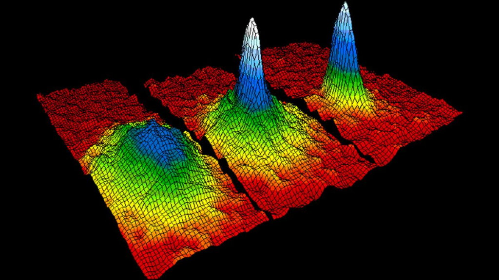
For now, there is one more interesting thing to mention about Bose-Einstein condensation; clearly it’s a phase transition between two radically different states of matter, namely from a(n ideal Bose) gas to a BEC (cf. gaseous steam \(\text H_2\text O(g)\) condensing into liquid water \(\text H_2\text O(\ell)\)). Usually phase transitions are associated with some kind of discontinuity in physical properties at the phase transition; how does this manifest in the case of Bose-Einstein condensation at the critical temperature \(T=T_c\)? It turns out that the derivative \(\frac{\partial C_V}{\partial T}\) of the isochoric heat capacity \(C_V\) with respect to the temperature \(T\) is discontinuous at the critical temperature \(T=T_c\) (although the heat capacity \(C_V=C_V(T)\) itself is continuous). This is reminiscent (and related to) the superfluid \(\lambda\)-transition seen in bosonic \(^4\text{He}\) at \(T\approx 2.17\text{ K}\).