
Problem: Given a system of \(N\) identical bosons or fermions with Hamiltonian \(H\) in a mixed ensemble described by a density operator \(\rho\) (usually \(\rho=e^{-\beta H}/Z\) or \(\rho=e^{-\beta(H-\mu N)}/Z\) in equilibrium at temperature \(T=1/k_B\beta\) and chemical potential \(\mu\) though one can also work with a non-equilibrium \(\rho\); another limit often taken is \(T=0\) in which case the system is guaranteed to be in its ground state) and two operators \(P(t),Q(t)\) in the Heisenberg picture, define the greater Green’s function \(G^{>}_{P,Q}(t,t’)\), the lesser Green’s function \(G^{<}_{P,Q}(t,t’)\), the causal Green’s function \(G_{P,Q}(t,t’)\), the retarded Green’s function \(G^+_{P,Q}(t,t’)\), and the advanced Green’s function \(G^-_{P,Q}(t,t’)\) of \(P\) and \(Q\).
Solution: In all the formulas, the expectation is with respect to \(\rho\), (\(\langle A\rangle=\text{Tr}(\rho A)\) which at \(T=0\) looks like typical QFT expectations \(\langle \space|A|\space\rangle\) in a vacuum ground state \(|\space\rangle\)), and in all \(\pm,\mp\) occurrences, the “top” sign is for bosons while the “bottom” sign is for fermions:
\[G^{>}_{P,Q}(t,t’)=-\frac{i}{\hbar}\langle P(t)Q(t’)\rangle\]
\[G^{<}_{P,Q}(t,t’)=\mp\frac{i}{\hbar}\langle Q(t’)P(t)\rangle\]
\[G_{P,Q}(t,t’)=\Theta(t-t’)G^{>}_{P,Q}(t,t’)+\Theta(t’-t)G^{<}_{P,Q}(t,t’)=-\frac{i}{\hbar}\langle\mathcal T P(t)Q(t’)\rangle\]
(note that \(\mathcal T P(t)Q(t’)=\Theta(t-t’)P(t)Q(t’)\pm\Theta(t’-t)Q(t’)P(t)\) and in particular for fermions the time-ordering is not simply equal to \(\mathcal T P(t)Q(t’)\neq \Theta(t-t’)P(t)Q(t’)+\Theta(t’-t)Q(t’)P(t)\))
\[G^{\pm}_{P,Q}(t,t’)=\pm\Theta(\pm(t-t’))(G^{>}_{P,Q}(t,t’)-G^{<}_{P,Q}(t,t’))=\mp\frac{i}{\hbar}\Theta(\pm(t-t’))\langle [P(t),Q(t’)]_{\mp}\rangle\]
where \([A,B]_{-}=[A,B]\) is the commutator for bosons while \([A,B]_-=\{A,B\}\) is the anticommutator for fermions, i.e. \([A,B]_{\pm}=AB\pm BA\).
(comment about if \(H=H_0+V\) and using interaction picture instead of Heisenberg).
Problem: Show that if the Hamiltonian \(H\) is time-independent and the density operator \(\rho=\rho(H)\) is a function of \(H\) only (such as in equilibrium \(\rho=e^{-\beta H}/Z\)), then all \(5\) Green’s functions are a function of only the time difference \(t-t’\).
Solution: Clearly it suffices to show it for the greater and lesser Green’s functions. Specifically, for any \(2\) Heisenberg operators \(P(t),Q(t’)\), one has:
\[\langle P(t)Q(t’)\rangle=\frac{1}{Z}\text{Tr}\left(\rho P(t)Q(t’)\right)\]
Since \(H\) is time-independent, the time-evolution operator is just \(e^{-iHt/\hbar}\) and hence the Heisenberg operators are \(P(t)=e^{iHt/\hbar}Pe^{-iHt/\hbar}\) and \(Q(t’)=e^{iHt’/\hbar}Qe^{-iHt’/\hbar}\) so:
\[=\frac{1}{Z}\text{Tr}\left(\rho e^{iHt/\hbar}Pe^{-iH(t-t’)/\hbar}Qe^{-iHt’/\hbar}\right)\]
but by cyclicity of the trace and the fact that \(\rho\) is a function of \(H\), and so commutes with any other function of \(H\):
\[=\frac{1}{Z}\text{Tr}\left(\rho e^{iH(t-t’)/\hbar}Pe^{-iH(t-t’)/\hbar}Q\right)\]
and the claim follows. Thus, in such cases there is no harm in letting \(t’:=0\).
Problem: For single-particle Green’s functions, what are \(P(t)\) and \(Q(t)\) typically? What about for two-particle Green’s functions (and beyond)?
Solution: For single-particle Green’s functions (called such even though it’s really still a many-body object because it’s sensitive to the full Hamiltonian \(H\)), the standard case of interest is \(P(t)=c_i(t)\) and \(Q(t’):=c^{\dagger}_j(t’)\) where \(\{|i\rangle\}\) is a basis of the single-particle state space and \(c_i, c^{\dagger}_j\) are the annihilation and creation operators associated to \(|i\rangle\) and \(|j\rangle\) respectively. For example, if one is dealing with a bunch of electrons moving in \(\mathbf R^3\) and one chooses \(|i\rangle\equiv |\mathbf x,\sigma\rangle\), then the single-particle retarded Green’s function (thought of as a \(2\times 2\) matrix) can be written as:
\[G^+_{\sigma\sigma’}(\mathbf x,t;\mathbf x’,t’)=-\frac{i}{\hbar}\Theta(t-t’)\langle\{\psi_{\sigma}(\mathbf x,t),\psi^{\dagger}_{\sigma’}(\mathbf x’,t’)\}\rangle\]
Alternatively, picking \(|i\rangle\equiv |\mathbf k,\sigma\rangle\) leads to:
\[G^+_{\mathbf k\sigma,\mathbf k’\sigma’}(t,t’)=-\frac{i}{\hbar}\Theta(t-t’)\langle\{c_{\mathbf k\sigma}(t),c^{\dagger}_{\mathbf k’\sigma’}(t’)\}\rangle\]
Single-particle Green’s functions are also loosely referred to as two-point correlation functions. By extension, an example of a two-particle Green’s function might take \(P(t)=N_{\mathbf k}(t):=\sum_{\mathbf k’\sigma}c_{\mathbf k’+\mathbf k,\sigma}(t)c_{\mathbf k’\sigma}(t)\) and \(Q(t’)=N_{-\mathbf k}(t’)\) which would be a four-point correlation function.
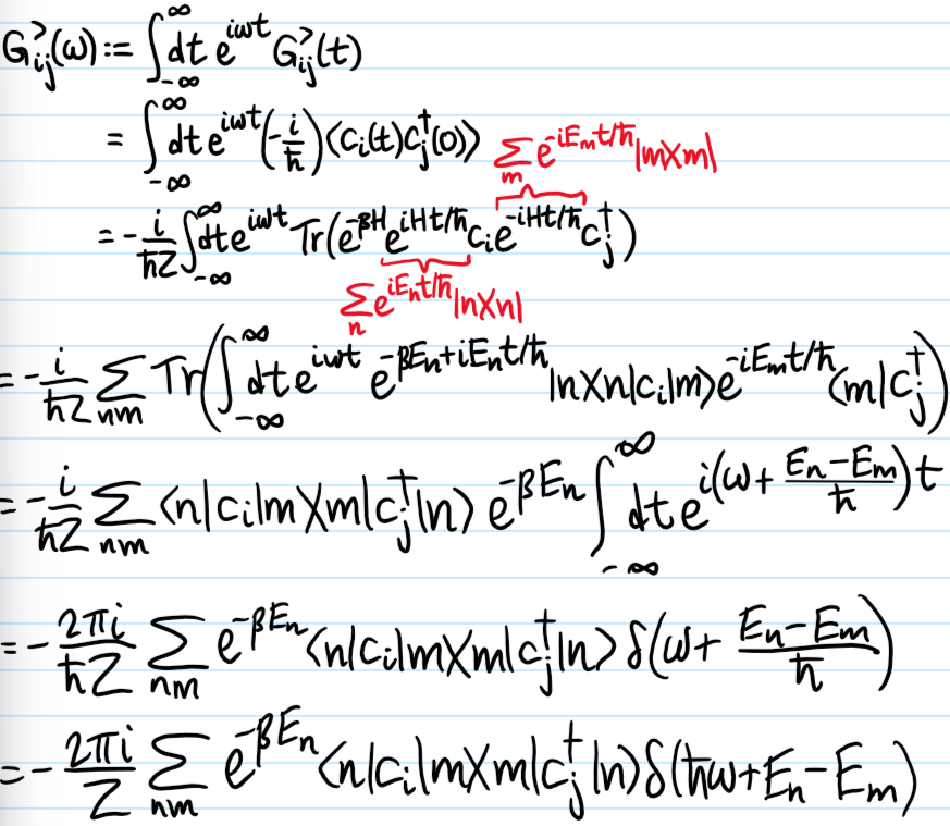
Problem: As mentioned earlier, when \(\rho=e^{-\beta H}/Z\) and \(\dot H=0\), one can set \(t’:=0\) without loss of information. In this case, being left with only a single time variable \(t\), one can Fourier transform each of the \(5\) single-particle Green’s functions from the time domain \(t\mapsto\omega\) to the frequency domain (with the usual linear response convention). In this case, show that the frequency-domain Green’s functions admit the Lehmann (also called spectral) representations:
\[G^{>}_{P,Q}(\omega)=-\frac{2\pi i}{Z}\sum_{nm}e^{-\beta E_n}\langle n|P|m\rangle\langle m|Q|n\rangle\delta(\hbar \omega+E_n-E_m)\]
\[G^{<}_{P,Q}(\omega)=\pm e^{-\beta\hbar\omega}G^{>}_{P,Q}(\omega)\]
\[G^+_{P,Q}(\omega)=\frac{1}{Z}\sum_{nm}\frac{\langle n|P|m\rangle\langle m|Q|n\rangle}{\hbar(\omega+i0^+)+E_n-E_m}(e^{-\beta E_n}\mp e^{-\beta E_m})\]
\[G^-_{P,Q}(\omega)=(G^+_{Q,P}(\omega))^*\]
where \(\{|n\rangle\}\) is an orthonormal \(H\)-eigenbasis.
Solution: (here the derivation was done with \(P=c_i\) and \(Q=c^{\dagger}_j\) but it works with arbitrary \(P,Q\)):

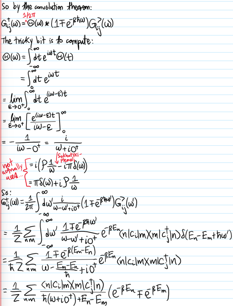
Problem: For each of the \(5\) frequency-domain Green’s functions (equilibrium \(\rho=e^{-\beta H}/Z\), time-independent \(H\) as before), one can define a corresponding spectral function. For instance, associated to the retarded Green’s function \(G_{P,Q}^+(\omega)\) is the retarded spectral function:
\[A^+_{P,Q}(\omega):=-2\hbar\text{Im}G_{P,Q}^+(\omega)\]
Show that, in the special but important case where \(Q=P^{\dagger}\), the corresponding retarded spectral function \(A^+_{P,P^{\dagger}}(\omega)\) scales with both the greater Green’s function \(G^>_{P,P^{\dagger}}(\omega)\) and the lesser Green’s function \(G^<_{P,P^{\dagger}}(\omega)\) in the frequency domain as:
\[A^+_{P,P^{\dagger}}(\omega)=i\hbar (1\mp e^{-\beta\hbar\omega})G^>_{P,P^{\dagger}}(\omega)=i\hbar (\mp e^{\beta\hbar\omega}-1)G^<_{P,P^{\dagger}}(\omega)\]
Or inverting:
\[i\hbar G^>_{P,P^{\dagger}}(\omega)=(1\pm N_{\mp}(\omega))A^+_{P,P^{\dagger}}(\omega)\]
\[\pm i\hbar G^<_{P,P^{\dagger}}(\omega)=N_{\mp}(\omega)A^+_{P,P^{\dagger}}(\omega)\]
where \(N_{\pm}(\omega):=\frac{1}{e^{\beta\hbar\omega}\pm 1}\) are respectively Bose-Einstein/Fermi-Dirac distributions. These relations go by the name of the fluctuation-dissipation theorem (valid at equilibrium!) because \(G^>\) and \(G^<\) are clearly a measure of fluctuations whereas the spectral function \(A^+\) measures dissipation by virtue of being \(\propto G^+\).
Solution: The quick and dirty way is to just use the Lehmann representation of \(G^+_{P,P^{\dagger}}(\omega)\), and when taking its imaginary part one just needs to invoke Sokhotski-Plemelj to get a bunch of \(\delta\)’s which makes it look very similar to the Lehmann representations of \(G^>_{P,P^{\dagger}}(\omega)\) and \(G^<_{P,P^{\dagger}}(\omega)\) from which the results follow.
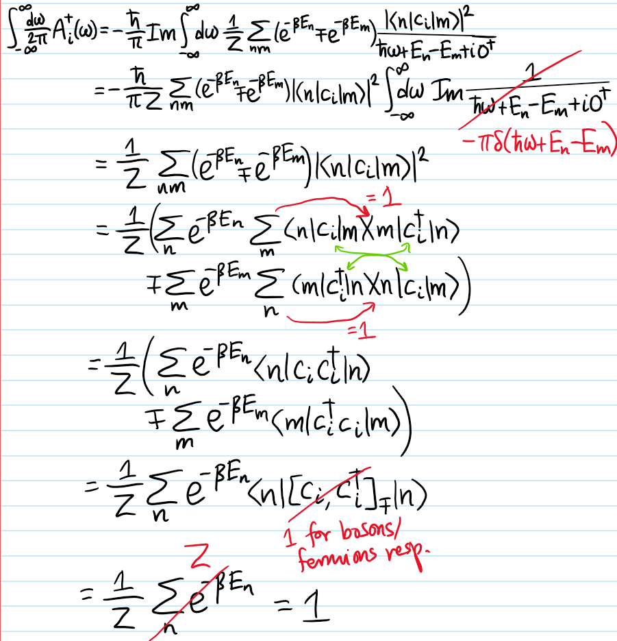
Problem: Specializing from the above problem, work with a diagonal component \(P=c_i\) of the single-particle retarded Green’s function. In this case, show that the retarded spectral function \(A^+_i(\omega)\) obeys the sum rule:
\[\int_{-\infty}^{\infty}\frac{d\omega}{2\pi}A^+_i(\omega)=1\]
Solution: This is the first time that the commutation/anticommutation relation is actually necessary:
(note: in some literature, the spectral function is taken to be \(A^+_{P,Q}(\omega)=-\frac{\hbar}{\pi}\text{Im}G^+_{P,Q}(\omega)\) such that with this convention the sum rule reads \(\int_{-\infty}^{\infty}d\omega A^+_{P,Q}(\omega)=1\)).
Connect these to the resolvent of \(H\) and FT of time-evolution operator? (see the Oxford text for more)
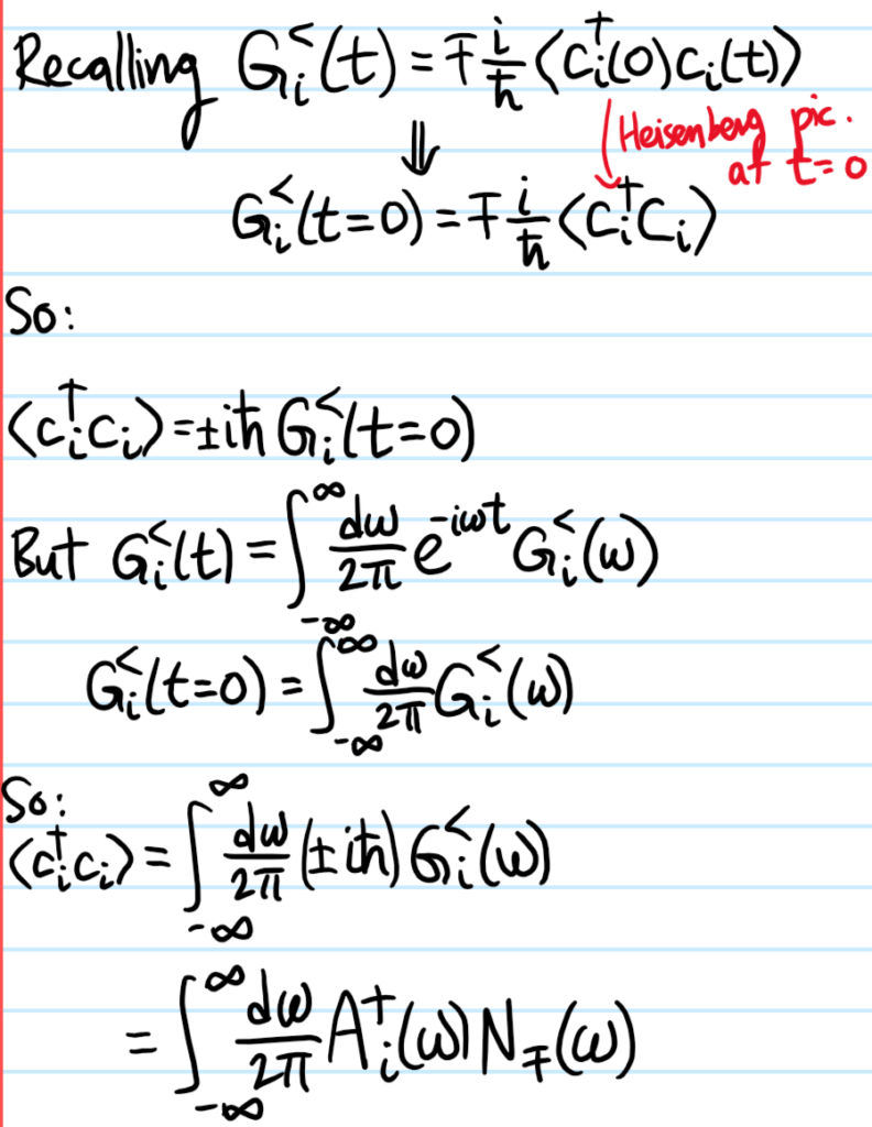
Problem: Show that the retarded spectral function \(A^+_i(\omega)\) behaves like a density of states:
\[\langle c^{\dagger}_ic_i\rangle=\int_{-\infty}^{\infty}\frac{d\omega}{2\pi}A_i^+(\omega)N_{\mp}(\omega)\]
Solution: Using hopefully obvious notation:
Problem: For a system of non-interacting identical bosons/fermions, what is the (retarded) spectral function \(A^+_{\sigma}(\mathbf k,\omega)\)?
Solution: In that case, \(H=\sum_{\mathbf k\sigma}\frac{\hbar^2|\mathbf k|^2}{2m}c^{\dagger}_{\mathbf k\sigma}c_{\mathbf k\sigma}\). Although one can directly use the Lehmann representation formulas given that for both bosons and fermions the eigenstates \(|n\rangle\) and spectrum \(E_n\) of \(H\) are well-understood, it’s instructive to do a “first-principles” derivation. Specifically, first one needs to show that the the free time evolution of the creation and annihilation operators is explicitly given by:
\[c_{\mathbf k\sigma}(t)=e^{-i\hbar|\mathbf k|^2t/2m}c_{\mathbf k\sigma}\]
\[c^{\dagger}_{\mathbf k\sigma}(t)=e^{i\hbar|\mathbf k|^2t/2m}c^{\dagger}_{\mathbf k\sigma}\]
The rigorous way is to simply downgrade from \(c_{\mathbf k\sigma}(t)=e^{iHt/\hbar}c_{\mathbf k\sigma}e^{-iHt/\hbar}\) back to the Heisenberg equation of motion \(i\hbar\dot c_{\mathbf k\sigma}(t)=[c_{\mathbf k\sigma}(t),H]=e^{iHt/\hbar}[c_{\mathbf k\sigma},H]e^{-iHt/\hbar}\) and upon inserting \(H=\sum_{\mathbf k’\sigma’}\frac{\hbar^2|\mathbf k’|^2}{2m}c^{\dagger}_{\mathbf k’\sigma’}c_{\mathbf k’\sigma’}\), recognize this as the commutator \([c_i,N_j]=\delta_{ij}c_i\) valid for both bosons and fermions (read it as a fancy way of saying \(N-(N-1)=1\)). This gives a \(1^{\text{st}}\)-order ODE for \(c_{\mathbf k\sigma}(t)\) with the trivial solution \(c_{\mathbf k\sigma}(t)=e^{-i\hbar |\mathbf k|^2t/2m}c_{\mathbf k\sigma}\), and by taking the adjoint one also gets \(c^{\dagger}_{\mathbf k\sigma}(t)=e^{-i\hbar |\mathbf k|^2t/2m}c^{\dagger}_{\mathbf k\sigma}\). The quicker, but more intuitively appealing way, is to directly take \(c_{\mathbf k\sigma}(t)=e^{iHt/\hbar}c_{\mathbf k\sigma}e^{-iHt/\hbar}\) and act on an arbitrary Fock state. The result then amounts to an identity of the form \(e^{i(E-\hbar^2|\mathbf k|^2/2m)t/\hbar}e^{-iEt/\hbar}=e^{-i\hbar|\mathbf k|^2t/2m}\). Armed with this, the diagonal retarded single-particle Green’s function is:
\[G^+_{\sigma}(\mathbf k,t)=-\frac{i}{\hbar}\Theta(t)\langle[c_{\mathbf k\sigma}(t),c^{\dagger}_{\mathbf k\sigma}]_{\mp}\rangle\]
\[=-\frac{i}{\hbar}\Theta(t)e^{-i\hbar |\mathbf k|^2 t/2m}\langle[c_{\mathbf k\sigma},c^{\dagger}_{\mathbf k\sigma}]_{\mp}\rangle\]
\[=-\frac{i}{\hbar}\Theta(t)e^{-i\hbar |\mathbf k|^2 t/2m}\]
by virtue of the CCR/CAR. With the help of an \(i\varepsilon\) prescription, this is easy to Fourier transform:
\[G^+_{\sigma}(\mathbf k,\omega)=-\frac{i}{\hbar}\int_0^{\infty}e^{i(\omega-\hbar|\mathbf k|^2/2m)t-\varepsilon t}\]
\[=\frac{1}{\hbar\omega-\frac{\hbar^2|\mathbf k|^2}{2m}+i0^+}\]
So finally, using the Sokhotski-Plemelj theorem:
\[A^+_{\sigma}(\mathbf k,\omega)=2\pi\delta\left(\omega-\frac{\hbar|\mathbf k|^2}{2m}\right)\]
which clearly fulfills the sum rule. As another corollary, applying the earlier result to this non-interacting system, one has:
\[\langle c^{\dagger}_{\mathbf k\sigma}c_{\mathbf k\sigma}\rangle=\int_{-\infty}^{\infty}\frac{d\omega}{2\pi}2\pi\delta\left(\omega-\frac{\hbar|\mathbf k|^2}{2m}\right)N_{\mp}(\omega)=N_{\mp}\left(\frac{\hbar|\mathbf k|^2}{2m}\right)=\frac{1}{e^{\beta\hbar^2|\mathbf k|^2/2m}\mp 1}\]
which reinforces that the Bose-Einstein/Fermi-Dirac distributions are strictly only valid for non-interacting systems of bosons/fermions.
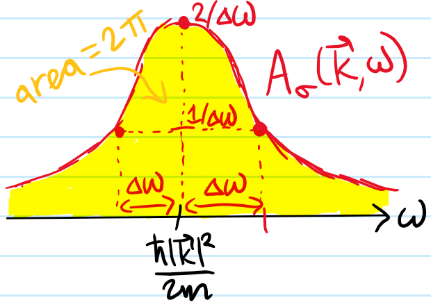
Problem: Above, the \(\varepsilon\)-prescription seemed to be a bit artificial…on the other hand, if one replaces \(\varepsilon\mapsto\Delta\omega\) so that the retarded Green’s function decays exponentially in time (due to interactions which scatter particles out of the state \(|\mathbf k\sigma\rangle\)) with non-infinitesimal decay rate \(\Delta\omega>0\), then show that the spectral function is broadened from a \(\delta\) spike into a Lorentzian with HWHM \(\Delta\omega\):
\[A^+_{\sigma}(\mathbf k,\omega)=\frac{2\Delta\omega}{(\omega-\hbar|\mathbf k|^2/2m)^2+\Delta\omega^2}\]
Solution: The diagonal single-particle retarded Green’s function is a Mobius transformation of \(\omega\):
\[G^+_{\sigma}(\mathbf k,\omega)=\frac{1}{\hbar\omega-\hbar^2|\mathbf k|^2/2m+i\hbar\Delta\omega}\]
and the claim follows. Aside: if \(\Delta\omega\) is not too large, then this gives rise to the idea of a quasiparticle from Landau’s Fermi liquid theory. In that case, a generic spectral function might have the form:
\[A^+_{\sigma}(\mathbf k,\omega)=\frac{2Z_{\mathbf k}\Delta\omega_{\mathbf k}}{(\omega-\hbar|\mathbf k|^2/2m)^2+\Delta\omega_{\mathbf k}^2}+\tilde A^+_{\sigma}(\mathbf k,\omega)\]
where \(Z_{\mathbf k}\in[0,1]\) is a momentum-dependent quasiparticle residue and in particular if \(Z_{\mathbf k}\neq 1\) then an incoherent background/continuum spectrum \(\tilde A^+_{\sigma}(\mathbf k,\omega)\) must be present in order for \(A^+_{\sigma}(\mathbf k,\omega)\) to still obey the sum rule.
Problem: Annotate the following Nature Physics paper.
Solution:
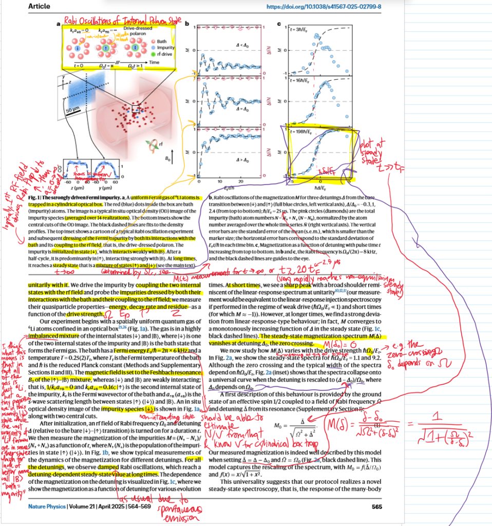
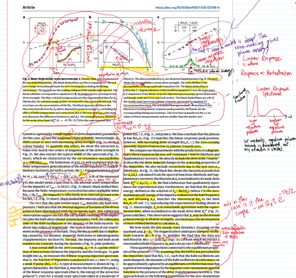
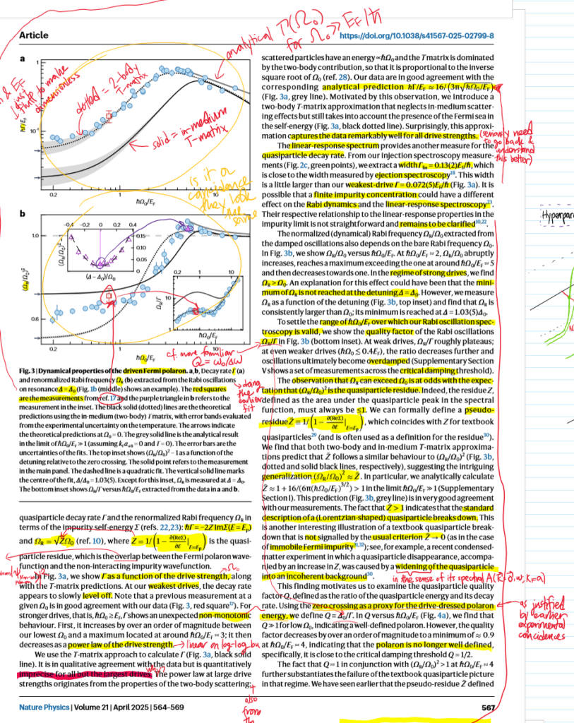
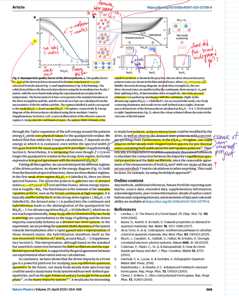
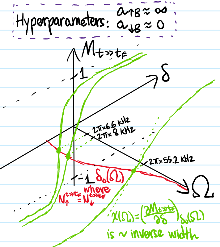
Everything in the first half of the paper (steady state part) can be summed up like:
And the latter half discussing the resonant dynamics of the pre-steady state can be visualized qualitatively as:
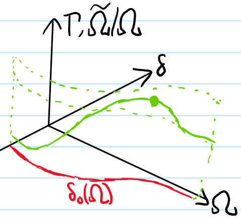
Finally, a few points worth emphasizing:
- Clearly \(\uparrow\) is unstable, wants to decay back to \(\downarrow\) with transition rate \(\Gamma\), so the zero-detuning \(\delta_0<0\) must contain information about the \(\uparrow,B\) interactions.
- A Rabi experiment is different from say Ramsey in that it really is about a continuous drive so \(t\gg 1/\Omega\), as mentioned in the paper’s Figure \(1a\).
- To emphasize again, there is the implicit hyperparameters that \(a_{\uparrow B}=\infty\) is unitarily/strongly interacting while \(a_{\downarrow B}\approx 0\) is weakly/non-interacting; the paper gives exact values). So only the attractive polaron is present. At the end the paper mentions extending into the BEC regime, where both would coexist for a sufficiently broad Feshbach resonance.
And some random thoughts I have about the paper:
- Instead of the \(3D\) surface graph, maybe a heat map would be instructive too?
- At large \(\Omega\), how does the AC Stark shift associated with a dressed atom-photon affect the physics (since it seems it would affect the internal energies of the polaron)?
Problem: Write an essay that summarizes the key points learned from the following papers/slides:
- Fermi polarons and beyond (Parish and Levinsen)
- The quantum impurity problem and beyond (Parish)
- Exact theory of the finite-temperature spectral function of Fermi polarons with multiple particle-hole excitations: Diagrammatic theory versus Chevy ansatz (Hu, Wang, Liu)
- A single impurity in an ideal atomic Fermi gas: current understanding and some open problems (Lan, Lobo)
- Many-particle physics with ultracold gases (Punk)
- Polarons, dressed molecules, and itinerant ferromagnetism in ultracold Fermi gases (Massignan, Zaccanti, Bruun)
- Ultrafast many-body interferometry of impurities coupled to a Fermi sea (Cetina et al.)
- https://static-content.springer.com/esm/art%3A10.1038%2Fs41567-025-02799-8/MediaObjects/41567_2025_2799_MOESM1_ESM.pdf
- file:///C:/Users/weidu/Downloads/Double_Mode_in_Driven_Fermi_Polaron.pdf
Solution: For a generic \(2\)-component Fermi gas whose \(2\) components may be called \(\uparrow\) and \(\downarrow\) (this could be \(2\) hyperfine states of the same atom, or \(2\) hyperfine states of different atoms) the Hamiltonian is \(H=H_0+V_{\downarrow\uparrow}\) where the kinetic energy is:
\[H_0=\sum_{\textbf k}\frac{\hbar^2|\textbf k|^2}{2m_{\uparrow}}c^{\dagger}_{\textbf k\uparrow}c_{\textbf k\uparrow}+\frac{\hbar^2|\textbf k|^2}{2m_{\downarrow}}c^{\dagger}_{\textbf k\downarrow}c_{\textbf k\downarrow}\]
and the short-range scattering pseudopotential \(V_{\downarrow\uparrow}\) of “bare strength” \(g_{\uparrow\downarrow}\) describes momentum-conserving collisions between the \(2\) components \(\uparrow,\downarrow\) of the Fermi gas in a volume \(V\) (note that interactions among the components themselves are neglected, i.e. they are separately ideal Fermi gases. That is, one assumes there is no \(\uparrow\uparrow\) or \(\downarrow\downarrow\) scattering. This is justified by the fact that identical spin parts of \(2\) identical fermions could only interact via an odd-\(\ell\) scattering channel, the lowest of which is \(\ell=1\) \(\p\)-wave scattering whose cross-section \(\sigma_{\ell}\sim k^{2\ell}\) is suppressed at low \(k\)):
\[V_{\downarrow\uparrow}=\frac{g_{\uparrow\downarrow}}{V}\sum_{\textbf k_1,\textbf k_2,\textbf k’_1,\textbf k’_2}\delta_{\textbf k’_1+\textbf k’_2,\textbf k_1+\textbf k_2}c^{\dagger}_{\textbf k’_2,\downarrow}c^{\dagger}_{\textbf k’_1,\uparrow}c_{\textbf k_2,\downarrow}c_{\textbf k_1,\uparrow}\]
The Fermi polaron is the limit \(N_{\downarrow}/N_{\uparrow}\to 0\) of the \(2\)-component Fermi gas, in fact typically one just takes \(N_{\downarrow}=1\). In light of this population imbalance between the \(2\) components \(\uparrow,\downarrow\) of the Fermi gas, the standard terminology is to call the majority \(\uparrow\) component as the bath and the minority \(\downarrow\) component as the impurity. Through the short-range interaction \(V_{\downarrow\uparrow}\), the \(\downarrow\) impurity polarizes the \(\uparrow\) bath in its \(\textbf x\)-space vicinity (hence the name polaron!), and it is common to say that the \(\downarrow\) impurity is dressed by the polarized \(\uparrow\) cloud that it “carries” along with it. This composite object of the \(\downarrow\) impurity together with the \(\uparrow\) cloud is a quasiparticle called the (Fermi) polaron (in particular, it is important to emphasize that polaron is not synonymous with \(\downarrow\) impurity; the interaction \(V_{\downarrow\uparrow}\) is essential and instead polaron is synonymous with \(\downarrow\) impurity + \(\uparrow\) polarized cloud).
This discussion has been an intuitive/qualitative picture in \(\textbf x\)-space (aka real space). In \(\textbf k\)-space (aka reciprocal space), one can get more quantitative. Here, rather than starting from a \(2\)-component \(\uparrow\downarrow\) Fermi gas, one can first visualize a single-component \(\uparrow\) ideal Fermi gas in its ground state where the Fermi sea is occupied up to the Fermi wavenumber \(k_F=(6\pi^2 n_{\uparrow})^{1/3}\):
\[|\text{FS}\rangle:=\prod_{|\textbf k|\leq k_F}c^{\dagger}_{\textbf k,\uparrow}|\space\space\rangle\]
The excited states are then particle-hole excitations of this ground state Fermi sea \(|\text{FS}\rangle\). When adding a single \(\downarrow\) impurity to the bath, one would expect that the impurity would scatter bath fermions from inside to outside the Fermi sea. The modified ground state \(|\text{FP}\rangle\) of the Fermi polaron system (i.e. the \(\downarrow\) impurity + \(\uparrow\) bath) would therefore be expected to be of the form (working in the ZMF classically, or quantum mechanically fixing an eigenstate of total momentum \(\textbf 0\)):
\[|\text{FP}\rangle=\alpha_0c^{\dagger}_{\textbf 0,\downarrow}|\text{FS}\rangle+\sum_{|\textbf k|\leq k_F,|\textbf k’|\geq k_F}\alpha_{\textbf k,\textbf k’}c^{\dagger}_{\textbf k-\textbf k’,\downarrow}c^{\dagger}_{\textbf k’,\uparrow}c_{\textbf k,\uparrow}|\text{FS}\rangle+…\]
where the \(…\) indicates \(N\) particle-hole excitations for \(N\geq 2\). Ignoring the \(…\) terms, this is called the Chevy ansatz and can be used as a trial ground state with \(\alpha_0,\alpha_{\textbf k,\textbf k’}\) the fitting parameters to be tuned such as to minimize the Rayleigh-Ritz energy quotient \(E=\frac{\langle\text{FP}|H|\text{FP}\rangle}{\langle \text{FP}|\text{FP}\rangle}\) in the variational method. The ground state energy eigenvalue \(E\) obtained in this manner is an estimate of the polaron energy. Explicitly:
As another corollary, the fitting parameter \(\alpha_0\), once fitted, gives the polaron residue:
\[Z:=|\alpha_0|^2\leq 1\]
The (unobservable) bare strength \(g_{\uparrow\downarrow}=g_{\uparrow\downarrow}(k^*)\) should be taken to run with the (unobservable) UV cutoff \(k^*\to\infty\) such as to keep \(a_s\) fixed! Specifically, through the renormalization condition:
\[\frac{1}{g_{\uparrow\downarrow}}=\frac{\mu}{2\pi\hbar^2 a_{\uparrow\downarrow}}-\frac{2\mu}{\hbar^2V}\sum_{|\textbf k|\leq k^*}\frac{1}{|\textbf k|^2}\]
Dippy renormalization derivation:
Since:
\[f(\textbf k,\textbf k’)=-\frac{\mu}{2\pi\hbar^2}\int d^3\textbf x’e^{-i\textbf k’\cdot\textbf x’}V(\textbf x’)\psi(\textbf x’)\]
For \(V(\textbf x’)=g\delta^3(\textbf x’)\), this becomes:
\[f(\textbf k,\textbf k’)=-\frac{\mu}{2\pi\hbar^2}g\psi(\textbf 0)\]
But \(\psi(\textbf x)=e^{ikz}+f(\textbf k,\textbf k’)\frac{e^{ikr}}{r}\), and it’s that divergent \(1/r\) piece in the scattered spherical wave that’s gonna cause trouble. This is because \(\psi(\textbf 0)\) seems to blow up due to it. But rather than let it blow up, allow it to be some large number call it \(k^*/\pi\) (clearly dimensionally okay). Then \(\psi(\textbf 0)=1+f(\textbf k,\textbf k’)k^*/\pi\). Substituting gives and isolating for \(f\):
\[\frac{1}{f}+\frac{k^*}{\pi}=-\frac{2\pi\hbar^2}{\mu g}\]
The point is now, suddenly, you introduce a new low-energy parameter into the game, the \(s\)-wave scattering length \(a_s\)! Notice it didn’t appear in any equations yet! But since we only care about low-energy/low-momentum \(\textbf k\to\textbf 0\), and we know we have the limit \(f(\textbf k,\textbf k’)\to -a_s\) as \(\textbf k\to \textbf 0\). It’s a sort of limit/correspondence principle-like knot at the end of a string that the theory has to approach. So making that substitution, one obtains the running of the bare coupling with the UV cutoff. This turns out the be the same as the above renormalization condition.
More precise derivation:
Write the Born series for the scattering amplitude:
\[f(\textbf k,\textbf k’)=-\frac{1}{4\pi}\frac{2\mu}{\hbar^2}\langle\textbf k’|V_{\uparrow\downarrow,s}|\psi_{\textbf k}\rangle\]
By defining the transition operator \(T_{\uparrow\downarrow,s}|\textbf k\rangle:=V_{\uparrow\downarrow,s}|\psi_{\textbf k}\rangle\) which can be easily checked to obey \(T=V+VG_0T\) with \(G_0=(E_{\textbf k}1-H_0)^{-1}\) the free particle resolvent, then because \(\langle k|V_{\uparrow\downarrow,s}|\textbf k’\rangle=g\) for \(V_{\uparrow\downarrow,s}=g\delta^3(\textbf X)\), then actually \(\textbf k’\) doesn’t even matter (i.e. \(s\)-wave scattering is isotropic!) so it can be used as a dummy index for the summation. Furthermore to the isotropy, \(f(\textbf k)=f(k)\):
\[f(k)=-\frac{\mu}{2\pi\hbar^2}\left(g+\frac{g^2}{V}\sum_{|\textbf k’|\leq k^*}\frac{1}{E_{\textbf k}-E_{\textbf k’}}+\text{geometric series}\right)\]
In the end, once you set \(\textbf k:=\textbf 0\) so that \(f(0)=-a_{\uparrow\downarrow,s}\), you get the same thing. Here, the subtleties are that the series part can be summed by letting \(V\to\infty\) so \(\frac{1}{V}\sum_{\textbf k’}\to\int\frac{d^3\textbf k’}{(2\pi)^3}\), and if you take \(\langle\textbf x|\textbf k\rangle=e^{i\textbf k\cdot\textbf x}\) then the correct identity resolution is \(\frac{1}{V}\sum_{\textbf k}|\textbf k\rangle\langle\textbf k|\) for quantization volume \(V\) and also remember \(G_0|\textbf k’\rangle=\frac{1}{E_{\textbf k}-E_{\textbf k’}}|\textbf k’\rangle\) is an eigenstate.
(there are both attractive and repulsive Fermi polarons so this polarization effect can go either way). In the attractive case, if the attraction is strong enough, the the polaron can dimerize with a bath fermion, forming a molecule; this polaron-molecule transition is interesting.
Surprisingly, the Chevy ansatz works remarkably well (i.e. agrees with state-of-the-art diagrammatic quantum Monte Carlo stuff)! Seems to include the dimer bound state in it?
———————-
There are \(2\) key assumptions about the typical regime of ultracold atomic gases, namely \(n^{-1/3},\lambda_T\gg r_{vdW}\sim 100a_0\).
In the vicinity of a broad Feshbach resonance, the scattering amplitude may be approximated by the Mobius transformation \(f_s(k)=-\frac{1}{ik+a^{-1}_s}\). However, in the vicinity of a narrow Feshbach resonance, need to also parameterize it with the effective range \(r_{\text{eff}}\) so that \(f_s(k)=-\frac{1}{ik+a^{-1}_s-\frac{1}{2}r_{\text{eff}}k^2}\). Although \(a_s\) and \(r_{\text{eff}}\) are determined by microscopic details of \(V_{\uparrow\downarrow}(r)\), different microscopic details in another potential \(\tilde V_{\uparrow\downarrow}(r)\) can lead to the same low-energy scattering amplitude \(f_s(k)\). The practical corollary of this observation is that one do just that, namely substitute \(V_{\uparrow\downarrow}(r)\) for a suitable pseudopotential.
Problem: Consider a toy model of the Fermi polaron in which the \(\downarrow\) impurity interacts with only the nearest \(\uparrow\) impurity in the Fermi sea, the rest of the \(\uparrow\) Fermi sea serving to exert a pressure that effectively confines the relative distance between the \(\downarrow\) and \(\uparrow\) impurities to a radius \(R\). By equating the ground state energy of the infinite spherical potential well with the Fermi energy \(E_F\), show that:
\[R=\sqrt{\frac{m_{\uparrow}}{\mu}}\]
Hence, show that for a positive-energy eigenstate \(E=\frac{\hbar^2k^2}{2m}\) the wavenumber \(k\) is determined through the \(s\)-wave scattering length \(a_s\) by:
\[k\cot kR=a^{-1}_s+R^*k^2\]
(where the Bethe-Peierls boundary condition is used). Show that for \(m_{\uparrow}=m_{\downarrow}\) and \(R^*=0\), this simplifies to:
\[-\frac{1}{k_Fa_s}=-\frac{k}{k_F}\cot\sqrt{2}\pi\frac{k}{k_F}\]
By considering the scaled energy from the Fermi energy \(\frac{E-E_F}{E_F}\) which in this case amounts to \(2(k/k_F)^2-1\), plot this as a function of \(-1/k_Fa_s\).
Problem: Explain how Ramsey interferometry works.
Solution: Applying two \(\pi/2\)-pulses separated by some time \(\Delta t\); then Ramsey fringes are seen as a function of this temporal separation \(\Delta t\); it is a bit like a time-domain analog of a Mach-Zender interferometer.