
The purpose of this post is to review the theory behind several standard amplitude-splitting interferometers.
Michelson Interferometer
The simplest possible version of a Michelson interferometer is the following:
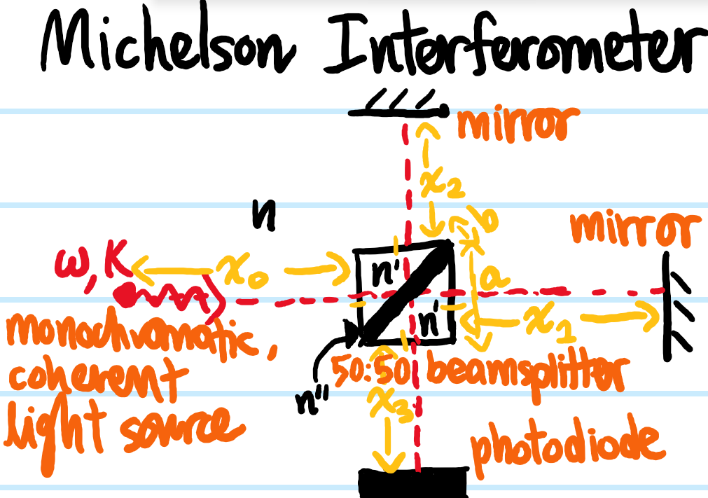
For now, consider for simplicity a monochromatic light source of frequency \(\omega=ck=nvk=n’v’k=n^{\prime\prime}v^{\prime\prime}k\). In “chronological order”, the phases accrued by \(2\) amplitude-split reflected and transmitted rays in their respective journeys from the light source to the photodiode are explicitly:
\[\phi_1=nkx_0+\frac{n’ka}{2}+\pi+\frac{n’ka}{2}+nkx_2+\pi+nkx_2+\frac{n’ka}{2}+\frac{n^{\prime\prime}kb}{\sqrt{1-n’^2/2{n^{\prime\prime}}^2}}+\frac{n’ka}{2}+nkx_3\]
\[\phi_2=nkx_0+\frac{n’ka}{2}+\frac{n^{\prime\prime}kb}{\sqrt{1-n’^2/2{n^{\prime\prime}}^2}}+\frac{n’ka}{2}+nkx_1+\pi+nkx_1+\frac{n’ka}{2}+\pi+\frac{n’ka}{2}+nkx_3\]
where it has been assumed that \(n'<n^{\prime\prime}\) and that \(n<n_{\text{mirrors}}\), though as far as their relative phase difference \(\Delta\phi\) is concerned, because \(\textbf R\) is an additive abelian group it will always just be:
\[\Delta\phi=|\phi_2-\phi_1|=2nk\Delta x\]
where the arm-length difference is \(\Delta x:=|x_2-x_1|\) (to get a \(50:50\) beam splitter there should also be some constraint on \(a,b,n,n’,n^{\prime\prime}\) coming from the Fresnel equations). If the photodiode has sampling period \(T_s>0\), then one expects that the signal it measures will be a time-averaged irradiance of the form (it is being assumed here that the beam splitter really is exactly \(50:50\)):
\[I\sim\langle|e^{-i\omega t}+e^{i\Delta\phi}e^{-i\omega t}|^2\rangle_{T_s}\sim 1+\cos\Delta\phi\sim\cos^2nk\Delta x\]
where \(\cos\Delta\phi\) is the interference term which is sensitive to the relative phase difference \(\Delta\phi\) between the two interfering waves of identical frequency \(\omega\).
On the other hand then, given two distinct frequencies \(\omega<\omega’\) separated by \(\Delta\omega:=\omega’-\omega>0\), one can repeat the story above, this time measuring an irradiance:
\[I\sim\langle|(1+e^{i\Delta\phi})e^{-i\omega t}+(1+e^{i\Delta\phi’})e^{-i\omega’ t}|^2\rangle_{T_s}\sim 1+\cos\frac{\Delta\phi+\Delta\phi’}{2}\cos\frac{\Delta\phi’-\Delta\phi}{2}\]
where the coupled interference cross-term:
\[\frac{\sin\Delta\omega T_s+\sin(\Delta\omega T_s-\Delta\phi’)+\sin(\Delta\omega T_s+\Delta\phi)+\sin(\Delta\omega T_s+\Delta\phi-\Delta\phi’)}{\Delta\omega T_s}\]
is only non-negligible in the limit \(\Delta\omega T_s\ll 1\) which is typically not satisfied, and so here is taken to vanish. The key takeaway from this is that, while any two waves will interfere, waves of distinct frequencies \(\omega’\neq\omega\) do not in general interfere in an easy-to-measure way, i.e. only interference between waves of the same frequency \(\omega\) tends to be measurable.
That being said, it is essential to stress that interference between waves of the same \(\omega\) is interference nonetheless, and the resultant interference pattern \(I(\Delta\phi,\Delta\phi’)\) is readily measured in experiments and still extremely useful. One example of this is in the case where \(\Delta\omega\) is small, such as between \(2\) atomic fine or hyperfine transitions. Then the interference pattern can be written as a function of the Michelson interferometer arm-length difference \(\Delta x\):
\[I(\Delta x)\sim 1+\cos n(k+k’)\Delta x\cos n(k’-k)\Delta x\]
This is analogous to the phenomenon of beats in the \(t\)-domain; here in a spatial domain \(\Delta x\), the low-frequency envelope \(\cos n(k’-k)\Delta x\) is modulated by high-frequency fringes \(\cos n(k+k’)\Delta x\). By finding a \(\Delta x=\Delta x_0\) where fringes disappear due to vanishing of the envelope \(\Delta k:=k’-k=\pi/2n\Delta x_0\), one can thereby obtain the frequency difference \(\Delta\omega=nv\Delta k\) assuming \(n\) is non-dispersive. The envelope is sometimes phrased in terms of the fringe visibility:
\[V(\Delta x):=\frac{\Delta I_{\text{envelope}}(\Delta x)}{\bar I(\Delta x)}=\cos n(k’-k)\Delta x\]
As its name suggests, when the fringes become invisible (i.e. fringe visibility becomes \(V(\Delta x_0)=0\)), then one again recovers the same frequency difference \(\Delta\omega\) as above.
Another point implicitly assumed above and worth stressing is that the relative phase difference \(\Delta\phi\) of the two interfering waves have to maintain temporal coherence \(\frac{\partial\Delta\phi}{dt}=0\) at the photodiode position.
More generally, assuming that waves of any two distinct frequencies, no matter how close, do not interfere, a highly polychromatic signal containing irradiance \(2\hat I(k)dk\) in the wavenumber interval \([k,k+dk]\) would be expected to exhibit a Michelson interference pattern of the form:
\[I(\Delta x)=2\int_0^{\infty}\hat I(k)(1+\cos nk\Delta x)dk\]
Or equivalently, because \(\hat I(\Delta x)\in\textbf R\) is expected to be real-valued for all \(\Delta x\), it follows that its Fourier transform \(\hat I(k)\) needs to be Hermitian \(\hat I(-k)=\hat I^{\dagger}(k)\). This means one can rewrite this as an inverse Fourier transform:
\[I(\Delta x)=I_0+\int_{-\infty}^{\infty}\hat I(k)e^{ink\Delta x}dk\]
with \(I_0=\int_{-\infty}^{\infty}\hat I(k)dk\) the background irradiance. The Fourier transform then provides the spectrum of the light source:
\[\hat I(k)=\int_{-\infty}^{\infty}(I(\Delta x)-I_0)e^{-ink\Delta x}dx\]
and is the basis of the Fourier transform infrared spectrometer (FTIR) where a Michelson interferometer is employed along with one mirror on a motorized translation stage to vary \(\Delta x\) and a photodiode to measure the corresponding total interference pattern \(I(\Delta x)\) from all the wavenumbers \(k\in(0,\infty)\).
Note in all of the above discussion it has been implicitly assumed that all the beams in the Michelson interferometer are perfectly collimated, etc. so that the photodiode observes an interference pattern \(I(\Delta x)\) which would vary with arm-length difference \(\Delta x\) but spatially across the photodiode surface would be uniform; in practice, due to misalignment (accidental or deliberate) or imperfect collimation because the light source is not a point but extended, etc. there is not only an interference pattern in \(\Delta x\)-space, but in real space \((x,y)\) across the photodiode surface too; this whole interference profile \(I(x,y,\Delta x)\) would then change as \(\Delta x\) were to evolve (this is best understood by putting one’s eye at the photodiode location and looking into the beam splitter; one would then see \(2\) virtual images of the light source behind a mirror sitting around \(\sim 2 x_2\) away, separated by \(\sim 2\Delta x\). Conceptually, one can then just forget about the whole Michelson interferometer setup and pretend as if one just had \(2\) coherent light sources interfering with each other on a distant screen. Using this perspective, it is clear that the spatial fringes one observes will be sections of hyperbolae.
Finally, it is worth mentioning that sometimes a minor variant of the Michelson interferometer (called a Twyman-Green interferometer) is used for better collimation of the incident light beam. In addition, if instead of a beam splitter one were to use a half-silvered mirror, then a compensator may also need to be added (this would compensate not only for the optical path length difference in monochromatic incident light but also for optical dispersion in the case of polychromatic incident light).
Mach-Zehnder Interferometer
The setup is the following:
- Kinda similar to Michelson except light never retravels its path.
- Also, instead of a single photodiode on which equal-frequency waves interfere, have two photodiodes to measure the intensities on each output port of the last beamsplitter.
- Idea is that for a \(50:50\) beamsplitter, a unitary (probability-conserving) to describe action on photon probability amplitudes for going down each arm of the Mach-Zehnder.
Fabry-Perot Interferometer
Miscellaneous: Thin Film Interferometer, Haidinger Fringes & Newton’s Rings
Problem: Write down the conditions for maximum constructive and destructive interference in a thin-film interferometer.
Solution: For a light wave incident at angle \(\theta\):
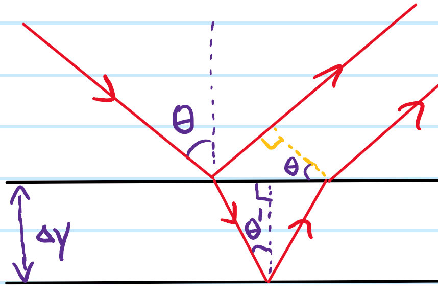
This is the phase shift between the amplitude-split waves arising solely from their path length difference and the magnitude of the impedance mismatch between the \(2\) dielectrics. However, depending on the sign of this impedance mismatch (i.e. whether \(k>k’\) or \(k<k’\)), one of the waves will, at one of the reflections, also accrue an additional \(\pi\) phase shift. So the total phase shift is actually:
\[\Delta\phi=2k_y’\Delta y+\pi\]
and from this the condition for maximum constructive interference \(\Delta\phi=2\pi m\) or maximum destructive interference \(\Delta\phi=2\pi m+\pi\) can be written. To actually compute the resultant light wave’s electric and magnetic fields, one would have to use the Fresnel equations, separately looking at \(s\) and \(p\)-polarized light.
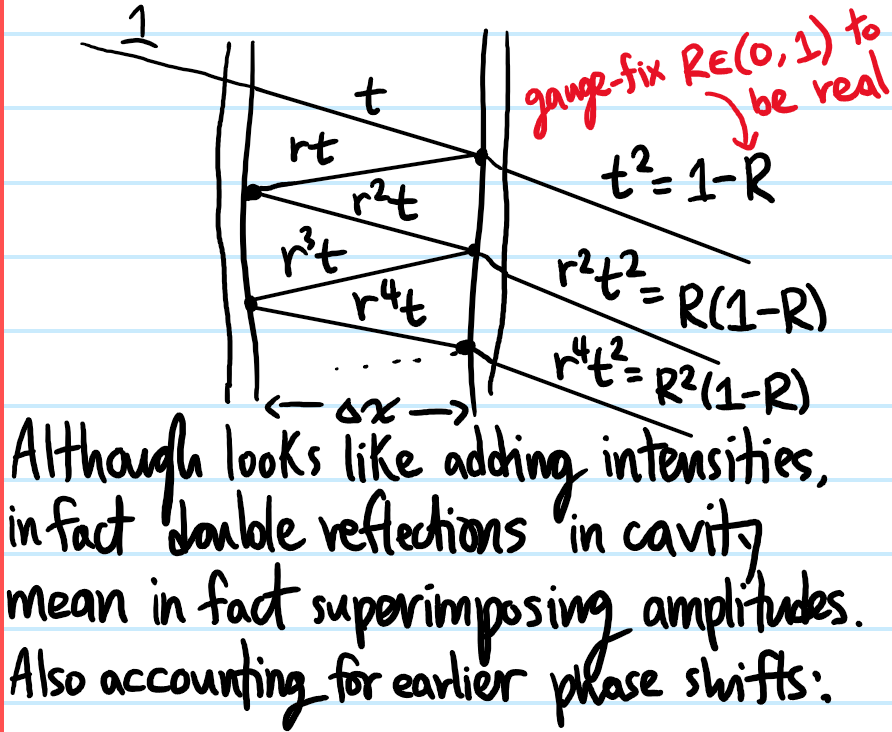
Problem: Show geometrically that the same result applies in a Fabry-Perot interferometer, except the only difference now is that the amplitude is split at transmission/reflection from a low-\(Z\) to high-\(Z\) dielectric, contributing an additional \(\pi\) phase shift not present in the thin-film interferometer, so in total it’s \(2\pi\equiv 0\).
Solution:
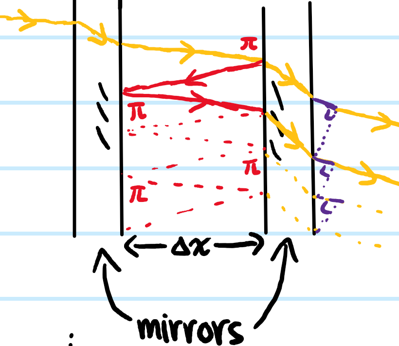
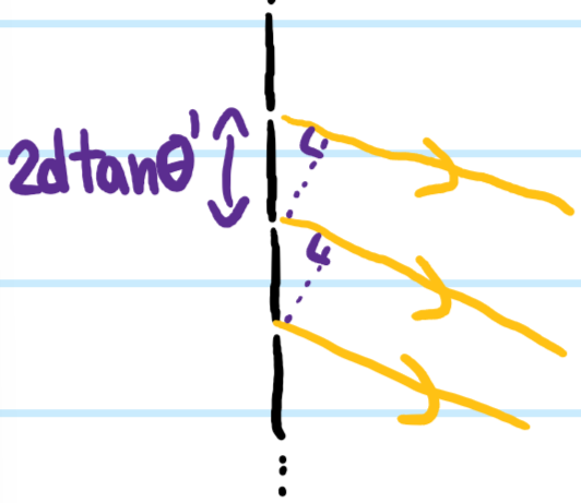
One can also view the Fabry-Perot interferometer as a black box in which case it just behaves like a diffraction grating with slit spacing \(2\Delta x\tan\theta’\), though one also has to account for the extra optical path length traversed inside the optical cavity which can be modelled by an effective glass wedge that phase shifts each beam by a constant \(2k’\Delta x/\cos\theta’\) with respect to its nearest neighbours):
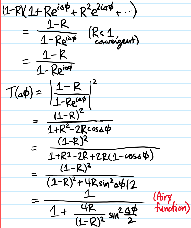
Problem: Now one would like to do better, improving on the previous result. Specifically, one would not only like to know when maxima occur, but also the shape of the FPI’s transmission function \(T(\Delta\phi)\) (i.e. the fraction of the incident power transmitted as a function of the phase shift \(\Delta\phi\) between nearest neighbour reflections). To this end, show that such a transmission function is given by the Airy formula:
\[T(\Delta\phi)=\frac{1}{1+\frac{4R}{(1-R)^2}\sin^2(\Delta\phi/2)}\]
where \(R\) is the reflectivity of either mirror (assumed to be identical), and \(\Delta\phi=2k_x’\Delta x\).

Solution:
Problem: Verify using the Airy transmission function the earlier claim in Problem … that maximum constructive interference occurs when \(\Delta\phi=2\pi m\).
Solution: The Airy transmission function \(T(\Delta\phi)\) is maximized when its denominator is minimized, which occurs when the positive semi-definite part is \(0\), i.e. \(\sin\Delta\phi/2=0\Rightarrow\Delta\phi/2=m\pi\Rightarrow\Delta\phi= 2\pi m\).
Problem: From the plot, it is clear that as one polishes the mirrors more, increasing their reflectivity \(R\), the transmission resonances of the Fabry-Perot occurring (as verified in the previous part) at \(\Delta\phi=2\pi m\) are getting sharper and sharper. Quantify this phenomenon by writing down a formula for the width of the peak.
Solution: The peak clearly has a Lorentzian feel to it, and indeed this can be made explicit by Taylor expanding the \(\sin\) function, choosing the \(m=0\) resonance for simplicity (periodicity ensures they are all identical):

Problem: In analogy to the quality factor \(Q\) of a damped harmonic oscillator, define the finesse \(\mathcal F\) of the Fabry-Perot interferometer (it similarly measures the “quality” of the FPI).
Solution: Just as \(Q=\omega_0/\Delta\omega\), one can analogously define:
\[\mathcal F=\frac{2\pi}{\Delta\phi_{\text{FWHM}}}=\frac{\pi\sqrt{R}}{1-R}\]
where the \(2\pi\) can be interpreted in analogy to \(\omega_0\) as being where the first transmission resonance lies (apart from the one at \(\Delta\phi=0\)), though of course this is actually the separation between any pair of nearest neighbour transmission resonances (which one can loosely refer to as the free spectral range \(\Delta\phi_{\text{FSR}}=2\pi\)).
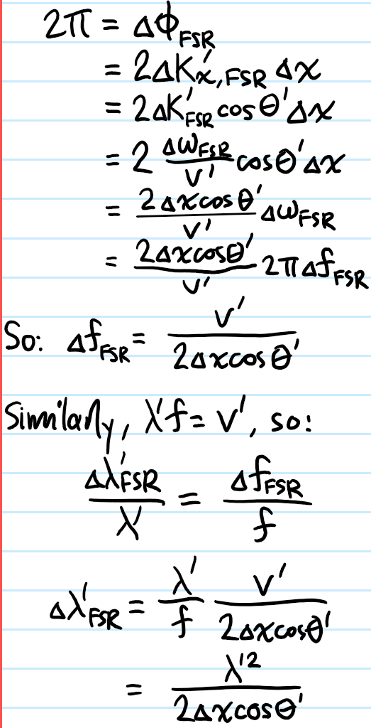
Problem: It is customary to speak of the free spectral range not in \(\Delta\phi\)-space, but when the FPI’s transmission comb is plotted in \(f\)-space or \(\lambda’\)-space. Using \(\Delta\phi_{\text{FSR}}=2\pi\) as the starting point, find expressions for \(\Delta f_{\text{FSR}}\) and \(\Delta\lambda_{\text{FSR}}\) (strictly speaking, a bunch of places where \(\Delta\phi\) is written should really be written as \(\Delta\Delta\phi\) and read as “the difference in delta-phis”)
Solution:
Problem: Although the finesse \(\mathcal F\) was defined in analogy to a \(Q\)-factor in \(\Delta\phi\)-space, show that it also behaves more intimately like a genuine \(Q\)-factor in \(\omega\)-space (and hence also \(f\)-space)!
Solution:
\[\frac{\Delta f_{\text{FSR}}}{\Delta f_{\text{FWHM}}}=\frac{\Delta\phi_{\text{FSR}}}{\Delta\phi_{\text{FWHM}}}=\mathcal F\]
which follows because \(\Delta\phi\) and \(f\) are related by a linear transformation:
\[\Delta\phi=\frac{4\pi\Delta x\cos\theta’}{v’}\Delta f\]
Problem: The line width \(\Delta\lambda’_{\text{FWHM}}\) is often taken to define a “resolution element” of the FPI in \(\lambda’\)-space. This is because, if the incident light is not monochromatic, but say contains \(2\) closely spaced wavelengths \(\lambda’_1,\lambda’_2\), then the FPI will be able to resolve them at the \(m^{\text{th}}\) order iff:
\[\frac{\Delta\lambda}{\lambda’}\geq \frac{1}{m\mathcal F}\]
Show this.
Solution: Starting from the identity:
\[\frac{\Delta\lambda’_{\text{FWHM}}}{\lambda’}=\frac{\Delta f_{\text{FWHM}}}{f}=\frac{\Delta f_{\text{FSR}}}{f\mathcal F}\]
Now write \(f=f_m\) for the frequency of the \(m^{\text{th}}\) order of the FPI in \(f\)-space. Clearly this is just \(f_m=m\Delta f_{\text{FSR}}\) a sequence of \(m\) hops of the free spectral range \(\Delta f_{\text{FSR}}\). This yields the desired result.