
Problem #\(1\): Write down a general \(\phi\)-dependent perturbation to the Klein-Gordon Lagrangian density \(\mathcal L\) for a real scalar field \(\phi\), and explain why in practice only the first \(2\) terms of such a perturbation need to be considered.
Solution #\(1\): Assuming the potential \(V(\phi)\) is analytic in \(\phi\):
\[\mathcal L=\frac{1}{2}\partial^{\mu}\phi\partial_{\mu}\phi-\frac{1}{2}k_c^2\phi^2-\sum_{n\geq 3}\frac{\lambda_n}{n!}\phi^n\]
where the coupling constants \(\lambda_0=\lambda_1=0\), \(\lambda_2=k_c^2\), etc. are not to be confused with the Compton wavelength \(\lambda:=h/mc\). Because the action \(S=\int d^4|X\rangle\mathcal L\) has dimensions of angular momentum \([S]=[\hbar]\) and \([d^4|X\rangle]=[\lambda]^4\), it follows that \([\mathcal L]=[\hbar]/[\lambda]^4=[\hbar^{-3}(mc)^4]\) and thus \([\phi]=[\hbar^{-1/2}mc]\), so:
\[[\lambda_n\phi^n]=[\mathcal L]\Rightarrow [\lambda_n]=[\hbar^{(n-6)/2}(mc)^{4-n}]\]
So on dimensional analysis grounds, the \(n\)-th order coupling constant \(\lambda_n\) does not by itself give a meaningful assessment as to the relevance of the corresponding \(\phi^n\) perturbation, rather it is the dimensionless parameter \(\hbar^{(6-n)/2}(E/c)^{n-4}\lambda_n\) (where \([E]=[mc^2]\) is the relevant energy scale of the process/physics at work) that really matters, i.e. the \(n\)-th order \(\phi^n\) perturbation is small iff \(\hbar^{(6-n)/2}(E/c)^{n-4}\lambda_n\ll 1\).
By graphing \(\hbar^{(6-n)/2}(E/c)^{n-4}\lambda_n\) as a function of \(E\) and given the non-negotiable fact that one is typically interested in “low-\(E\) physics”, it follows that all the \(\phi^n\) couplings for \(n\geq 5\) are irrelevant at these low energy scales, and instead only the marginal \(\phi^4\) quartic coupling and relevant \(\phi^3\) cubic coupling need to be considered. This analysis is quite deep, and goes to show the power of dimensional analysis.
Problem #\(2\): What does it mean for an interacting QFT to be weakly coupled?
Solution #\(2\): It means that one can legitimately treat higher-order interaction terms as small perturbations of a free QFT, i.e. that perturbation theory is accurate (otherwise it would a strongly coupled QFT which is a whole different beast…)
Problem #\(3\): Derive the Dyson series solution to the linear dynamical system \(\dot{\textbf x}(t)=A(t)\textbf x(t)\) and show that it can be expressed as a time-ordered exponential. Show explicitly that it satisfies the ODE.
Solution #\(3\): First, “normalize” away the uninteresting initial condition \(\textbf x(0)\) by writing \(\textbf x(t)=U(t)\textbf x(0)\) so that \(\dot U(t)=A(t)U(t)\) with \(U(0)=1\). Then integrating both sides:
\[U(t)=1+\int_0^tdt’A(t’)U(t’)\]
And recursively substitute ad infinitum:
\[=1+\int_0^tdt’A(t’)\left(1+\int_0^{t’}dt^{\prime\prime}A(t^{\prime\prime})U(t^{\prime\prime})\right)=1+\int_0^tdt’A(t’)+\int_0^tdt’\int_0^{t’}dt^{\prime\prime}A(t’)A(t^{\prime\prime})+…\]
Recall that the definition of the time-ordering superoperator \(\mathcal T\) applied to a string of operators \(A_1(t_1)A_2(t_2)…A_n(t_n)\) is to reorder them so that the earliest time operators also act first (i.e. are on the right). For instance, for a string of \(2\) operators:
\[\mathcal T[A_1(t_1)A_2(t_2)]=A(t_1)A(t_2)\Theta(t_1-t_2)+A(t_2)A(t_1)\Theta(t_2-t_1)\]
or for a string of \(3\) operators, there will be \(3!=6\) terms:
\[\mathcal T[A_1(t_1)A_2(t_2)A_3(t_3)]=A_1(t_1)A_2(t_2)A_3(t_3)\Theta(t_1-t_2)\Theta(t_2-t_3)+A_1(t_1)A_3(t_3)A_2(t_2)\Theta(t_1-t_3)\Theta(t_3-t_2)+…\]
In particular, the Dyson series can be equivalently expressed as the time-ordering superoperator \(\mathcal T\) applied to the strings of operators obtained once one Taylor expands the naive exponential solution:
\[e^{\int_0^tA(t’)dt’}:=1+\int_0^tA(t’)dt’+\frac{1}{2}\int_0^tdt’\int_0^tdt^{\prime\prime}A(t’)A(t^{\prime\prime})+\frac{1}{6}\int_0^tdt’\int_0^tdt^{\prime\prime}\int_0^tdt^{\prime\prime\prime}A(t’)A(t^{\prime\prime})A(t^{\prime\prime\prime})+…\]
Applying \(\mathcal T\) (which is linear):
\[\mathcal T[e^{\int_0^tA(t’)dt’}]=1+\int_0^tA(t’)dt’+\frac{1}{2}\int_0^tdt’\int_0^tdt^{\prime\prime}\biggr(A(t’)A(t^{\prime\prime})\Theta(t’-t^{\prime\prime})+A(t^{\prime\prime})A(t’)\Theta(t^{\prime\prime}-t’)\biggr)+…\]
\[=1+\int_0^tA(t’)dt’+\frac{1}{2}\int_0^tdt’\int_0^{t’}dt^{\prime\prime}A(t’)A(t^{\prime\prime})+\frac{1}{2}\int_0^tdt’\int_{t’}^{t}dt^{\prime\prime}A(t’)A(t^{\prime\prime})+…\]
Among the \(2\) quadratic terms, the first one looks like the one in the Dyson series, but how about the second one? In fact it is equal to the first term; to see this draw a picture to facilitate interchanging the order of integration:

so it becomes clear that \(\int_0^t dt’\int_{t’}^{t}dt^{\prime\prime}=\int_0^tdt^{\prime\prime}\int_0^{t^{\prime\prime}}dt’\). Finally, if one wishes one can interchange the dummy variables \(t’\leftrightarrow t^{\prime\prime}\) to make the two double integrals look utterly identical. As one may anticipate, it turns out that all \(3!=6\) triple integrals at cubic order also coincide, precisely cancelling the \(1/3!=1/6\) prefactor in the Taylor expansion, etc. so that the Dyson series can indeed be written as a time-ordered exponential.
It is also satisfying to explicitly check that the Dyson series for \(U(t)\) satisfies the ODE:
\[\dot U(t)=\frac{d}{dt}\biggr(1+\int_0^tdt’A(t’)+\int_0^tdt’\int_0^{t’}dt^{\prime\prime}A(t’)A(t^{\prime\prime})+…\biggr)=A(t)+A(t)\int_0^t dt’A(t’)+…=A(t)U(t)\]
Or perhaps a more “slick” derivation is to appeal to the time-ordered exponential form of the Dyson series:
\[\dot U(t)=\frac{d}{dt}\mathcal T[e^{\int_0^tA(t’)dt’}]=\mathcal T\left[\frac{d}{dt}e^{\int_0^tA(t’)dt’}\right]\]
and then recognize that within \(\mathcal T\) all operators commute (e.g. for a string of \(2\) operators it is clear that \(\mathcal T[A_1(t_1)A_2(t_2)]=\mathcal T[A_2(t_2)A_1(t_1)]\)) so one can just differentiate naively:
\[=\mathcal T[A(t)e^{\int_0^tA(t’)dt’}]=A(t)\mathcal T[e^{\int_0^tA(t’)dt’}]\]
where the last step follows because \(t\) is the latest time so it can be “factored out” of \(\mathcal T\) to the left.
Problem #\(4\): Write down the Lagrangian density \(\mathcal L\) for scalar Yukawa QFT. What is the condition for this interacting QFT to be weakly coupled? By inspecting \(\mathcal L\), what charges remain conserved despite the interactions? Obtain the scalar Yukawa Hamiltonian density \(\mathcal H\).
Solution #\(4\): Given a real scalar field \(\phi\) and a complex scalar field \(\psi\):
\[\mathcal L=\frac{1}{2}\partial^{\mu}\phi\partial_{\mu}\phi+\partial^{\mu}\bar{\psi}\partial_{\mu}\psi-\frac{1}{2}k_{\phi}^2\phi^2-k_{\psi}^2\bar{\psi}\psi-g\phi\bar{\psi}\psi\]
where the relevant cubic coupling interaction \(g\phi\bar{\psi}\psi\) will be a small perturbation to the free QFT (so that this interacting QFT is weakly coupled) iff the coupling constant \(g=\lambda_3/6\) satisfies (using the results of Solution #\(1\)):
\[\sqrt{\hbar}g\ll k_{\phi},k_{\psi}\]
Just as for the free theory, since one still has the \(U(1)\) global internal symmetry \(\psi\mapsto e^{i\alpha}\psi\) in spite of the cubic coupling term, one continues to have a conserved charge \(Q=N_{\psi}-N_{\bar{\psi}}\).
Performing the relevant Legendre transforms:
\[\partial_0\phi\mapsto\pi_{\phi}=\partial_0\phi\]
\[\partial_0\psi\mapsto\pi_{\psi}=\partial_0\bar{\psi}\]
\[\partial_0\bar{\psi}\mapsto\pi_{\bar{\psi}}=\partial_0\psi\]
One obtains the Hamiltonian density \(\mathcal H=\mathcal H_{\text{free}}+\mathcal H_{\text{int}}\) for scalar Yukawa QFT, where:
\[\mathcal H_{\text{free}}=\frac{\pi^2_{\phi}}{2}+\frac{1}{2}\biggr|\frac{\partial\phi}{\partial\textbf x}\biggr|^2+\pi_{\bar{\psi}}\pi_{\psi}+\frac{\partial\bar{\psi}}{\partial\textbf x}\cdot\frac{\partial\psi}{\partial\textbf x}+\frac{1}{2}k^2_{\phi}\phi^2+k^2_{\psi}\bar{\psi}\psi\]
and:
\[\mathcal H_{\text{int}}=g\phi\bar{\psi}\psi\]
Problem #\(5\): Within scalar Yukawa QFT, explain why the scattering amplitude for the process \(\phi\to\bar{\psi}\psi\) is non-zero, and hence calculate it to order \(g\); what is an assumption implicit in this question?
Solution #\(5\): The implicit assumption is that the initial and final scattering states \(|t=-\infty\rangle,|t=\infty\rangle\in\mathcal F\) are indeed Fock states of the free QFT, i.e. \(H_{\text{free}}=\int d^3\textbf x\mathcal H_{\text{free}}\)-eigenstates, specifically the Lorentz-normalized excitations of the vacuum:
\[|t=-\infty\rangle:=\sqrt{\frac{2}{\hbar}}\frac{\omega_{\textbf k_{\phi}}}{c}a_{\textbf k_{\phi}}^{\dagger}|0\rangle\]
\[|t=\infty\rangle:=\frac{2\omega_{\textbf k_{\bar{\psi}}}\omega_{\textbf k_{\psi}}}{\hbar c^2}b_{\textbf k_{\psi}}^{\dagger}c_{\textbf k_{\bar{\psi}}}^{\dagger}|0\rangle\]
After a long time, in the interaction picture the initial state \(|t=-\infty\rangle\) evolves to \(\mathcal T\exp\left(-\frac{i}{\hbar}\int_{-\infty}^{\infty}dtH_{\text{int}}\right)|t=-\infty\rangle\) (where \(H_{\text{int}}\) is the interaction Hamiltonian in the interaction picture). The overlap of this with a particular final state \(|t=\infty\rangle\) thus yields the probability amplitude of that scattering process:
\[\langle t=\infty|\mathcal T\exp\left(-\frac{i}{\hbar}\int_{-\infty}^{\infty}dtH_{\text{int}}\right)|t=-\infty\rangle\]
where this is expected to be non-zero because \(Q=0\) is conserved in this process. If one is only interested in computing this scattering amplitude to order \(g\), then as usual one Taylor expands the time-ordered exponential to first order:
\[\approx \langle t=\infty|t=-\infty\rangle-\frac{i}{\hbar}\langle t=\infty|\int_{-\infty}^{\infty}dt H_{\text{int}}|t=-\infty\rangle\]
In this case, the initial and final states are orthogonal \(\langle t=\infty|t=-\infty\rangle=0\) which follows intuitively because a \(\phi\)-particle is not the same as a \(\bar{\psi}\psi\)-particle antiparticle pair, or mathematically the creation operators of the different particles all commute so either \(a_{\textbf k_{\phi}}^{\dagger}\) annihilates the bra \(\langle 0|\) or \(b_{\textbf k_{\psi}},c_{\textbf k_{\bar{\psi}}}\) annihilate the ket \(|0\rangle\).
The \(\mathcal O(g)\) matrix element term simplifies to:
\[-\frac{i}{\hbar c}\int d^4|X\rangle\langle t=\infty|\mathcal H_{\text{int}}|t=-\infty\rangle\sim-ig\int d^4|X\rangle\langle 0|b_{\textbf k_{\psi}}c_{\textbf k_{\bar{\psi}}}\phi\bar{\psi}\psi a_{\textbf k_{\phi}}^{\dagger}|0\rangle\]
At this point one has to pull out the Fourier normal mode plane wave expansions of \(\phi,\psi,\bar{\psi}\) (with time dependence since operators evolve in the interaction picture as if they were in the Heisenberg picture of the free QFT), annihilate as much as you can and otherwise use commutation relations to pick up delta functions where needed to do the \(13\)-dimensional integral. When the dust settles, one finds that the scattering amplitude for the process goes like \(-ig\delta^4|K_{\psi}+K_{\bar{\psi}}-K_{\phi}\rangle\) so it’s zero unless \(4\)-momentum is conserved. As a corollary, in the ZMF (rest frame) of the \(\phi\)-particle, one can check that this implies \(m_{\phi}\geq 2m_{\psi}\).
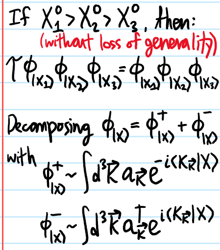
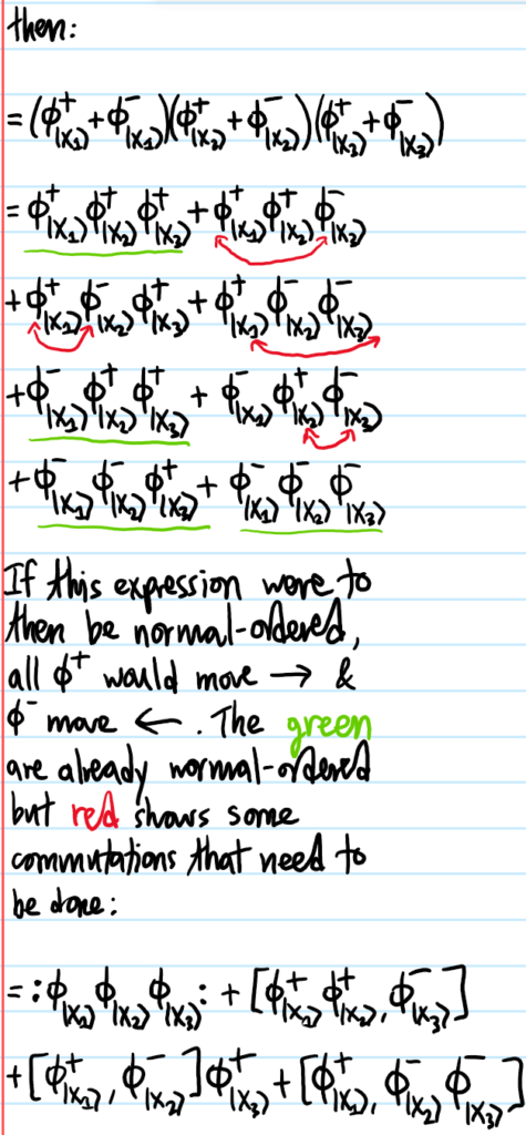
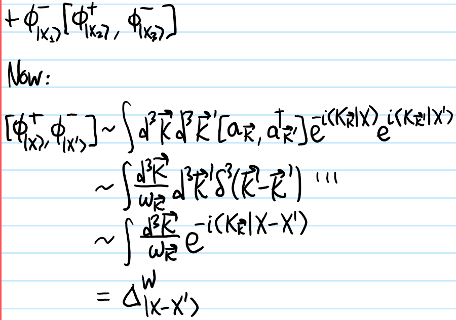
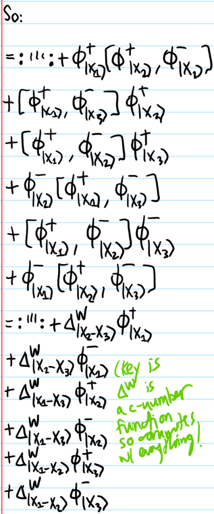
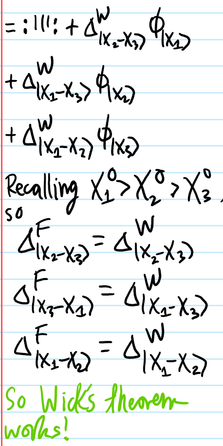
Problem #\(6\): Verify Wick’s theorem for the case of \(3\) scalar fields:
\[\mathcal T\phi_{|X_1\rangle}\phi_{|X_2\rangle}\phi_{|X_3\rangle}=:\phi_{|X_1\rangle}\phi_{|X_2\rangle}\phi_{|X_3\rangle}:+\Delta^F_{|X_2-X_3\rangle}\phi_{|X_1\rangle}+\Delta^F_{|X_3-X_1\rangle}\phi_{|X_2\rangle}+\Delta^F_{|X_1-X_2\rangle}\phi_{|X_3\rangle}\]
Solution #\(6\):
Problem #\(7\): Within weakly coupled scalar Yukawa QFT, compute the scattering amplitude for the process \(\bar{\psi}\psi\to\bar{\psi}\psi\) at order \(\mathcal O(g^2)\).
Solution #\(7\): At order \(\mathcal O(g^2)\), the scattering amplitude for this interaction from the initial state \(|t=-\infty\rangle\sim b_{\textbf k_1}^{\dagger}b_{\textbf k_2}^{\dagger}|0\rangle\) to the final state \(|t=\infty\rangle=\sim b_{\textbf k’_1}^{\dagger}b_{\textbf k’_2}^{\dagger}|0\rangle\) is given by:
\[\langle t=-\infty|S-1|t=\infty\rangle\sim i\mathcal A_{\bar{\psi}\psi\to\bar{\psi}\psi}\delta^4|K_{\psi}+K_{\bar{\psi}}-K_{\phi}\rangle\]
where to order \(\mathcal O(g^2)\), the “amplitude” \(\mathcal A_{\bar{\psi}\psi\to\bar{\psi}\psi}\) is given by the sum of the following two tree-level Feynman diagrams, namely a \(t\)-channel and a \(u\)-channel:


Problem #\(8\): Repeat Problem #\(7\) for the case of scalar Yukawa scattering of mesons \(\phi\phi\to\phi\phi\) at order \(\mathcal O(g^4)\).
Solution #\(8\): Given that the interaction Hamiltonian density for scalar Yukawa theory is cubic \(\mathcal H_{\text{int}}=g\phi\bar{\psi}\psi\), it follows that any Feynman diagram must be a cubic graph with exactly one \(\phi\)-edge, one \(\psi\)-edge, and one \(\bar{\psi}\)-edge at each vertex of the directed graph. By initially drawing the following:
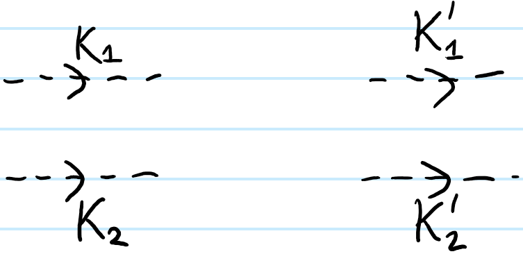
and pondering for a bit, it is intuitively plausible that the simplest way to satisfy the above constraint is for the \(\phi\)-mesons to exchange virtual \(\psi/\bar{\psi}\) nucleons/antinucleons via the following one-loop (no longer tree-level) Feynman diagram:
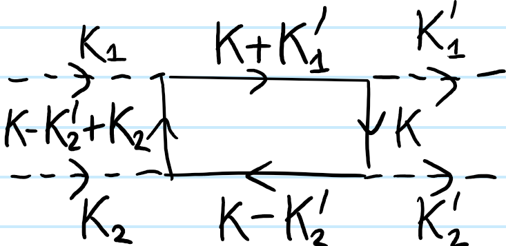
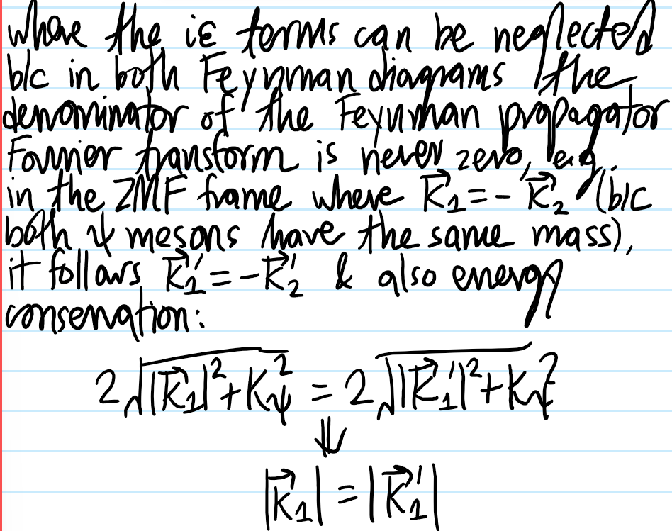
and so because there are \(4\) vertices, it follows that the \(\phi\phi\to\phi\phi\) interaction scattering amplitude is \(\mathcal O(g^4)\). The Feynman rules assert that to \(\mathcal O(g^4)\) it is given by (notation here is a bit loose, in particular \(|\phi\phi\rangle^{\dagger}\neq\langle\phi\phi|\)):
\[\langle\phi\phi|S-1|\phi\phi\rangle\sim i\mathcal A_{\phi\phi\to\phi\phi}\delta^4(K’_1+K’_2-K_1-K_2)\]
where \(\mathcal A_{\phi\phi\to\phi\phi}\) is given by the one-loop integral over \(4\)-momenta:

Problem #\(10\): Define the Mandelstam variables \(s,t,u\in\textbf R\) by drawing suitable \(s\)-channel, \(t\)-channel and \(u\)-channel Feynman diagrams for interactions between two particles (of arbitrary type).
Solution #\(10\):

