Problem: Draw a DNA molecule. Annotate the terms nucleotides, phosphate group, deoxyribose, phosphodiester linkage, adenine, thymine, cytosine, guanine, nitrogenous bases.
Problem: Draw an RNA molecule, and make similar annotations as for DNA.
Problem: What is the typical length scale \(x_{\text{cell}}\) of a cell? How does that compare with the typical width \(x_{\text{hair}}\) of a human hair?
Solution: One has \(x_{\text{cell}}\sim 10\space\mu\text m\), whereas \(x_{\text{hair}}\sim 100\space\mu\text m\), so \(x_{\text{hair}}/x_{\text{cell}}\sim 10\) (though exact values vary!).
Problem: Draw a cartoon cross-section of a typical eukaryotic cell. Annotate the terms nucleus, mitochondria, ribosome, rough endoplasmic reticulum, smooth endoplasmic reticulum, golgi bodies, lysosomes, and (for plants) chloroplasts.
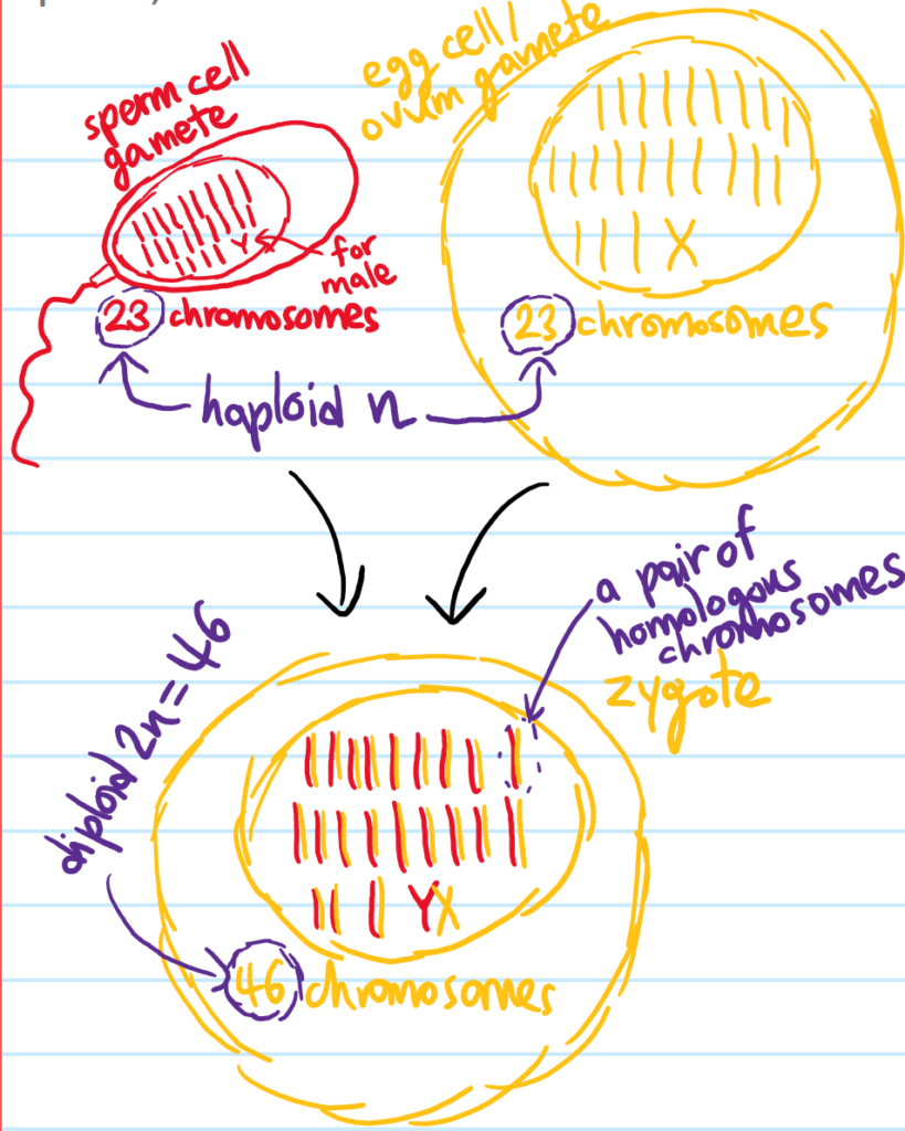
Problem: Draw a diagram depicting the process of fertilization. Annotate the terms gamete, zygote, pair of homologous chromosomes, haploid number, and diploid number on the diagram.
Solution: