
Problem #\(1\): Find the mistake in this derivation of the Green’s function for the inhomogeneous Helmholtz equation subject to the boundary condition of an outgoing wave:
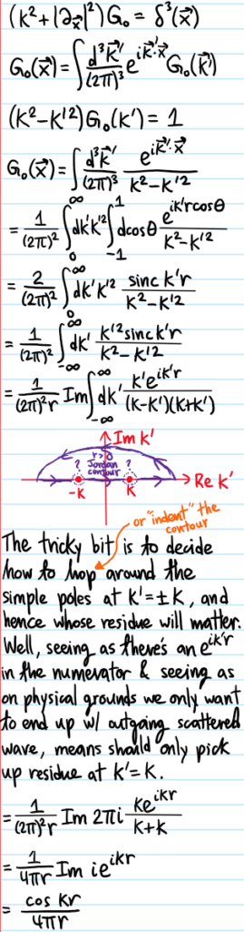
Solution #\(1\): First of all, the correct answer should be \(G(r)=\frac{e^{ikr}}{4\pi r}\), not this standing wave with a \(\cos(kr)=(e^{ikr}+e^{-ikr})/2\) that superposes both an ingoing \(e^{-ikr}\) and outgoing wave \(e^{ikr}\). Reasoning that \(\cos(kr)\in\textbf R\) because it came after hitting with the \(\Im\) function, one might be led (correctly as it turns out) to the conclusion that this step:
\[\int_{-\infty}^{\infty}\frac{k’^2\text{sinc}(k’r)}{k^2-k’^2}\neq\frac{1}{r}\Im\int_{-\infty}^{\infty}dk’\frac{k’e^{ik’r}}{(k-k’)(k+k’)}\]
was the seemingly innocuous but incorrect step. Basically, although it’s certainly true that \(\sin(k’r)=\Im e^{ik’r}\), the difficulty is that in order to be able to pull the \(\Im\) out of the integral, one has to be sure that the prefactor \(\frac{k’^2}{k^2-k’^2}\) is real. But in fact, despite looking very real, it should really have an \(i\varepsilon\) in the denominator (or sometimes just written as \(i0\) to reflect taking the limit \(\varepsilon\to 0\)). It is this slight shifting of the poles at \(k’=\pm k\) off the real axis to \(k’=\pm k\pm’i\varepsilon\) that makes this naive manipulation invalid!
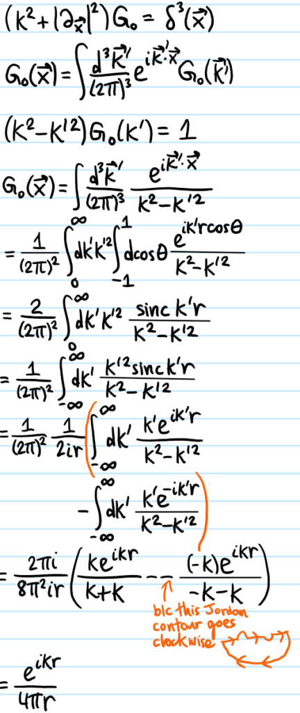
Problem #\(2\): Fix the mistake by redoing the derivation correctly
Solution #\(2\):
Problem #\(3\): Hence write down immediately the Lippman-Schwinger equation in the position representation for scattering off an arbitrary potential \(V\).
Solution #\(3\): All you need to remember is:
\[\left(k^2+\biggr|\frac{\partial}{\partial\textbf x}\biggr|^2\right)\psi=-\frac{2m}{\hbar^2}V\psi\]
where the RHS is viewed as a \(\psi\)-dependent forcing function, so the solution of this inhomogeneous PDE is just the particular integral + complementary function:
\[\psi(\textbf x)=e^{i\textbf k\cdot\textbf x}+\left(G*-\frac{2m}{\hbar^2}V\psi\right)(\textbf x)\]
where the convolution is:
\[\left(G*-\frac{2m}{\hbar^2}V\psi\right)(\textbf x)=-\frac{m}{2\pi\hbar^2}\int d^3\textbf x’V(\textbf x’)\psi(\textbf x’)\frac{e^{ik|\textbf x-\textbf x’|}}{|\textbf x-\textbf x’|}\]
Problem #\(4\): By aligning the incident momentum \(\textbf k=k\hat{\textbf z}\) along the \(z\)-axis and working asymptotically \(|\textbf x-\textbf x’|\approx |\textbf x|-\hat{\textbf x}\cdot\textbf x’\) in the exponent of the Green’s function \(G(r)=e^{ikr}/4\pi r\) while directly approximating \(|\textbf x-\textbf x’|\approx |\textbf x|\), obtain the Fraunhofer-Lippman-Schwinger equation:
\[\psi(\textbf x)=e^{ikz}+f(\hat{\textbf x})\frac{e^{ikr}}{r}\]
where the scattering amplitude \(f(\hat{\textbf x})\) in direction \(\hat{\textbf x}\) is defined by:
\[f(\hat{\textbf x}):=-\frac{m}{2\pi\hbar^2}\int d^3\textbf x’V(\textbf x’)\psi(\textbf x’)e^{-ik\hat{\textbf x}\cdot\textbf x’}\]
Solution #\(4\): Trivial.
Problem #\(5\): What is the scattering amplitude \(f(\hat{\textbf x})\) in the \(1^{\text{st}}\) Born approximation?
Solution #\(5\): Basically, just replace \(\psi(\textbf x’)\mapsto e^{i\textbf k\cdot\textbf x’}\) in the integrand (as that’s the plane wave solution when \(V=0\)). Thus, one finds that, up to some constants, the scattering amplitude \(f(\hat{\textbf x})\) in a given direction \(\hat{\textbf x}\) is determined by the Fourier structure of the potential \(V\), i.e. what is the amplitude of the plane wave in \(V\) travelling in the direction of the momentum transfer \(\textbf k’-\textbf k\):
\[f(\hat{\textbf x})=-\frac{m}{2\pi\hbar^2}\hat V(\textbf k’-\textbf k)\]
where the \(\hat{\textbf x}\)-dependence in \(f(\hat{\textbf x})\) is all inside \(\textbf k’:=k\hat{\textbf x}\).
Problem #\(6\): What about the corresponding cross section \(\sigma\) in the \(1^{\text{st}}\) Born approximation.
Solution #\(6\): \[\sigma=\int d^2\hat{\textbf x}|f(\hat{\textbf x})|^2=\left(\frac{m}{2\pi\hbar^2}\right)^2\int d^2\textbf x’|\hat V(\textbf k’-\textbf k)|^2\]
which is sort of like a Plancherel-type integral.
Problem #\(7\): Apply the \(1^{\text{st}}\) Born approximation to calculate the Rutherford scattering amplitude \(f(\theta)\) in the cone \(\theta\) from a repulsive Coulomb potential.
Solution #\(7\): The Coulomb potential itself is not Fourier transformable, but the Yukawa potential \(V(r)=Ae^{-\kappa r}/r\) (which is like the Helmholtz Green’s function of a bound state?) has \(\hat V(k)=4\pi A/(k^2+\kappa^2)\) (no contour integration is even needed, this integral is very elementary). Then (nonrigorously) taking the limit \(\kappa\to 0\) (i.e. letting the range \(1/\kappa\to\infty\)) reproduces the Coulomb potential with supposed inverse-square Fourier transform \(\hat V(k)=4\pi A/k^2\). So the scattering amplitude in the \(1^{\text{st}}\) Born approximation is thus:
\[f(\hat{\textbf x})=-\frac{2mA}{\hbar^2|\textbf k’-\textbf k|^2}=\frac{A}{4E\sin^2\theta/2}\]
with \(E=\hbar^2k^2/2m\).
Problem: Show that the \(s\)-wave scattering amplitude \(f_s(k)\) is isotropic and related to the \(s\)-wave scattering length \(a_s\) of the isotropic potential \(V(r)\) by the Mobius transformation:
\[f_s(k)\approx-\frac{1}{ik+a^{-1}_s}=-a_s+ika_s^2+O(k^2)\to -a_s\text{ as }k\to 0\]
and hence as \(k\to 0\) the asymptotic wavefunction approaches \(\psi(r)\to 1-\frac{a_s}{r}\).
Solution: The partial wave expansion of the \(z\)-axisymmetric scattering amplitude \(f(\theta)\) in an isotropic potential \(V(r)\) receives contributions from all angular momentum sectors:
\[f(\theta)=\sum_{\ell=0}^{\infty}f_{\ell}(k)P_{\ell}(\cos\theta)\]
with “Legendre coefficients”:
\[f_{\ell}(k)=\frac{2\ell+1}{k}e^{i\delta_{\ell}(k)}\sin\delta_{\ell}(k)\]
For low-energy \(k\to 0\) scattering, the \(\ell=0\) \(s\)-wave contribution dominates so that the scattering amplitude \(f(\theta)\approx f_0(k)P_0(\cos\theta)=f_0(k)=f_s(k)\) is not even a function of \(\theta\) anymore, i.e. it is isotropic!
\[f_s(k)=\frac{e^{i\delta_0(k)}\sin\delta_0(k)}{k}\]
In particular, in the low-energy limit \(k\to 0\) one has \(\delta_0(k)\to 0\) linearly as \(\delta_0(k)=-ka_s+O(k^2)\), so expanding \(\sin\delta_0(k)\approx\delta_o(k)\) and doing the slightly dodgy manipulation of writing \(e^{i\delta_0(k)}=\frac{1}{e^{-i\delta_0(k)}}=\frac{1}{1-i\delta_0(k)}\) one obtains the desired results. The asymptotic wavefunction is:
\[\psi(r,\theta,\phi)=e^{ikz}+f(k,\theta,\phi)\frac{e^{ikr}}{r}\to 1-\frac{a_s}{r}\]
upon setting \(k=0\).