Problem #\(1\): When someone comes up to you on the street and just says “Ising model”, what should be the first thing you think of?
Solution #\(1\): The classical Hamiltonian:
\[H=-E_{\text{int}}\sum_{\langle i,j\rangle}\sigma_i\sigma_j-E_{\text{ext}}\sum_i\sigma_i\]
(keeping in mind though that there many variants on this simple Ising model).
Problem #\(2\): Is the Ising model classical or quantum mechanical?
Solution #\(2\): It is purely classical. Indeed, this is a very common misconception, because many of the words that get tossed around when discussing the Ising model (e.g. “spins” on a lattice, “Hamiltonian”, “(anti)ferromagnetism”, etc.) sound like they are quantum mechanical concepts, and indeed they are but the Ising model by itself is a purely classical mathematical model that a priori need not have any connection to physics (and certainly not to quantum mechanical systems; that being said it’s still useful for intuition to speak about it as if it were a toy model of a ferromagnet).
To hit this point home, remember that the Hamiltonian \(H\) is just a function on phase space in classical mechanics, whereas it is an operator in quantum mechanics…but in the formula for \(H\) in Solution #\(1\), there are no operators on the RHS, the \(\sigma_i\in\{-1,1\}\) are just some numbers which specify the classical microstate \((\sigma_1,\sigma_2,…)\) of the system, so it is much more similar to just a classical (as opposed to quantum) Hamiltonian. And there are no superpositions of states, or non-commuting operators, or any other quantum voodoo going on. So, despite the discreteness/quantization which is built into the Ising model, it is purely classical.
Problem #\(3\): What does it mean to “solve” the Ising model? (i.e. what properties of the Ising lattice is one interested in understanding?)
Solution #\(3\): The mental picture one should have in mind is that of coupling the Ising lattice with a heat bath at some temperature \(T\), and then ask how the order parameter \(m\) of the lattice (in this case the Boltzmann-averaged mean magnetization) varies with the choice of heat bath temperature \(T\). Intuitively, one should already have a qualitative sense of the answer:
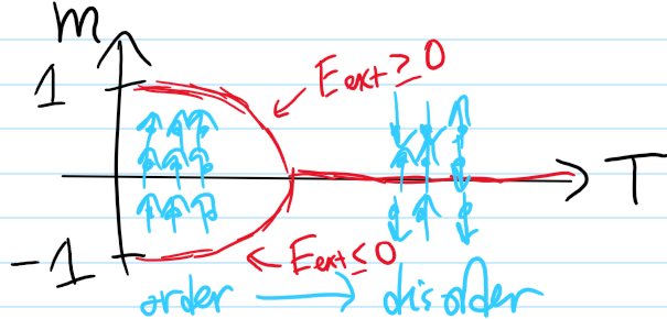
So to “solve” the Ising model just means to quantitatively get the equation of those curves \(m=m(T)\) for all possible combinations of parameters \(E_{\text{int}},E_{\text{ext}}\in\textbf R\) in the Ising Hamiltonian \(H\).
Problem #\(4\):
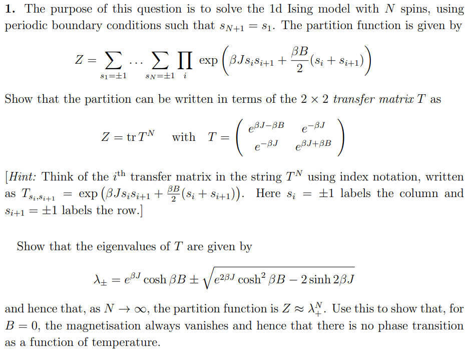
Solution #\(4\):
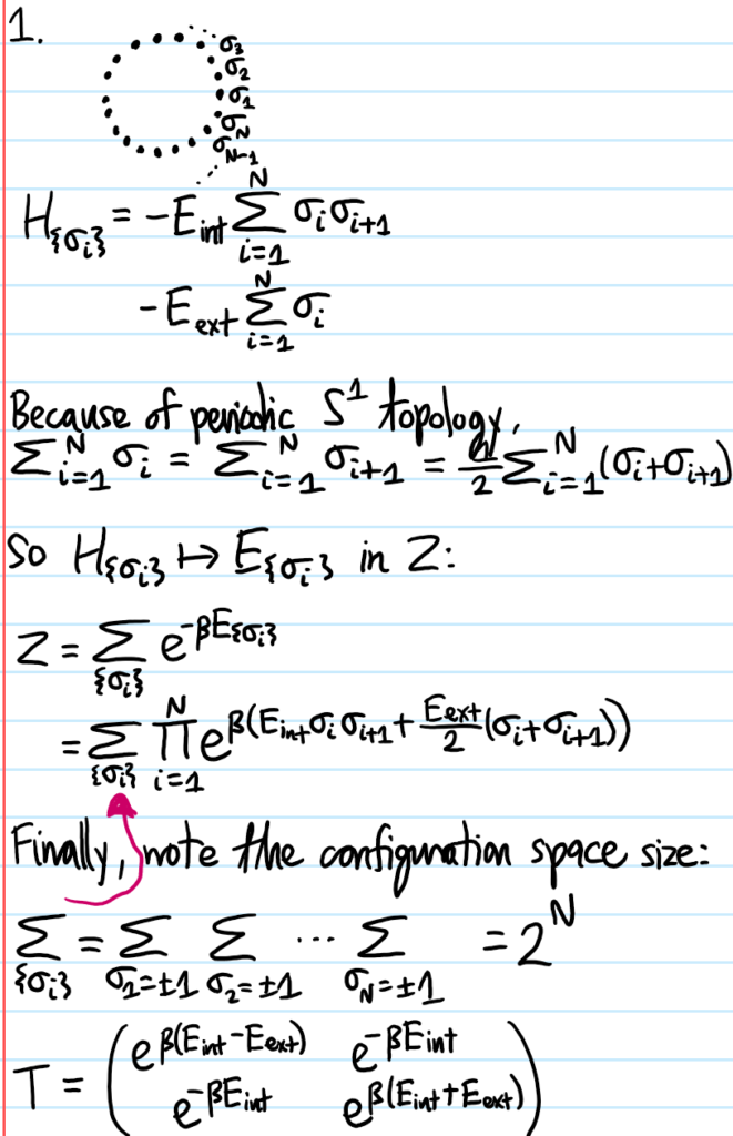
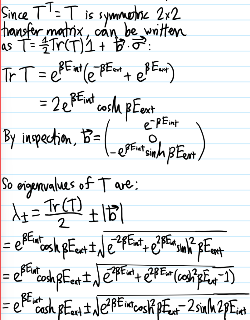
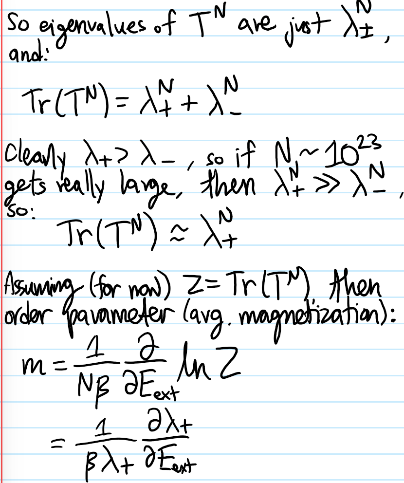
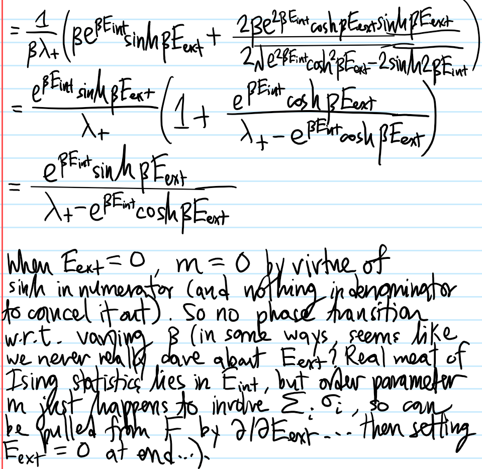
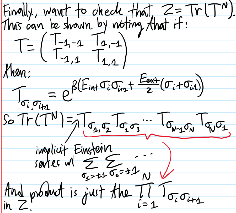
Problem #\(5\):
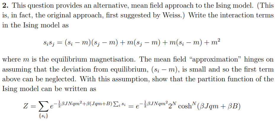

Solution #\(5\):
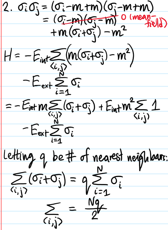
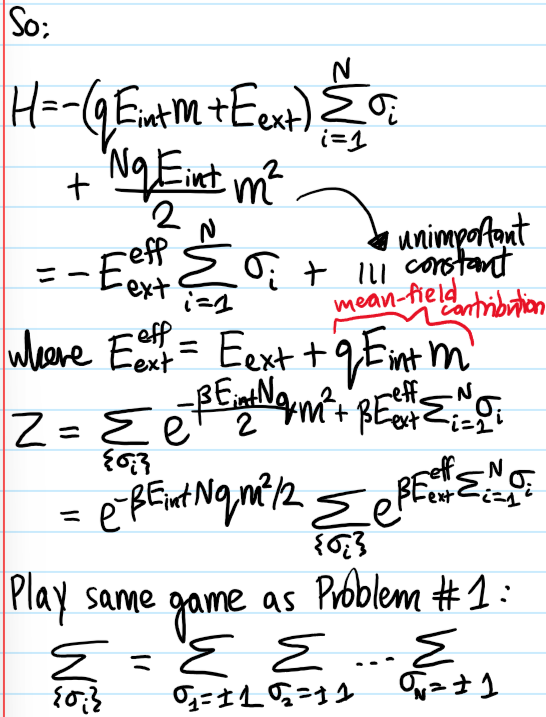
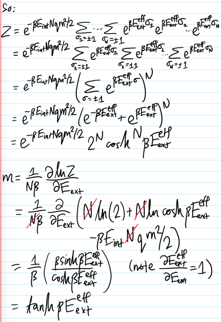
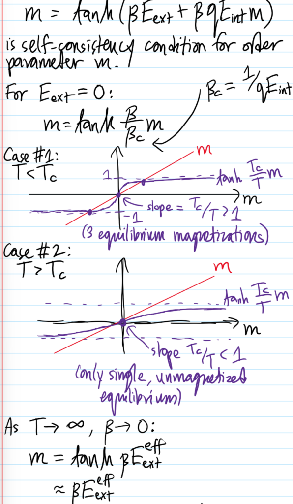
Comparing with the earlier intuitive sketch (note all the inner loop branches at low temperature are unstable):
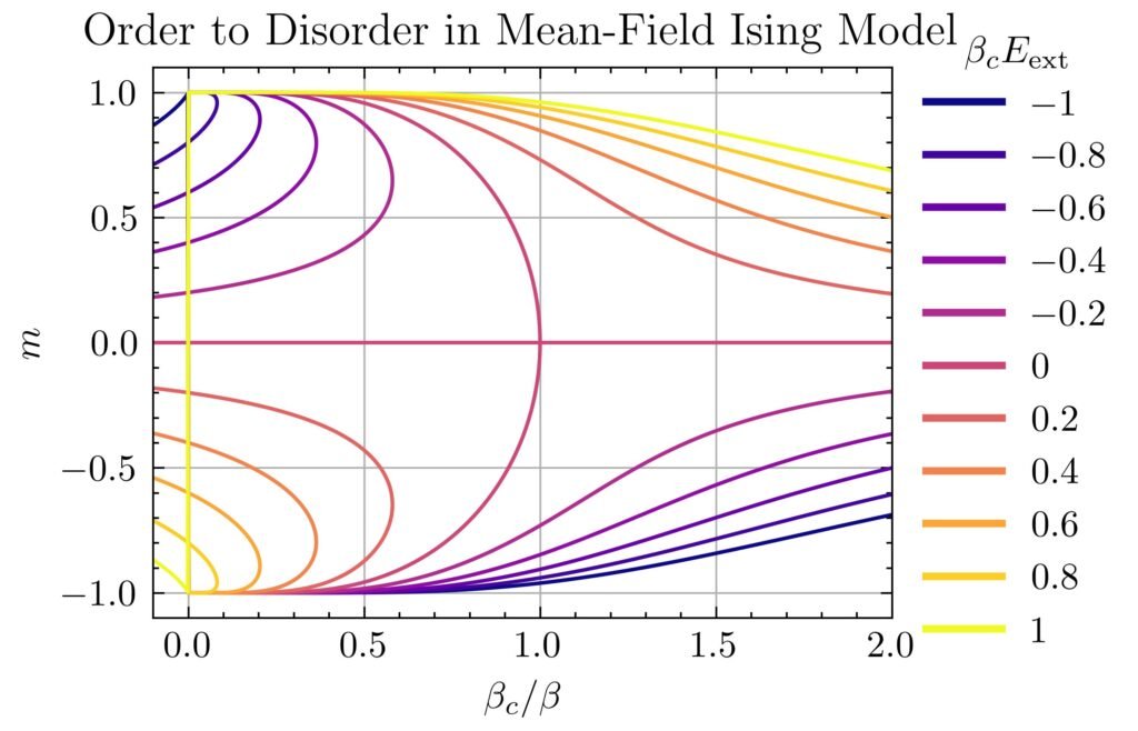
In particular, the phase transition at \(E_{\text{ext}}=0\) is manifest by the trifurcation at the critical point \(\beta=\beta_c\).
Problem #\(6\):
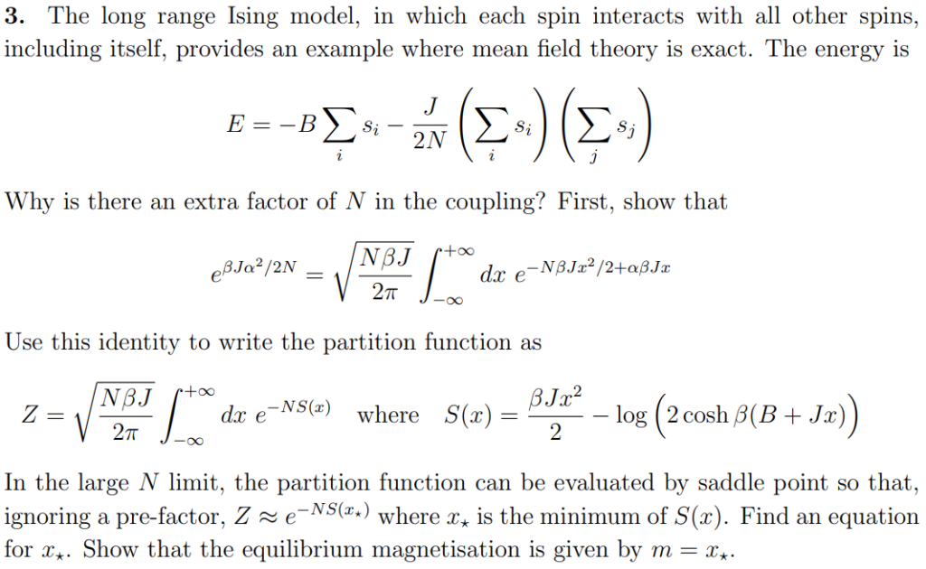
Solution #\(6\):
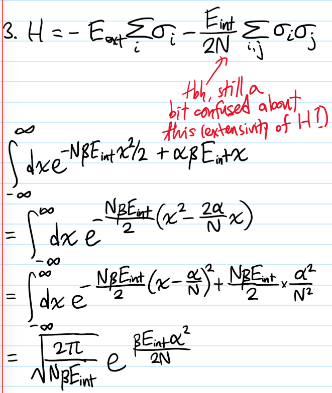
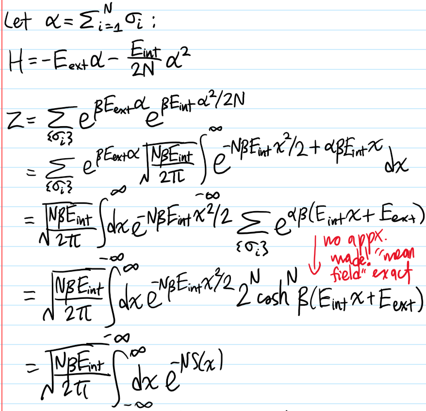
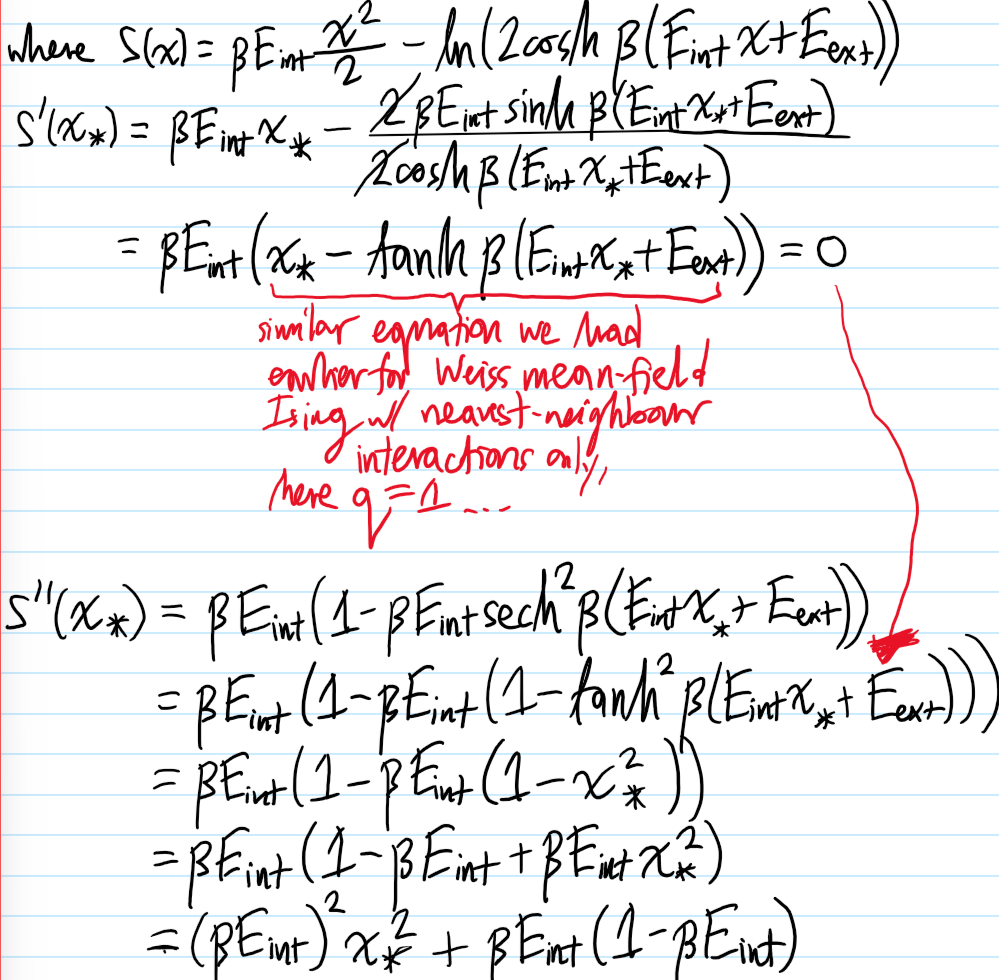
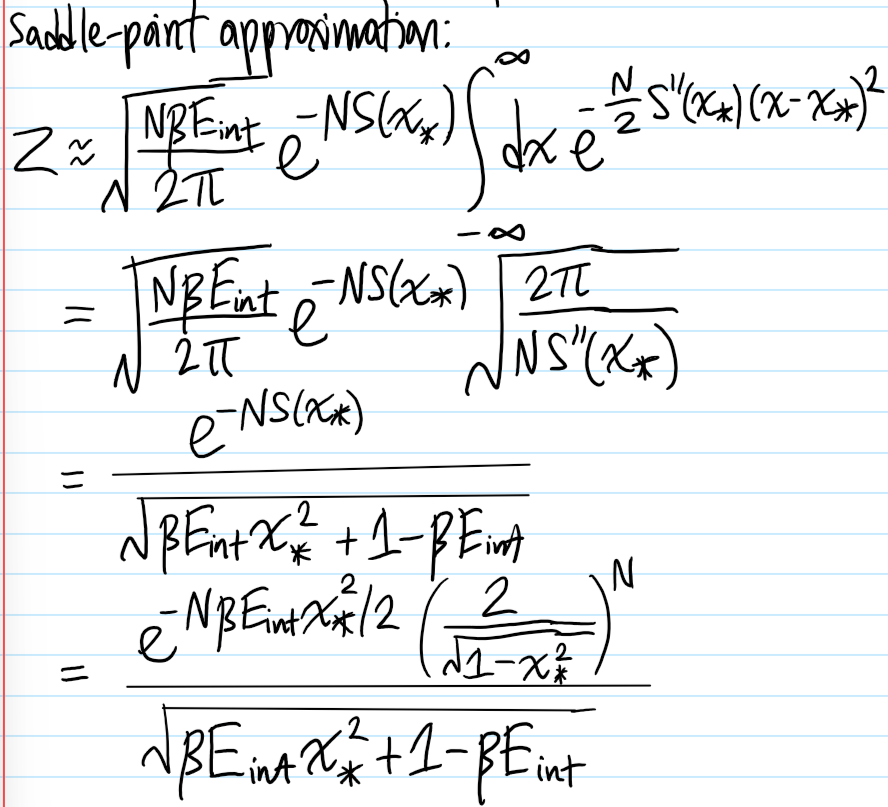
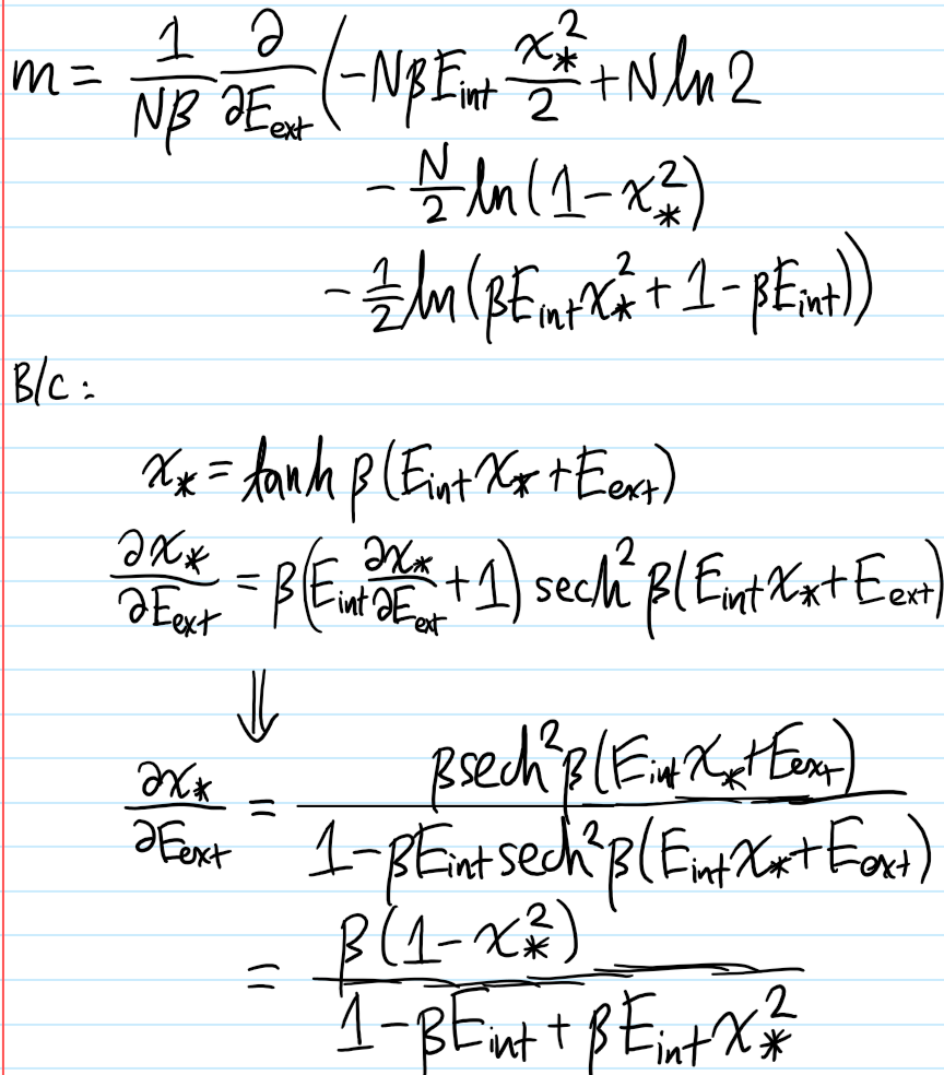
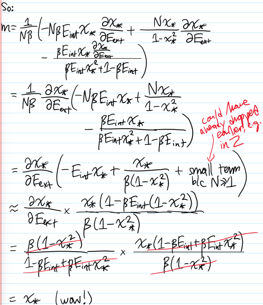
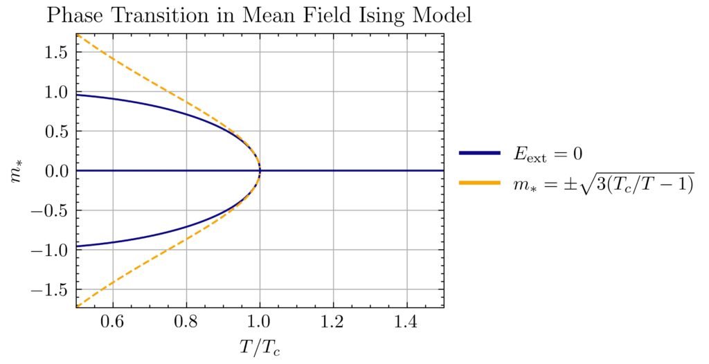
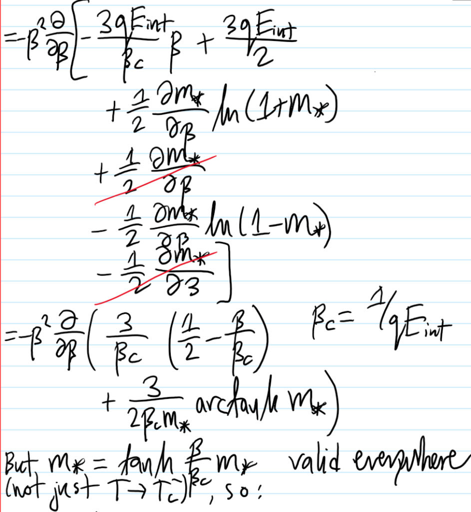
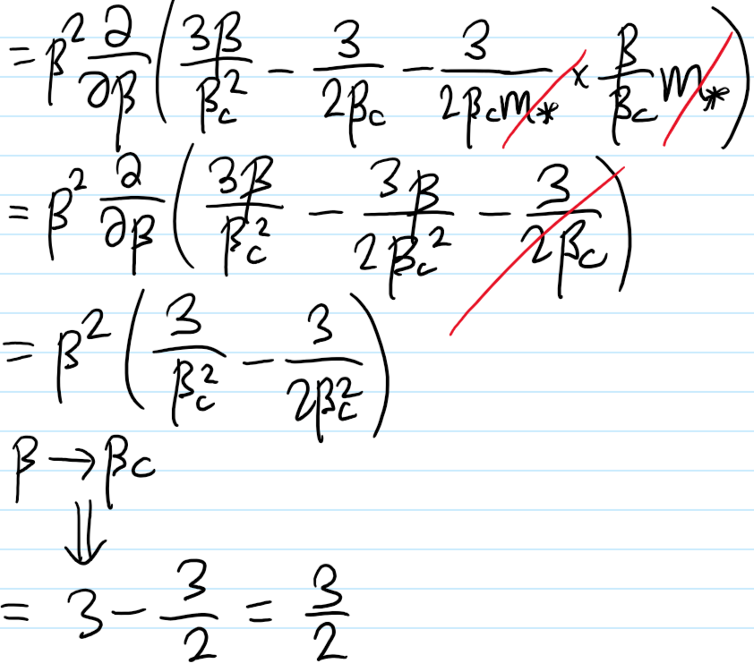
Problem #\(7\): Show that in the mean field approximation, the short-range Ising model at \(E_{\text{ext}}=0\) experiences a \(2\)-nd order phase transition in the equilibrium magnetization \(m_*(T)\) for \(T<T_c\) (but \(T\) close to \(T_c\)) goes like \(m_*(T)\approx\pm\sqrt{3(T_c/T-1)}\).
Solution #\(7\): Within (stupid!) mean-field theory, the effective free energy is:
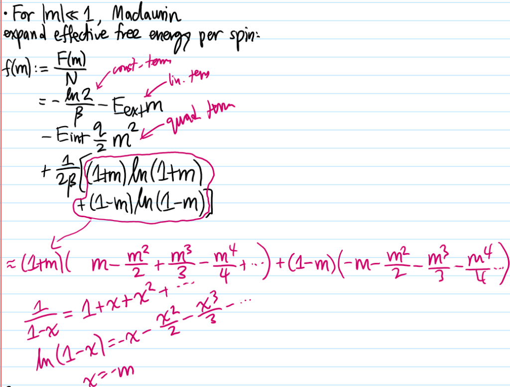
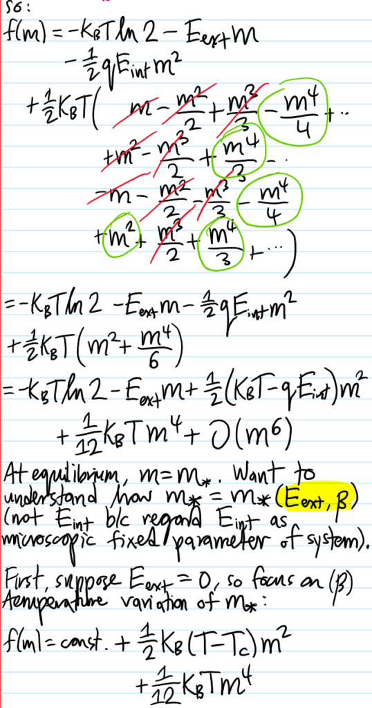
\[f(m)=-k_BT\ln 2-E_{\text{ext}}m-\frac{qE_{\text{int}}}{2}m^2+\frac{1}{2}k_BT\biggr[(1+m)\ln(1+m)+(1-m)\ln(1-m)\biggr]\]
Proof:
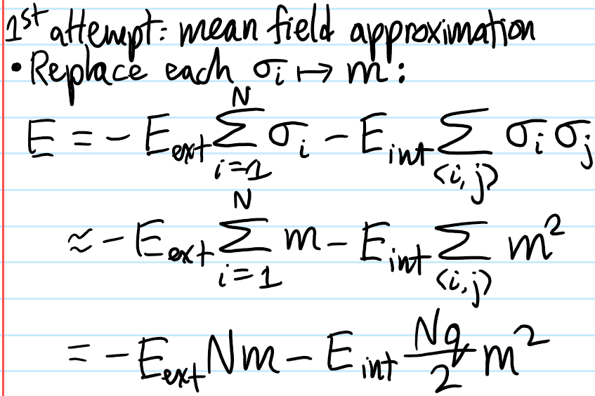
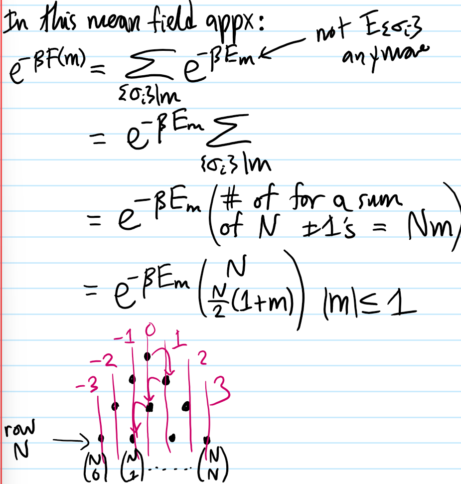
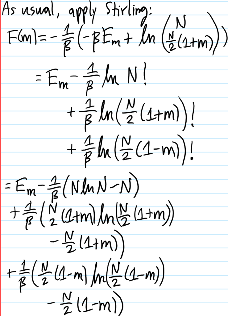
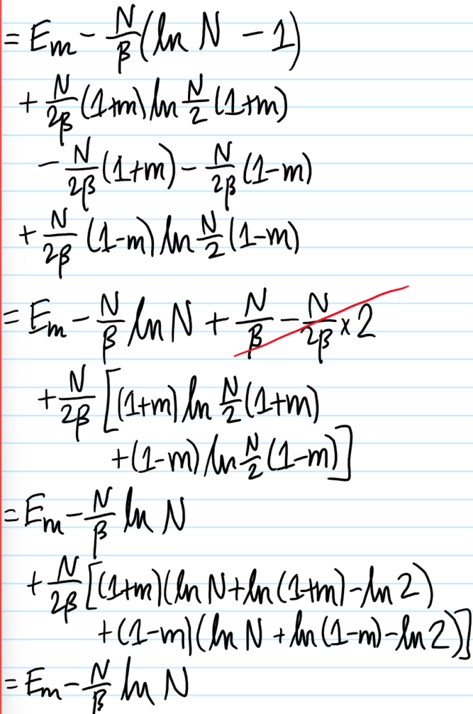
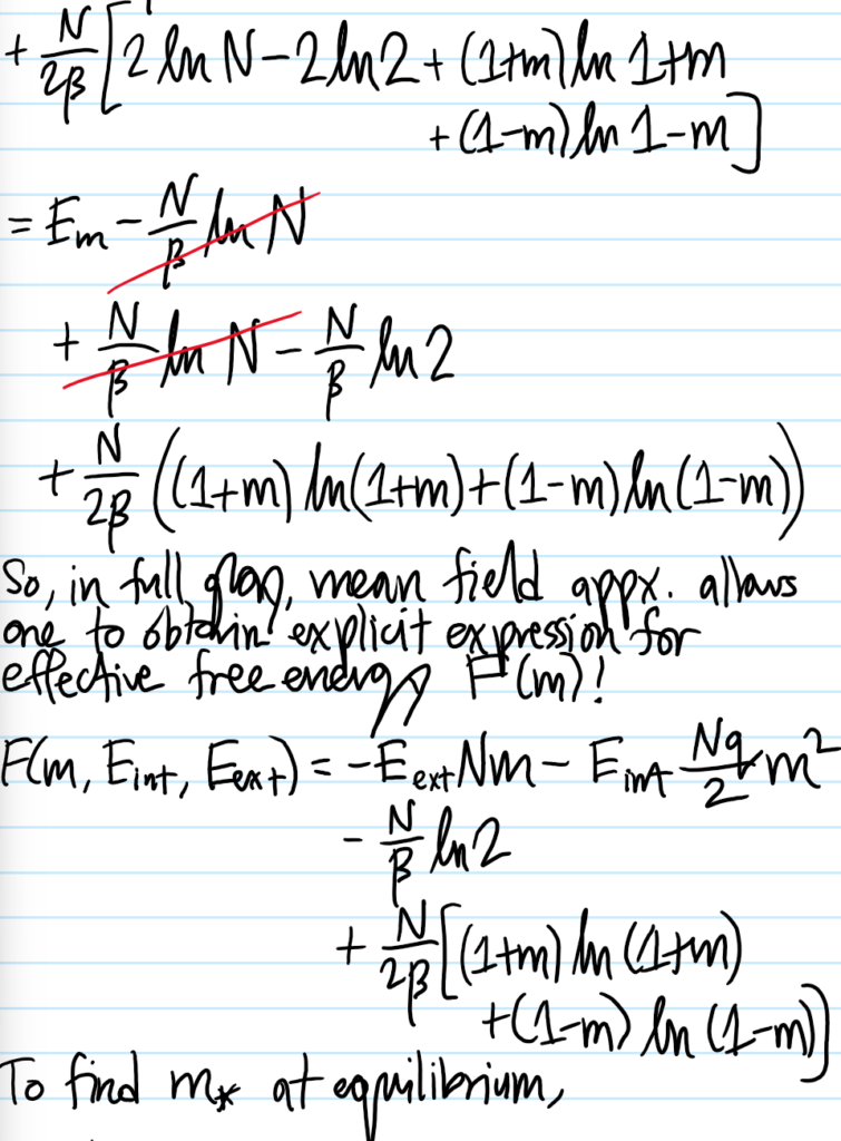
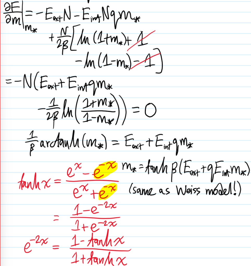
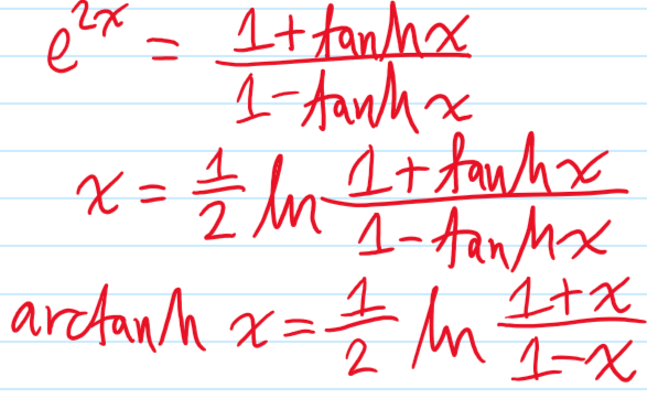
So anyways, Maclaurin-expanding the mean-field effective free energy \(f(m)\) per unit spin:
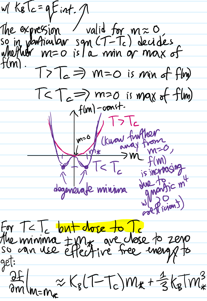
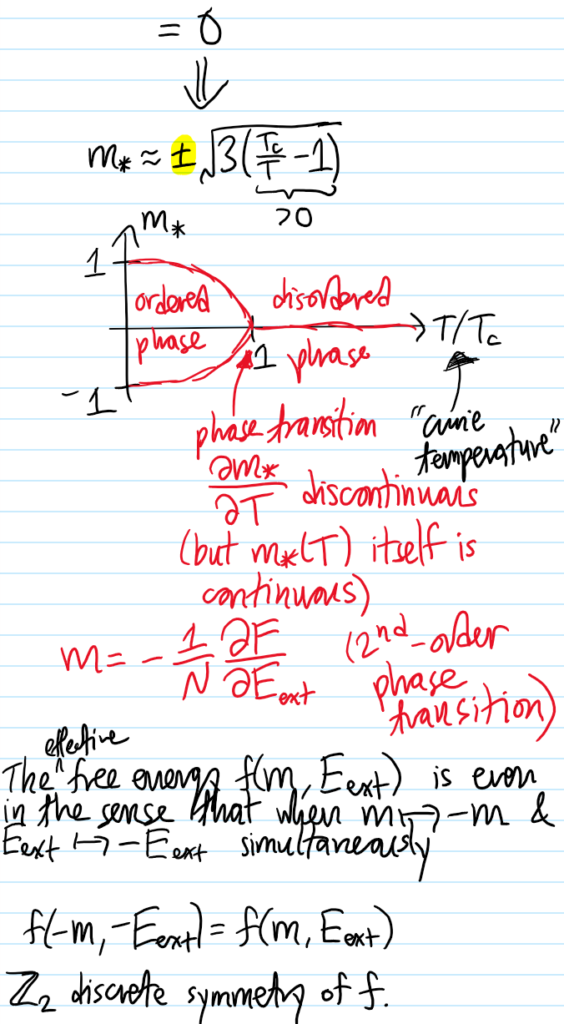
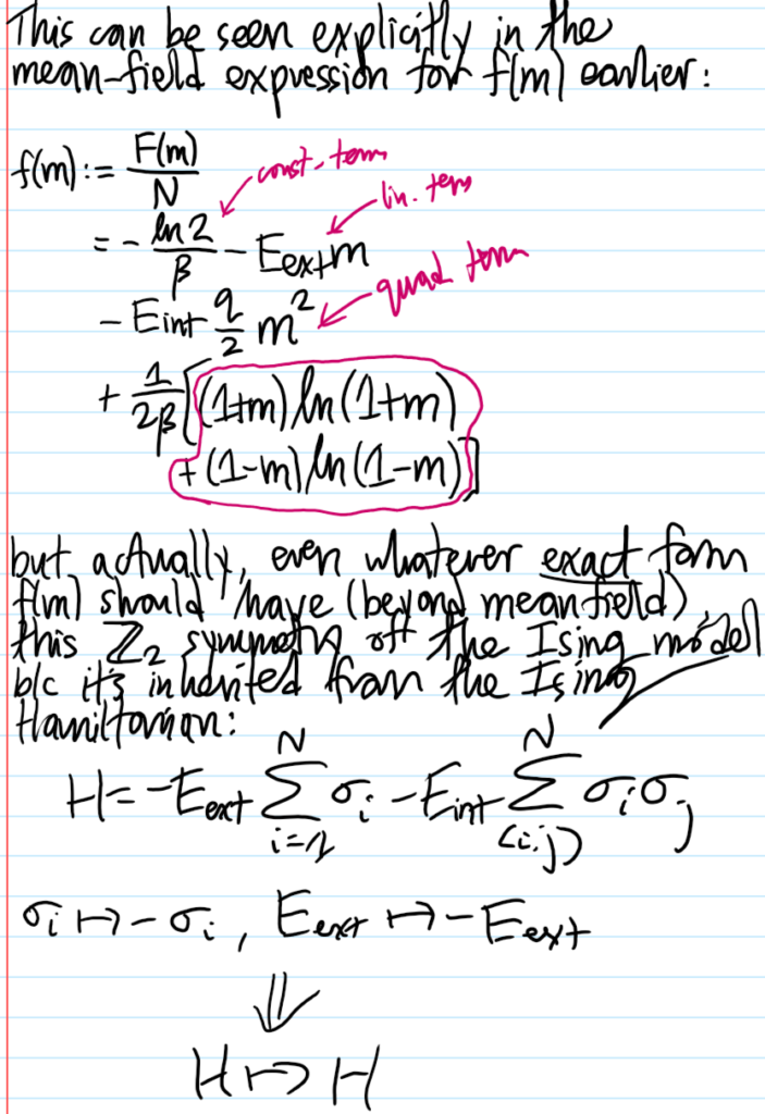
The spontaneous \(\textbf Z_2\) symmetry breaking (i.e. ground state not preserved!) associated to the \(T<T_c\) ordered phase at \(E_{\text{ext}}=0\) is apparent:
Problem #\(8\): In the Ehrenfest classification of phase transitions, an \(N\)-th order phase transition occurs when the \(N\)-th derivative of the free energy \(\frac{\partial^N F}{\partial m^N}\) is discontinuous at some critical value of the order parameter \(m_*\). But considering that \(F=-k_BT\ln Z\) and the partition function \(Z=\sum_{\{\sigma_i\}}e^{-\beta E_{\{\sigma_i\}}}\) is a sum of \(2^N\) analytic exponentials, how can phase transitions be possible?
Solution #\(8\): By analogy, consider the Fourier series for a certain square wave:
\[f(t)=\frac{4}{\pi}\sum_{n=1,3,5,…}^{\infty}\frac{\sin(2\pi n t/T)}{n}\]
Although each sinusoid in the Fourier series is everywhere analytic, the series converges in \(L^2\) norm to a limiting square wave which has discontinuities at \(t_m=mT\), hence not being analytic at those points! So the catch here is that while any finite series of analytic functions (e.g. a partial sum truncation) will have its analyticity preserved, an infinite series need not! This simple result of analysis underpins the existence of phase transitions! In practice of course, for any finite number of spins \(N<\infty\), \(2^N\) will still be finite and in fact there are strictly speaking no phase transitions in any finite system. But in practice \(N\sim 10^{23}\) is so large that it is effectively infinite, and so in this \(N=\infty\) system limit it looks to all intents and purposes as a phase transition.
Similar to the phase transitions, spontaneous symmetry breaking is also an \(N=\infty\) phenomenon only, strictly speaking:
\[m_{SSB}=\lim_{E_{\text{ext}}\to 0}\lim_{N\to\infty}\biggr\langle\frac{1}{N}\sum_{i=1}^N\sigma_i\biggr\rangle\]
where the limits do not commute \(\lim_{E_{\text{ext}}\to 0}\lim_{N\to\infty}\neq\lim_{N\to\infty}\lim_{E_{\text{ext}}\to 0}\) because for any finite \(N<\infty\), \(\langle m\rangle_N=-\frac{1}{N}\frac{\partial F_H}{\partial E_{\text{ext}}}|_{E_{\text{ext}}=0}=0\) since \(\textbf Z_2\) symmetry enforces \(F_H(E_{\text{ext}})=F_H(-E_{\text{ext}})\) so that its derivative must be odd and therefore vanishing at the origin.
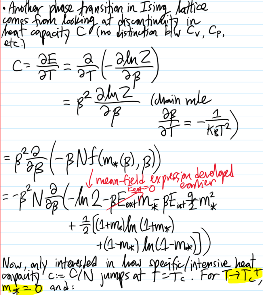
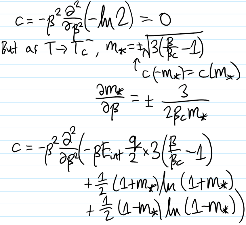
Problem #\(9\): Show that, in the mean-field short-range Ising model at \(E_{\text{ext}}=0\) the specific/intensive heat capacity \(c\) is discontinuous at \(T=T_c\).
Solution #\(9\):
Appendix: Physical Systems Described by Classical Ising Statistics
The purpose of this post is to dive into the intricacies of the classical Ising model. For this, it is useful to imagine the Bravais lattice \(\textbf Z^d\) in \(d\)-dimensions of lattice parameter \(a\), together with a large number \(N\) of neutral spin \(s=1/2\) fermions (e.g. neutrons, ignoring the fact that isolated neutrons are unstable) tightly bound to the lattice sites \(\textbf x\in\textbf Z^d\), each site accommodating at most one fermion by the Pauli exclusion principle. On top of all this, apply a uniform external magnetic field \(\textbf B_{\text{ext}}\) across the entire sample of \(N\) fermions. Physically then, ignoring any kinetic energy or hopping/tunneling between lattice sites (cf. Fermi-Hubbard model), there are two forms of potential energy that contribute to the total Hamiltonian \(H\) of this lattice of spins:
- Each of these \(N\) neutral fermions has a magnetic dipole moment \(\boldsymbol{\mu}_{\textbf S}=\gamma_{\textbf S}\textbf S\) arising from its spin angular momentum \(\textbf S\) (in the case of charged fermions such as electrons \(e^-\), this is just the usual \(\gamma_{\textbf S}=-g_{\textbf S}\mu_B/\hbar\) but for neutrons the origin of such a magnetic dipole moment is more subtle, ultimately arising from its quark structure). This magnetic dipole moment \(\boldsymbol{\mu}_{\textbf S}\) couples with the external magnetic field \(\textbf B_{\text{ext}}\), leading to an interaction energy of the form:
\[V_{\text{ext}}=-\sum_{i=1}^N\boldsymbol{\mu}_{\textbf S,i}\cdot\textbf B_{\text{ext}}=-\gamma_{\textbf S}\sum_{i=1}^N\textbf S_i\cdot\textbf B_{\text{ext}}\]
2. Nearby magnetic dipole moments couple with each other across space, mediating a local internal interaction of the form:
\[V_{\text{int}}=\frac{\mu_0\gamma_{\textbf S}^2}{4\pi}\sum_{1\leq i\neq j\leq N}\frac{3(\textbf S_i\cdot\Delta\hat{\textbf x}_{ij})(\textbf S_j\cdot\Delta\hat{\textbf x}_{ij})-\textbf S_i\cdot\textbf S_j}{|\Delta\textbf x_{ij}|^3}\]
Thus, the total Hamiltonian \(H\) on this state space \(\mathcal H\cong\textbf Z^d\otimes\textbf C^{\otimes 2N}\) is:
\[H=V_{\text{int}}+V_{\text{ext}}\]
Right now, it is hopelessly complicated. From this point onward, a sequence of dubious approximations will be applied to transform this current Hamiltonian \(H\mapsto H_{\text{Ising}}\) to the Ising Hamiltonian \(H_{\text{Ising}}\) (in fact, as mentioned, even the apparently complicated form of the Hamiltonian \(H\) is already approximate; the reason for using neutral fermions is to avoid dealing with an additional Coulomb repulsion contribution to \(H\)).
- Approximation #1: Recall that the direction of the applied magnetic field, say along the \(z\)-axis \(\textbf B_{\text{ext}}=B_{\text{ext}}\hat{\textbf k}\), defines the quantization axis of all the relevant angular momenta. For a sufficiently strong magnetic field \(\textbf B_{\text{ext}}\) (cf. the Paschen-Back effect in atoms), the external coupling \(V_{\text{ext}}\) should dominate the internal coupling \(V_{\text{int}}\) and so all \(N\) spin angular momenta \(\textbf S_i\) will Larmor-precess around \(\textbf B_{\text{ext}}\) with \(m_{s,i}\in\{-1/2,1/2\}\) becoming a good quantum number.
- Approximation #2: Assume that only nearest-neighbour dipolar couplings are important (in \(\textbf Z^d\) there would be \(2d\) nearest neighbours) and that moreover, because all the spins are roughly aligned in the direction of \(\textbf B_{\text{ext}}\), the term \((\textbf S_i\cdot\Delta\hat{\textbf x}_{ij})(\textbf S_j\cdot\Delta\hat{\textbf x}_{ij})\) is not as important as the spin-spin coupling term \(\textbf S_i\cdot\textbf S_j\).
Combining these two approximations, one obtains the Ising Hamiltonian \(H_{\text{Ising}}\) acting on the Ising state space \(\mathcal H_{\text{Ising}}\cong\{-1,1\}^N\):
\[H\approx H_{\text{Ising}}=-E_{\text{int}}\sum_{\langle i,j\rangle}\sigma_i\sigma_j-E_{\text{ext}}\sum_{i=1}^N\sigma_i\]
where \(\sigma_i:=2m_{s,i}\in\{-1,1\}\), \(E_{\text{int}}:=\mu_0\hbar^2\gamma_{\textbf S}^2/16\pi a^3\) is a proxy for the interaction strength between adjacent fermions via the energy gain of being mutually spin-aligned and \(E_{\text{ext}}:=\hbar\gamma_{\textbf S}B_{\text{ext}}/2\) is a proxy for the external field strength via the energy gain of being spin-aligned with it. In the context of magnetism, a material with \(E_{\text{int}}>0\) would be thought of as a ferromagnet while \(E_{\text{int}}<0\) is called an antiferromagnet (this possibility does not arise however after the various approximations that were made). Similarly, \(E_{\text{ext}}\) can be either positive or negative (e.g. for neutrons it is actually negative \(E_{\text{ext}}<0\) because \(\gamma_{\textbf S}<0\)) but for intuition purposes one can just think \(E_{\text{ext}}>0\) so that being spin-aligned with \(\textbf B_{\text{ext}}\) is the desirable state of affairs.
From \(H_{\text{Ising}}\) to \(Z_{\text{Ising}}\)
As usual, once the Hamiltonian \(H_{\text{Ising}}\) has been found (i.e. once the physics has been specified), the rest is just math. In particular, the usual next task is to calculate its canonical partition function \(Z_{\text{Ising}}=\text{Tr}(e^{-\beta H_{\text{Ising}}})\). The calculation of \(Z_{\text{Ising}}\) can be done exactly in dimension \(d=1\) for arbitrary \(E_{\text{ext}}\) (this is what Ising did in his PhD thesis) and also for \(d=2\) provided the absence of an external magnetic field \(E_{\text{ext}}=0\) (this is due to Onsager). In higher dimensions \(d\gg 1\), as the number \(2d\) of nearest neighbours increases, the accuracy of an approximate method for evaluating \(Z_{\text{Ising}}\) known as mean field theory increases accordingly, becoming an exact solution only for the unphysical \(d=\infty\). It is simplest to first work through the mathematics of the mean field theory approach before looking at the special low-dimensional cases \(d=1,(d=2,E_{\text{ext}}=0)\) (it is worth emphasizing that the Ising model can also be trivially solved in any dimension \(d\) if interactions are simply turned off \(E_{\text{int}}=0\) but this would be utterly missing the whole point of the Ising model! edit: in hindsight, maybe not really after all, see the section below on mean field theory).
First, just from inspecting the Hamiltonian \(H_{\text{Ising}}\) it is clear that the net “magnetization” \(\Sigma:=\sum_{i=1}^N\sigma_i\) is conjugate to \(E_{\text{ext}}\), so in the canonical ensemble it fluctuates around the expectation:
\[\langle\Sigma\rangle=-\frac{\partial F_{\text{Ising}}}{\partial E_{\text{ext}}}\]
The ensemble-averaged spin is therefore \(\langle\sigma\rangle=\langle\Sigma\rangle/N\). The usual “proper” way to calculate \(\langle\sigma\rangle\) would be to just directly and analytically evaluate the sums in \(Z_{\text{Ising}}=e^{-\beta F_{\text{Ising}}}\) so in particular \(\langle\sigma\rangle\) shouldn’t appear anywhere until one is explicitly calculating for it. However, using mean field theory, it turns out one will end up with an implicit equation for \(\langle\sigma\rangle\) that can nevertheless still be solved in a self-consistent manner.
To begin, write \(\sigma_i=\langle\sigma\rangle+\delta\sigma_i\) (cf. the Reynolds decomposition used to derive the RANS equations in turbulent fluid mechanics). Then the interaction term in \(H_{\text{Ising}}\) (which is both the all-important term but also the one that makes the problem hard) can be written:
\[V_{\text{int}}=-E_{\text{int}}\sum_{\langle i,j\rangle}(\langle\sigma\rangle+\delta\sigma_i)(\langle\sigma\rangle+\delta\sigma_j)=-E_{\text{int}}\langle\sigma\rangle^2\sum_{\langle i,j\rangle}1-E_{\text{int}}\langle\sigma\rangle\sum_{\langle i,j\rangle}(\delta\sigma_i+\delta\sigma_j)-E_{\text{int}}\sum_{\langle i,j\rangle}\delta\sigma_i\delta\sigma_j\]
Although the variance \(\langle\delta\sigma_i^2\rangle=\langle\sigma_i^2\rangle-\langle\sigma\rangle^2=1-\langle\sigma\rangle^2\) of each individual spin \(\sigma_i\) from the mean background spin \(\langle\sigma\rangle\) is not in general going to be zero (unless of course the entire system is magnetized along or against \(\textbf B_{\text{ext}}\), i.e. \(\langle\sigma\rangle=\pm 1\)), the mean field approximation says that the covariance between distinct neighbouring spins \(\langle i,j\rangle\) should average to \(\sum_{\langle i,j\rangle}\delta\sigma_i\delta\sigma_j\approx 0\), so that, roughly speaking, the overall \(N\times N\) covariance matrix of the spins is not only diagonal but just proportional to the identity \((1-\langle\sigma\rangle^2)1_{N\times N}\).
Thus, reverting back to \(\delta\sigma_i=\sigma_i-\langle\sigma\rangle\) and using for the lattice \(\textbf Z^d\) the identity \(\sum_{\langle i,j\rangle}1\approx Nd\) (because each of \(N\) spins has \(2d\) nearest neighbours but a factor of \(1/2\) is needed to compensate double-counting each bond) and the identity \(\sum_{\langle i,j\rangle}(\sigma_i+\sigma_j)\approx 2d\sum_{i=1}^N\sigma_i\) (just draw a picture), the mean field Ising Hamiltonian \(H’_{\text{Ising}}\) simplifies to:
\[H’_{\text{Ising}}=NdE_{\text{int}}\langle\sigma\rangle^2-E_{\text{ext}}’\sum_{i=1}^N\sigma_i\]
where the constant \(NdE_{\text{int}}\langle\sigma\rangle^2\) doesn’t affect any of the physics (although it will be kept in the calculations below for clarity) and \(E_{\text{ext}}’=E_{\text{ext}}+2dE_{\text{int}}\langle\sigma\rangle\) is the original energy \(E_{\text{ext}}\) together now with a mean field contribution \(2dE_{\text{int}}\langle\sigma\rangle\). This has a straightforward interpretation; one is still acknowledging that only the \(2d\) nearest neighbouring spins can influence a given spin, but now, rather than each one having its own spin \(\sigma_j\), one is assuming that they all exert the same mean field \(\langle\sigma\rangle\) that permeates the entire Ising lattice \(\textbf Z^d\). Basically, the mean field approximation has removed interactions \(E_{\text{int}}’=0\), reducing the problem to a trivial non-interacting one for which it is straightforward to calculate (this is just repeating the usual steps of calculating, e.g. the Schottky anomaly):
\[Z’_{\text{Ising}}=(2e^{dE_{\text{int}}\langle\sigma\rangle^2}\cosh\beta E’_{\text{ext}})^N\]
\[F’_{\text{Ising}}=-\frac{N}{\beta}(\ln\cosh\beta E’_{\text{ext}}+dE_{\text{int}}\langle\sigma\rangle^2+\ln 2)\]
\[\langle\sigma\rangle=\tanh\beta E’_{\text{ext}}=\tanh\beta(E_{\text{ext}}+2dE_{\text{int}}\langle\sigma\rangle)\]
As promised earlier, this is an implicit equation for the average spin \(\langle\sigma\rangle\) that can, for a fixed dimension \(d\), be solved for various values of temperature \(\beta\) (which intuitively wants to randomize the spins) and energies \(E_{\text{int}},E_{\text{ext}}\) (both of which intuitively want to align the spins). The outcome of this competition is the following:
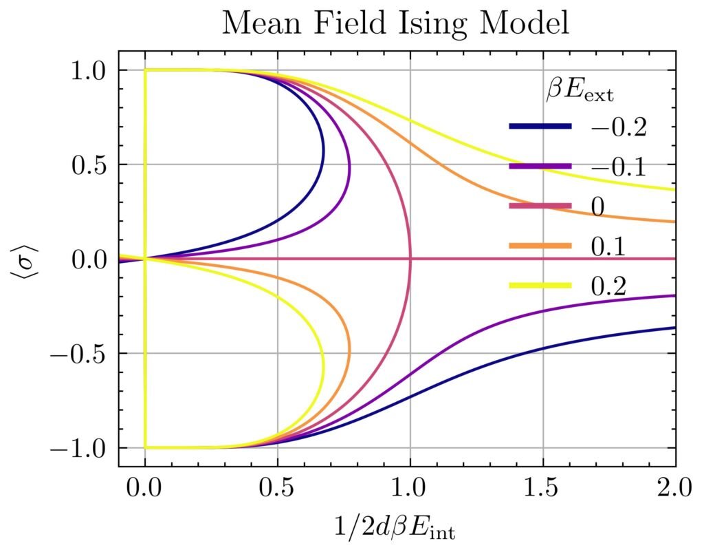
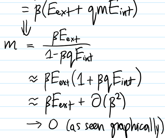
If one applies any kind of external magnetic field \(E_{\text{ext}}\neq 0\), then as one increases the temperature \(1/2d\beta E_{\text{int}}\to\infty\), the mean spin \(\langle\sigma\rangle\to 0\) randomizes gradually (more precisely, as \(\langle\sigma\rangle=\beta E_{\text{ext}}+2dE_{\text{int}}E_{\text{ext}}\beta^2+O_{\beta\to 0}(\beta^3)\)). The surprise though occurs in the absence of any external magnetic field \(E_{\text{ext}}=0\); here, driven solely by mean field interactions, the mean spin \(\langle\sigma\rangle=0\) abruptly vanishes at all temperatures \(T\geq T_c\) exceeding a critical temperature \(kT_c=2dE_{\text{int}}\). This is a second-order ferromagnetic-to-paramagnetic phase transition (it is second order because the discontinuity occurs in the derivative of \(\langle\sigma\rangle\) which itself is already a derivative of the free energy \(F’_{\text{Ising}}\)). Meanwhile, there is also a first-order phase transition given by fixing a subcritical temperature \(T<T_c\) and varying \(E_{\text{ext}}\), as in this case it is the mean magnetization \(\langle\sigma\rangle\) itself that jumps discontinuously.
Note also that, similar to the situation for the Van der Waals equation when one had \(T<T_c\), here it is apparent that at sufficiently low temperatures for arbitrary \(E_{\text{ext}}\), the mean field Ising model predicts \(3\) possible mean magnetizations \(\langle\sigma\rangle\). For \(E_{\text{ext}}=0\), the unmagnetized solution \(\langle\sigma\rangle=0\) solution turns out to be an unstable equilibrium. For \(E_{\text{ext}}>0\), the solution on the top branch with \(\langle\sigma\rangle>0\) aligned with the external magnetic field is stable while among the two solutions with \(\langle\sigma\rangle<0\), one is likewise unstable while one is metastable, and similarly for \(E_{\text{ext}}<0\).
Critical Exponents
Solving The Ising Chain (\(d=1\)) Via Transfer Matrices
Low & High-\(T\) Limits of Ising Model in \(d=2\) Dimensions
Talk about Peierls droplet, prove Kramers-Wannier duality between the low and high-\(T\) regimes.
Beyond Ferromagnetism
The point of the Ising model isn’t really to be some kind of accurate model for any real-life physical system, but just a “proof of concept” demonstration that phase transitions can arise from statistical mechanics; although the sum of finitely many analytic functions is analytic, in the thermodynamic limit a phase transition can appear. Similar vein of mathematical modelling can be used to model lattice gases,
Talk about the Metropolis-Hastings algorithm.
