
Problem: What does it mean to say that a field \(\mathbf E(\mathbf x,t)\in\mathbf C^3\) is a plane wave with speed \(c\geq 0\) in direction \(\hat{\mathbf z}\in S^2\)? Show that a general such plane wave can be written as a Fourier synthesis over all frequencies \(\omega\in\mathbf R\):
\[\mathbf E(z,t)=\int_{-\infty}^{\infty}d\omega\left(\mathbf E_+(\omega)e^{ik_{\omega}(z-ct)}+\mathbf E_-(\omega)e^{ik_{\omega}(z+ct)}\right)\]
where \(k_{\omega}:=\omega/c\). In the special case where \(\mathbf E(\mathbf x,t)\) is the electric field of an electromagnetic wave in vacuum, what additional constraints on the Fourier components \(\mathbf E_{\pm}(\omega)\) are present? Under what further assumptions can the description of the plane wave be reduced to a Jones vector \(\mathbf E_0\in\mathbf C^2\)?
Solution: The “plane” part means that \(\mathbf E(\mathbf x,t)=\mathbf E(z,t)\) is constant on planes of constant \(z:=\mathbf x\cdot\hat{\mathbf z}\) perpendicular to \(\hat{\mathbf z}\). The “wave” part means that \(\mathbf E(z,t)=\mathbf E_+(z-ct)+\mathbf E_-(z+ct)\) satisfies the dispersionless wave equation with speed \(c=\omega/k\). Each of these travelling plane wave components can be Fourier expanded which leads to the desired result. It is essential to emphasize that all Fourier components \(\omega\in\mathbf R\) are travelling either parallel/anti-parallel to \(\hat{\mathbf z}\) in the Fourier superposition, i.e. \(\partial\hat{\mathbf z}/\partial\omega=\mathbf 0\).
For electromagnetic plane waves, \(\frac{\partial}{\partial\mathbf x}\cdot\mathbf E=0\Rightarrow\mathbf k\cdot\mathbf E=\hat{\mathbf z}\cdot\mathbf E=0\) so both \(\mathbf E_{\pm}(z\pm ct)\) vectors are confined to lie within their own contour planes.
Finally, in order to be amenable to a Jones vector description, one has to assume the plane wave is travelling so that e.g. \(\mathbf E_-=\mathbf 0\) and monochromatic so that the surviving Fourier component is of the form \(\mathbf E_+(\omega’)=\mathbf E_0\delta(\omega’-\omega)\); then \(\mathbf E_0\in\mathbf C^2\) is the Jones vector of this travelling, monochromatic electromagnetic plane wave:
\[\mathbf E(z,t)=\mathbf E_0e^{i(kz-\omega t)}\]
(there exists a more general formalism known as Mueller calculus that extends the Jones calculus to deal with more general kinds of plane waves). Sometimes, the Jones vector is normalized \(\mathbf E_0\mapsto\mathbf E_0/|\mathbf E_0|\) to live on the “Bloch sphere” (see Poincare sphere) but this discards irradiance information \(\langle I\rangle=\varepsilon_0c|\mathbf E_0|^2/2\).
Problem: State the Jones vectors for travelling, monochromatic EM plane waves with:
a) Elliptical polarization
b) Circular polarization
c) Linear polarization at an angle \(\theta\) to the \(x\)-axis
Solution:
a) This is just the most general Jones vector \((E_x,E_ye^{i\phi})\) for (in general distinct) amplitudes \(E_x,E_y\in\mathbf R\) separated by an arbitrary phase \(e^{i\phi}\in U(1)\). Thus, just to emphasize again: Jones vector\(\Leftrightarrow\)Elliptic polarization. They are synonyms! Defining \(\tan\psi:=E_y/E_x\), the semi-major axis of this ellipse will be tilted relative to the \(x\)-axis at an angle \(\theta\) given by \(\tan 2\theta=\tan 2\psi\cos\phi\).
b) This is the special case of elliptical polarization where \(2\) conditions are simultaneously true: \(E_x=E_y:=E_0/\sqrt{2}\) and \(\phi=\pm\pi/2\). In that case, the Jones vector reduces to \(\mathbf E_0=\frac{E_0}{\sqrt 2}(1,\pm i)\) where the \(\pm\) distinguishes between left vs. right circular polarization.
c) This is the special case of elliptical polarization where \(\phi\in\{0,\pi\}\). Thus, one can write \(E_x=E_0\cos\theta\) and \(E_y=E_0\sin\theta\) so that a linearly polarized Jones vector is of the form \(\mathbf E_0=E_0(\cos\theta,\sin\theta)\).
Problem: What does it mean for a (possibly nonlinear) dielectric to be birefringent? What fundamentally causes birefringence? How is birefringence typically quantified?
Solution: Recall that \(\mathbf D:=\varepsilon_0\mathbf E+\mathbf P\) where the polarization \(\mathbf P=\mathbf P(\mathbf E)\) induced by \(\mathbf E\) may in general (for a generic, nonlinear dielectric which may be piezoelectric or even pyroelectric or even ferroelectric) be expanded as a Taylor series about \(\mathbf E=\mathbf 0\) of the form:
\[\mathbf P=\mathbf P_0+\varepsilon_0(\chi^{(1)}\mathbf E+\chi^{(2)}\mathbf E^{\otimes 2}+\chi^{(3)}\mathbf E^{\otimes 3}+…)\]
so that one can write \(\mathbf D=\varepsilon\mathbf E+\mathbf P_0\) with (effective) permittivity tensor \(\varepsilon:=\varepsilon_0(1+\chi^{(1)}+\chi^{(2)}\mathbf E+\chi^{(3)}\mathbf E^{\otimes 2}+…)\). The dielectric is then said to be birefringent iff its permittivity tensor \(\varepsilon\) is anisotropic (i.e. possesses at least \(2\) distinct permittivity eigenvalues). If \(2\) of the \(3\) permittivity eigenvalues are the same \(\varepsilon_1=\varepsilon_2\neq\varepsilon_3\), then the dielectric is said to be uniaxially birefringent with \(\varepsilon_1,\varepsilon_3\) referred to respectively as the ordinary and extraordinary permittivities (and the principal axis associated to \(\varepsilon_3\) being referred to as the optic axis). If instead all \(3\) permittivity eigenvalues are distinct, then the dielectric is said to be biaxially birefringent. Fundamentally, these forms of optical anisotropy are either due to structural anisotropy in the lattice of nuclei themselves (which may be intrinsic or induced by external stress for instance), or anisotropy in the electron cloud distribution induced by the light itself even if the lattice itself is e.g. primitive cubic and hence isotropic. In any case, the key corollary of birefringence is that \(\mathbf D\) need not be parallel to \(\mathbf E\). In particular, for an electromagnetic wave propagating in direction \(\mathbf k\), one has the orthogonal triad \((\mathbf D,\mathbf H,\mathbf k)\). But this means the Poynting field \(\mathbf I=\mathbf E\times\mathbf H\) need not be parallel to \(\mathbf k\).
Provided that \(\varepsilon^{\dagger}=\varepsilon\) is Hermitian (which will be the case iff there is no energy transfer between the light and the dielectric in the form of stimulated absorption or emission), one can always diagonalize it in an orthonormal eigenbasis of real permittivity eigenvalues \(\varepsilon_1,\varepsilon_2,\varepsilon_3\in\mathbf R\). It is thus convenient to consider a retardation ellipsoid in \(\mathbf D\)-space (cf. Poinsot’s ellipsoid in \(\mathbf L\)-space) defined by the effective electric energy density \(D^2/2\varepsilon_{\text{eff}}\) as if the dielectric were isotropic with scalar permittivity \(\varepsilon_{\text{eff}}\):
\[\frac{D_1^2}{2\varepsilon_1}+\frac{D_2^2}{2\varepsilon_2}+\frac{D_3^2}{2\varepsilon_3}=\frac{D^2}{2\varepsilon_{\text{eff}}}\]
Consider the specific case \(\varepsilon_1=\varepsilon_2\) of a uniaxially birefringent dielectric, and suppose \(\mathbf k=k(\sin\theta,0,\cos\theta)\) is incident at some angle \(\theta\) (w.l.o.g. \(\phi:=0\)) to its optic axis. Since \(\mathbf k\cdot\mathbf D=0\), a generic electric displacement \(\mathbf D\) can be decomposed in the orthonormal basis \((0,1,0),(-\cos\theta,0,\sin\theta)\) of that degenerate subspace and its components evolved independently. Thus, w.l.o.g. one can separately consider the ordinary case \(\mathbf D=D(0,1,0)\) and the extraordinary case \(\mathbf D=D(-\cos\theta,0,\sin\theta)\). In the ordinary case, plugging into the retardation ellipsoid, one obtains \(\varepsilon_{\text{eff}}=\varepsilon_1\), whereas in the extraordinary case one obtains \(1/\varepsilon_{\text{eff}}(\theta)=\cos^2\theta/\varepsilon_1+\sin^2\theta/\varepsilon_3\).
For dielectrics described by a centrosymmetric crystal structure so that the induced polarization \(\mathbf P(-\mathbf E)=-\mathbf P(\mathbf E)\) is an odd function of the applied \(\mathbf E\)-field, both the spontaneous polarization \(\mathbf P_0=\mathbf 0\) and Pockel’s electric susceptibility tensor \(\chi^{(2)}=0\) vanish.
Birefringence is fundamentally a measure of (a.k.a. is caused by) symmetry breaking. This could be due to tetragonal or orthorhombic lattice in a solid, or molecular chirality. One can also consider a kind of birefringence in conductors where \(\varepsilon(\omega)=\varepsilon_0+i\sigma(\omega)/\omega\) if the conductivity tensor \(\sigma\) is anisotropic.
Problem: Write down the Jones matrices for:
a) Linear polarizer (e.g. a dichroic Polaroid film) at angle \(\theta\) to the \(x\)-axis. Check the cases \(\theta=0,\pi/2\) and prove Malus’s law.
b) A \(\phi\)-waveplate with fast axis at angle \(\theta\) to the incident polarization vector. What about the special cases of a \(\lambda/4\)-waveplate and a \(\lambda/2\)-waveplate?
c) Crossed linear polarizers.
d) A cuvette containing chiral sugar water (e.g. dextrose) of length \(\ell\), with circular birefringence \(\Delta n:=n_{\text{left}}-n_{\text{right}}\) (aka optical activity).
Solution:
a) The eigenvectors of this Jones matrix must be \((\cos\theta,\sin\theta)\) and \((-\sin\theta,\cos\theta)\), both with respective eigenvalues \(1\) and \(0\). Thus, in analogy with quantum mechanical formulas like \(H=\sum_EE|E\rangle\langle E|\), one has:
\[1\begin{pmatrix}\cos\theta \\ \sin\theta\end{pmatrix}^{\otimes 2}+0\begin{pmatrix}-\sin\theta \\ \cos\theta\end{pmatrix}^{\otimes 2}=\begin{pmatrix}\cos^2\theta&\cos\theta\sin\theta \\ \cos\theta\sin\theta & \sin^2\theta\end{pmatrix}\]
In particular, this is \(\begin{pmatrix}1&0\\0&0\end{pmatrix}\) for \(\theta=0\) and \(\begin{pmatrix}0&0\\0&1\end{pmatrix}\) for \(\theta=\pi/2\) as expected.
A travelling monochromatic plane wave polarized with Jones vector \(E_0(1,0)\) along the \(x\)-axis maps to \(E_0(\cos^2\theta,\cos\theta\sin\theta)\) which is associated to the time-averaged intensity \(\langle I\rangle=\varepsilon_0 cE_0^2(\cos^4\theta+\cos^2\theta\sin^2\theta)/2=\langle I_0\rangle\cos^2\theta\) where \(\langle I_0\rangle=\varepsilon_0 cE_0^2/2\).
b) The eigenvectors \((\cos\theta,\sin\theta)\) and \((-\sin\theta,\cos\theta)\) are the same as for the linear polarizer tilted at \(\theta\) but the respective eigenvalues are now \(1\) and \(e^{i\phi}\) with \(\phi:=k\Delta n\ell\) for vacuum wavenumber \(k:=\omega/c\), (uniaxial or biaxial) birefringence \(\Delta n:=n_{\text{slow}}-n_{\text{fast}}\), and waveplate thickness \(\ell\). Thus, the Jones matrix is:
\[1\begin{pmatrix}\cos\theta \\ \sin\theta\end{pmatrix}^{\otimes 2}+e^{i\phi}\begin{pmatrix}-\sin\theta \\ \cos\theta\end{pmatrix}^{\otimes 2}=\begin{pmatrix}\cos^2\theta+e^{i\phi}\sin^2\theta &\cos\theta\sin\theta (1-e^{i\phi}) \\ \cos\theta\sin\theta (1-e^{i\phi}) & \sin^2\theta + e^{i\phi}\cos^2\theta\end{pmatrix}\]
For a \(\Delta n\ell:=\lambda/4\)-waveplate, \(\phi=\pi/2\) so \(e^{i\phi}=i\):
\[\begin{pmatrix}\cos^2\theta+i\sin^2\theta &\cos\theta\sin\theta (1-i) \\ \cos\theta\sin\theta (1-i) & \sin^2\theta + i\cos^2\theta\end{pmatrix}\]
For \(\Delta n\ell:=\lambda/2\)-waveplate, \(\phi=\pi\) so \(e^{i\phi}=-1\):
\[\begin{pmatrix}\cos 2\theta & \sin 2\theta \\ \sin 2\theta & \cos 2\theta\end{pmatrix}\]
c) Zero of course.
d) Essentially identical eigenvalues \(1,e^{i\phi}\) as the waveplate (where \(\phi=k\Delta n\ell\) still holds just with a re-interpretation of \(\Delta n\) and \(\ell\)), only the eigenvectors change to left/right circularly polarized normalized Jones vectors \((1,\pm i)/\sqrt{2}\):
\[1\begin{pmatrix}1/\sqrt{2} \\ i/\sqrt{2}\end{pmatrix}^{\otimes 2}+e^{i\phi}\begin{pmatrix}1/\sqrt{2} \\ -i/\sqrt{2}\end{pmatrix}^{\otimes 2}=e^{i\phi/2}\begin{pmatrix}\cos\phi/2 & \sin\phi/2 \\ \sin\phi/2 & -\cos\phi/2\end{pmatrix}\]
Thus, the plane of linear polarization (which is an equal amplitude superposition of left and right circular polarizations) is rotated by \(\phi/2\), or equivalently \(\partial(\phi/2)/\partial\ell=k\Delta n\) is the specific rotation power of the sugar solution which can either be positive or negative depending on whether \(\Delta n>0\) is dextrorotatory or \(\Delta n<0\) is levorotatory.
(aside: even in intrinsically achiral media, one can induce chirality by applying an uniform external magnetic field \(\mathbf B\) to a dielectric or plasma; this magnetically-induced circular birefringence is known as the Faraday effect \(\phi/2=VB\ell\) where \(V=V(\omega)\) is called the Verdet constant).
Optical Fibers & APC Connectors
An optical fiber is a waveguide for light waves. The idea is to use it to transmit light over long distances with minimal loss. It consists of an inner core, made of glass or plastic, where total internal reflection can take place within the waveguide (ignoring evanescent transmitted waves) because of a cladding with (higher/lower?) refractive index, and a jacket (blue layer in the picture).
At the ends of optical fibers, one typically also has angled physical contact (APC) connectors to minimize back-reflection of light (by using an angled design usually around \(8^{\circ}\)). These ensure alignment of optical fiber cores when connecting two optical fibers to each other.
Often, optical fibers can be polarization-maintaining (PM) meaning that when one excites a given optical fiber. This is because apparently the core of an optical fiber is typically already pre-stressed to give it some kind of birefringence \(\Delta n=n_{\text{slow}}-n_{\text{fast}}\) (general rule of thumb: any symmetry which is easily broken will be broken; for example the magnetic field is never actually \(\textbf B=\textbf 0\) due to Earth, someone’s phone, etc. and since you don’t want other things to be defining your quantization axis, so you should just apply a magnetic field yourself anyways).
Coupling Laser Light into an Optical Fiber
Goal is to get laser beam to be normally incident \(\theta_x=\theta_y=0\) at the center \(x=y=0\) of an optical fiber. Although initially this sounds quite trivial, as with any waveguide, the optical fiber is extraordinarily sensitive to any small deviations in these \(4\) degrees of freedom \(x,y,\theta_x,\theta_y\) and will only work if these \(4\) conditions are almost perfectly met (hence rendering the task highly non-trivial). Thus, the naive solution of just trying to align the laser beam into the optical fiber “by hand” is hopeless since one’s hands afford merely coarse control over \(x,y,\theta_x,\theta_y\) but clearly here one requires much finer control in order to successfully couple the laser light into the optical fiber.
The way to obtain such fine control is to use mirrors; each mirror comes with fine control in both spherical coordinates \(\phi,\theta\) (and also there is leeway in exactly where the laser is incident on the mirror and the fact that it need not be exactly \(45^{\circ}\) or anything like that). Of course changing the azimuth \(\phi\) of a given mirror will simultaneously change both \(x,\theta_x\) and similarly changing the zenith angle \(\theta\) of a mirror simultaneously affects both \(y,\theta_y\), so in this sense these degrees of freedom are “coupled”. Specifically, each mirror provides for \(2\) degrees of freedom \(\phi,\theta\) which is why in total \(2\) mirrors are actually needed to properly couple the laser into the optical fiber.
One can connect the output end of the optical fiber to a fiber pen and use a translucent polymer sheet to see where the laser beam from the laser intersects the laser beam from the fiber pen at various regions in the setup. From having played around with the setup, it is more sensible to focus on aligning them at the extremes of the path, which tends to automatically ensure that they will be aligned everywhere else in the middle. Moreover, a general rule of thumb turns out to be that in order to align a section, the mirror one should do fine adjustments is, perhaps counterintuitively, the one further away (is there some name for this kind of algorithm?). Doing it iteratively like this will converge onto an aligned optical system; doing it the other way will diverge into a hopelessly misaligned system.
After having completed the “fine structure” alignment of the mirrors properly so that there is for sure some non-zero signal coming out the output of the optical fiber, one can then proceed to a “hyperfine” level of adjustments, putting the output of the optical fiber into a photodiode and measuring the photocurrent developed across a potentiometer \(R\) via a multimeter, or just directly using a power meter. Here again, one essentially seeks to maximize the photodiode signal by an algorithm which vaguely feels like a manual implementation of gradient descent. More precisely, it turns out to be more advisable to make some small random perturbation to the \(\phi\) (resp. \(\theta\)) of the mirror farther away (not necessarily physically, but in the sense of the optical path length) from the input of the optical fiber, then adjusting \(\phi\) (resp. \(\theta\)) of the mirror closer to the optical fiber input until the signal is locally maximized, and repeating this until one eventually converges onto not merely a local, but global maximum (2D search). Finally, also consider the focal length of the lens relative to the fiber (this is a 1D search at the end). At this point, one can feel pretty confident that the laser light is properly coupled into the optical fiber, i.e. that \(x\approx y\approx\theta_x\approx\theta_y\approx 0\). Each time one takes a fiber out and puts it back in again, one has to recouple because of how sensitive the whole alignment is.
Optical Tables & Breadboards
Small vibrations (e.g. footsteps, motors, etc.) can perturb the delicate alignment of optical systems, hence all optical components need to be firmly bolted down to an optical table (possibly with the aid of ferromagnetic bases). The top and bottom layers of an optical table are usually manufactured from some grade of stainless steel perforated by a square lattice of \(\text{M}6\) threaded holes with lattice parameter \(\Delta x=25\text{ mm}\) (recall that \(\text{M}D\times L\) is the standard notation for a metric thread of outer diameter \(D\text{ mm}\) and length \(L\text{ mm}\) and typically one assumes the thread pitch \(\delta\text{ mm}\) is the coarsest/largest one that is standardized for that particular thread diameter \(D\) so that the helix winds \(N=L/\delta\) times around, although \(\delta\) could be finer/smaller too, see this reference). The exact engineering details of how an optical table seeks to critically damp external vibrations is interesting, involving the use of pneumatic legs and several layers of viscoelastic materials sandwiched between the steel layers in a rigid honeycomb structure.

Optical breadboards are basically just smaller, less fancy version of an optical table, mainly used for prototyping and easier portability of a particular modular setup into some main optical table.
Acousto-Optic Modulators (AOMs)
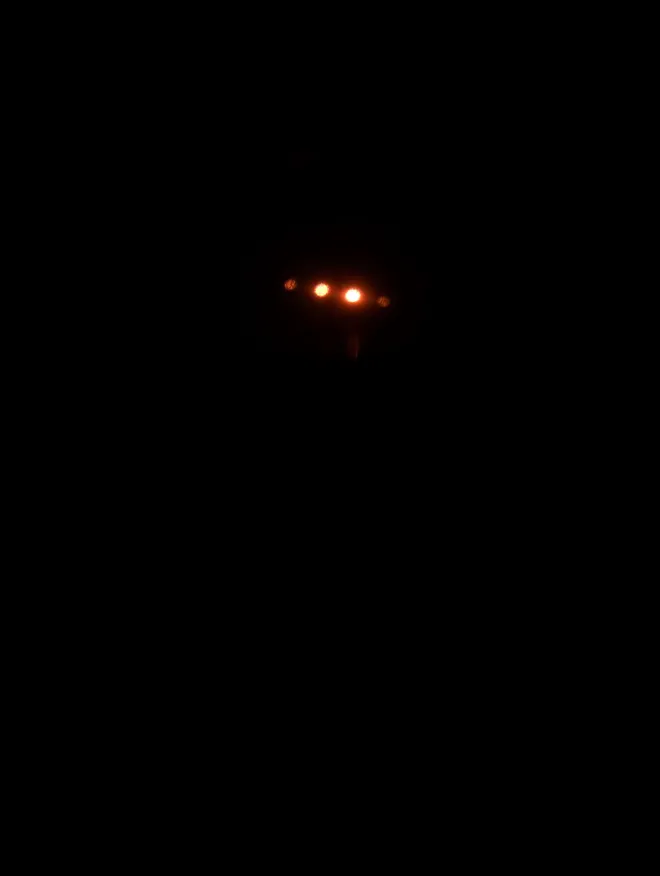
An acousto-optic modulator (AOM), also known as an acousto-optic deflector (AOD), is at first glance similar to a diffraction grating for light in the sense that if one shines some incident plane wave from a laser through the hole in the AOM, then out comes an \(m=0\) order mode in addition to \(m=\pm 1\) and occasionally higher-order modes too (the exact distribution of intensities among these harmonics will depend very sensitively on the incident angle that one shines the laser light at into the AOM).
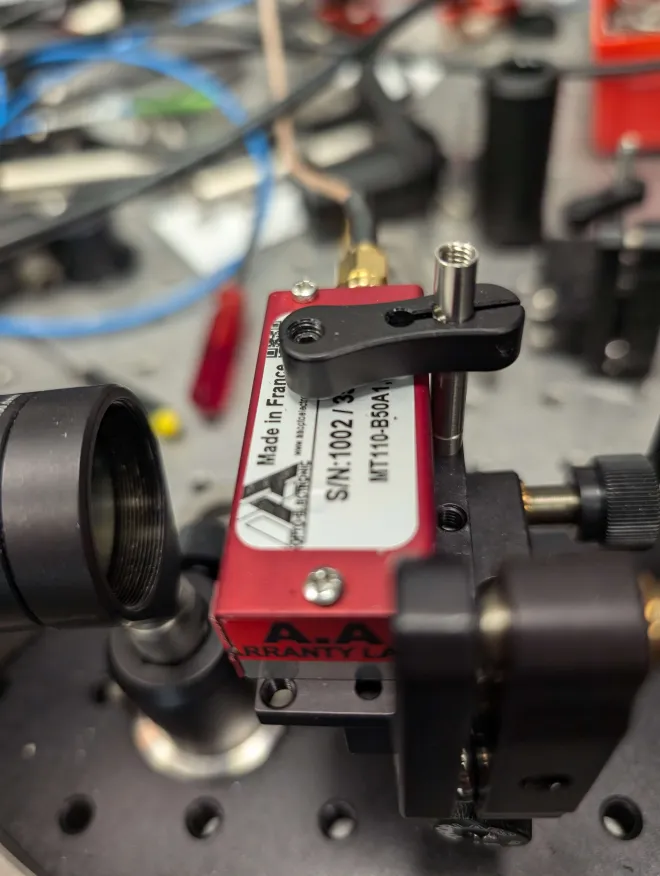
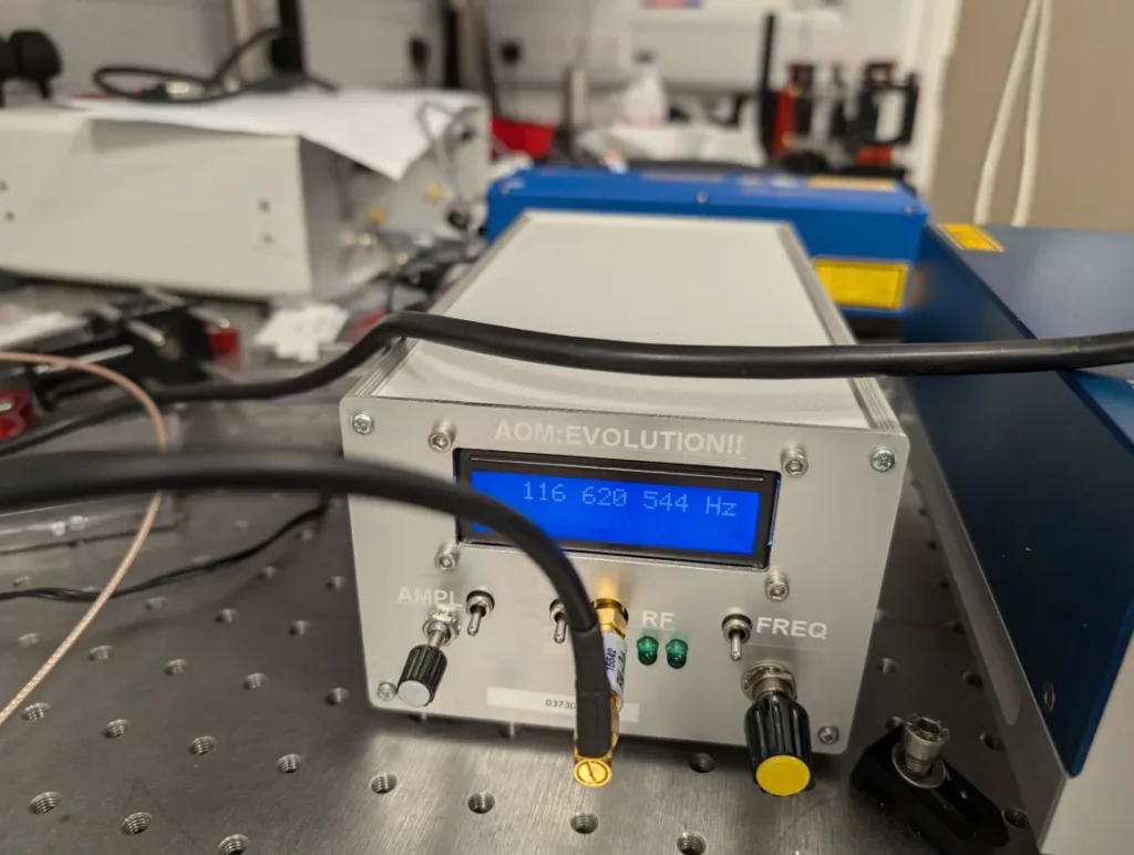
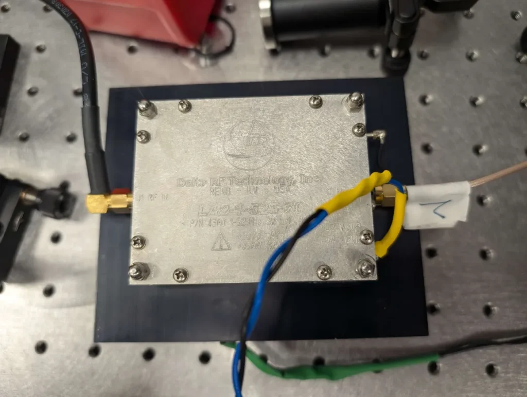
However, despite being superficially similar to a diffraction grating, there are some notable differences; the first is that the Fraunhofer interference pattern of a diffraction grating typically occurs via a (\(2\)-dimensional) screen with a bunch of slits on it; here a (\(3\)-dimensional!) volume Bragg grating (VBG) is used instead, which in practice means some kind of glass attached to a piezoelectric transducer that drives the glass (i.e. applies periodic stress to it) at some radio frequency \(f_{\text{ext}}\sim 100\text{ MHz}\) via an external RF driver. This induces a periodic modulation in the glass’s refractive index \(n=n(x)\) where the “period” \(\lambda_{\text{ext}}=c_{\text{glass}}/f_{\text{ext}}\) over which \(n(x+\lambda_{\text{ext}})=n(x)\) corresponds to the wavelength of the sound waves, where \(c_{\text{glass}}\) is the phase velocity of sound waves in the glass.
Provided the light is incident at the Bragg angle \(\theta_B\approx\sin\theta_B\approx 2\lambda/\lambda_{\text{ext}}\), then one has an effective crystal with interplanar spacing \(\lambda_{\text{ext}}\) and so the Bragg condition yields the angular positions of the constructive maxima of the Brillouin scattering:
\[2\lambda_{\text{ext}}\sin\theta_m=m\lambda\]
In addition, whereas for ordinary light incident on a diffraction grating the wavelength and frequency don’t change after diffraction, here because the photons either absorb or emit a phonon quasiparticle (respectively \(m=\pm 1\) orders), they do also accrue a slight Doppler shift in the frequency. When an AOM is labelled as being \(110\text{ MHz}\) for instance, it does not mean that the only Doppler shifts it is able to provide are exactly \(\pm 110\text{ MHz}\) but rather the diffraction efficiency \(\eta\) is greatest at this frequency, with some FWHM bandwidth \(\delta f_{\text{ext}}\) around this. For instance, for \(2\) AOMs in the lab, the following frequency response efficiency curves were measured (for both single pass and double pass, the latter of which should roughly be the square of the former).
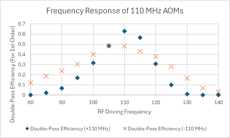
AOMs are commonly used in a double-pass configuration, which means that light is passed through, then passed back again in exactly along the trajectory it came. If the diffraction efficiency of the first-order is \(\eta(\omega)<1\) at some frequency \(\omega=2\pi f\) ideally around the central \(\omega\) of the AOM (e.g. \(\omega=2\pi\times 110\text{ MHz}\)), then double-passing will lead to a reduced frequency \(\eta^2(\omega)<\eta(\omega)\). Provided one picks out the right order (not always trivial to do, need to change the driving amplitude to see which order drops faster, and use geometrical ray optics arguments), then this allows accruing a Doppler shift of \(2f_{\text{ext}}\) without sacrificing too much efficiency (if tried to get this from the \(m=2\) mode on a single-pass, would lose a lot of efficiency). AOMs are also commonly used for Q-switching in lasers (i.e. as glorified switches b/c they can switch on nanosecond time scales).
Laser (Toptica) with massive DLC Pro driver? Talk about how lasers work + lasing requirements
Notes on how Zoran’s lab works:
- The UHV in the MOT and science cells are like \(10^{-11},10^{-13}\text{ mbar}\) respectively, measured by a current which is on the order of \(\text{nA}\) (but at such low pressures, with such few particles, one can argue that pressure fails to even be a well-defined quantity).
- There are \(4\) AOM drivers for D1 cooling/repump and D2 cooling/repump light. Each has frequency, TTL, and amplitude control which need to be connected to analog channels like AO1, AO2, etc. which in turn are controlled in Cicero.
- Laser goggles have certain wavelength ranges over which they block best. The ODT uses 767 nm red light, but the box trap uses 532 nm green light.
- The Toptica laser controller is one component of a PID control loop.
- First, saturated absorption spectroscopy (require heat b/c K-39 to be in a gaseous form b/c otherwise just K-39 liquid/solid sitting at the bottom of the tube; this is achieved by winding some coils around and passing large current through coils and relying on resultant Joule heating; for K-39 need around human body temperature? \(35-40^{\circ}\text{ C}\) (the double-pass thing in the absorption cell) is used to get a Doppler-free \(\lambda_{D1},\lambda_{D2}\) signals that are fed to photodiodes, which send this to the Toptica laser controller which sends it to the Toptica software that’s used for laser locking.
- Need to lock the laser b/c a piezoelectric crystal has some voltage applied to it that causes mechanical deformation, move distance b/w 2 mirrors, but overtime it can drift due to temperature fluctuations, etc.
- The photodiodes need to be powered (by old car battery in this case) and also a separate cable which feeds into Toptica laser controller (it is also this cable which has the extra resistor at its end…I think idea is that the photodiode converts absorption signal into a photocurrent that flows across the resistor, and gets converted into a voltage…note that it’s a BNC cable, and most BNC cables already have some internal resistance, so this resistor really is just an extra resistor which I guess is to decrease the “gain” in some sense?).
- Kibble-Zurek mechanism?
- Anything in the lab (e.g. PCs, soldering irons, vacuum pumps, all kettle plugs, etc.) connected to AC mains needs to be PAT tested.
- There are \(4\) sets of coils in the experiment. In chronological order of use, they are:
- Quadrupole field coils (both \(x\),\(y\) and \(z\)) for the MOT and magnetic trapping.
- Guide field coils (to impose a quantization axis?) on MOT side for pumping and on the imaging side.
- Feshbach (“Fesh”) field coils for the science cell (to exploit Feshbach resonance of hyperfine states in order to tune s-wave scattering length).
- Compensation coils in \(x,y,z\) (the \(z\) compensation coil is also called “anti-\(g\)” coil for obvious reasons).
- Speedy coils? For quantum quench experiments?
- One of the coils cancels the curvature in the Feshbach coils.
- Each of these coils obviously requires a very bulky power supply.
- Igor’s thesis should contain more information about the coils.
- The track (arm which moves the magnetically trapped atoms) has \(3\) states, START, MOVE, MOVE2, and ENERGIZE? There is a track control box connected to the analog channels which one can use to control how the track moves in Cicero during an experimental sequence.
- Regarding water cooling of the experiment, the water is already pressurized, so adding a pump would only slow it down?
- The pipes also contain flow meters which monitor the flow rate \(|\textbf v|\) of the water (not sure how?), and send this information to a logic circuit which also uses temperature control. Will suddenly stop all current flowing through Feshbach coils if it detects that some thresholds are breached on both; thus, behaves as a current-controlled switch, aka a transistor, and more precisely they are IGBTs (insulated-gate bipolar transistor) because it turns out only these transistors are rated for the kinds of currents being used here.
- For all the coils, one frequently would like to switch them off suddenly. If you just do this directly, the significant inductance \(L\) of the coils will lead to a substantial back emf that would destroy the PSU. Hence the need for an alternative path for current to flow, which is why we also have a capacitor in parallel?
- Apparently, the light inside an optical fiber can also heat the fiber enough to melt it…
- There can be up to \(I\sim 200\text{ A}\) of current flowing through the Feshbach coils, with \(V=400\text{ V}\)…the whole circuit is low-resistance so if you touch probably not lethal but still better to be safe. The
The D1, D2 cooling and repump light must first get the required frequency shifts, then it all gets coupled simultaneously into a TA (amplifier) which should be seeded at all times, is externally controlled by a current knob \(I\) that dictates how much amplification \(A=A(I)\) it gives to the laser power. This is all then coupled into a polarization-maintaining optical fiber that goes into an optical fiber port cluster (FPC) (see the ChatGPT blurb about it) which is basically a compact setup of mirrors/lenses/polarizing beamsplitters (Chris says conceptually it’s not hard to build one yourself, just that save time with a company at the cost of double the price cf. self-building; similar remarks even apply to e.g. a laser which can be self-built and indeed many labs do that, just takes time). This then takes the incident light from the fiber and redistributes it into \(6\) beams of roughly equal power for the MOT (i.e. the “O” in “MOT”).
The MOT loading time \(\Delta t_{\text{load}}\) is the time to load the MOT from the vapor of K-39 atoms that sits at some background pressure \(p_o\) and temperature \(T_0\). Some exponential “charging curve” \(1-e^{-t/t_{\text{load}}}\)? And also, normally you gauge how well the MOT is working (and decide when need to fire again) by measuring atom number in the BEC in the science cell. If the science cell isn’t working, what you can instead do is to measure an initial \(I_0\) from absorption spectroscopy, then do magnetic transport of the atoms to the science cell and back to the MOT, and measure \(I\); then the recapture efficiency of the MOT is \(I/I_0\).
Also in science cell, one-body losses are very significant. Relative to the BEC, the thermal cloud around it is at effectively infinite energy heat bath, so if any such atom collides with an atom in the BEC, it will remove it…(I guess thermalization is always happening, and at the microscopic/kinetic level what this looks like is precisely one-body losses).
One very effective practice/way to learn more about how any lab with a bunch of cables/wires works is to just trace/route wires, one at a time, to gain some sense for how different components are connected to each other.
General EQ Stuff
If you’re building a new machine/experiment, need to make the shop ppl’s life “living hell”, ask about stock available and be persistent, ask “can you get it to me by tomorrow”, etc. and don’t leave it to the point that they have to reach out to some more senior ppl etc, then stuff will never get done. Example in this case was for boards to enclose the perimeter of the optical table with, some were not right size so were looking for companies to get new ones from. Simon found a company and even more quickly found that they had a contact, so he just called them right away and got the order sorted out very efficiently.